Phase noise measurement in a cavity with a movable mirror undergoing quantum Brownian motion

Abstract

We study the dynamics of an optical mode in a cavity with a movable mirror subject to quantum Brownian motion. We study the phase noise power spectrum of the output light, and we describe the mirror Brownian motion, which is responsible for the thermal noise contribution, using the quantum Langevin approach. We show that the standard quantum Langevin equations, supplemented with the appropriate non-Markovian correlation functions, provide an adequate description of Brownian motion.

I Introduction

The mechanical interaction between a moving mirror and a radiation field has been an important topic for the study of very high precision optical interferometers in which radiation pressure effects cannot be ignored. This interaction is at the basis of the interferometric detection of gravitational waves, where the tiny displacement of a mirror can be detected as a phase shift of the interference fringes [1]. Another interesting application is the atomic force microscope [2], where an image of a surface at atomic resolution is obtained from the measurement of the force between the surface and a probe tip mounted on a microcantilever.

A cavity with a movable mirror is of interest also for cavity QED studies, which usually involves the quantum coherent interaction between high-Q cavity modes at low photon number and single atoms. In this case, the atomic degrees of freedom are replaced by the motional degree of freedom of the movable mirror. Interesting quantum effects, as the generation of sub-Poissonian light [3], of Schrödinger cat states of both the cavity mode [4] and even of the mirror [5] have been already illustrated.

In these applications one needs a very high resolution for position measurements and a good control of the various noise sources, because one has to detect the effect of a very weak force. As shown by the pioneering work of Braginsky [6], even though all classical noise sources had been minimized, the detection of gravitational waves would be ultimately determined by quantum fluctuations and the Heisenberg uncertainty principle. Quantum noise in interferometers has two fundamental sources, the photon shot noise of the laser beam, prevailing at low laser intensity, and the fluctuations of the mirror position due to radiation pressure, which is proportional to the incident laser power. This radiation pressure noise is the so-called “back-action noise” arising from the fact that intensity fluctuations affect the momentum fluctuations of the mirror, which are then fed back into the position by the dynamics of the mirror. The two quantum noises are minimized at an optimal, intermediate, laser power, yielding the so-called standard quantum limit (SQL), which coincides with mean square fluctuations of the harmonic oscillator ground state $\Delta q_{SQL}=\sqrt{\hbar/2m\omega_{\cal S}}$ ($\omega_{\cal S}$ is the mirror oscillation frequency). Real devices constructed up to now are still far from the standard quantum limit because quantum noise is much smaller than that of classical origin, which is essentially given by thermal noise. In fact, present interferometric gravitational wave detectors are limited by the Brownian motion of the suspended mirrors [7], which can be decomposed into suspension and internal (i.e. of internal acoustic modes) thermal noise. Therefore it is very important to establish the experimental limitations determined by thermal noise and recent experiments [8, 9] have obtained interesting results. With this respect it is also important to establish which is the most appropriate formal description of quantum Brownian motion. In fact, even though the classical understanding of the phenomenon is well established, relying on Langevin or Fokker-Planck equations [10], its quantum generalization is still the subject of an intense debate (see [11] and references therein). In particular, the recent paper by Jacobs et al. [12] has shown that the standard description of quantum Brownian motion, which is the straightforward generalization of the classical case [13], gives an inadequate description since it generates a non-sensical term in the optical phase noise spectrum in the case of a cavity with a movable mirror. The authors of [12] adopt therefore a corrected quantum Langevin equation, based on the Diòsi master equation [14], and suggest that, even if it is quite challenging, the corresponding modifications of the phase noise spectrum could be revealed using miniature high-frequency mechanical oscillators and ultra-low temperatures. In the present paper we shall reconsider the same system, i.e. a driven cavity with a movable mirror, and shall show that the inadequacy shown in [12] has to be traced back to the inadequacy of the quantum noise commutation relations and correlation functions which are dictated by the standard Brownian motion master equation. We shall see that, differently from the master equation approach, a consistently applied quantum Langevin equation [15] provides a flexible approach, valid at any temperature and therefore also in the fully quantum regime of very low temperatures. This however does not mean that the quantum Langevin equation approach is generally superior than the master equation approach, but simply that in the case under study, which is a linearized, non-markovian problem, the quantum Langevin description is more convenient and powerful.

The outline of the paper is as follows. In Sec. II the appropriate quantum Langevin equations for a Brownian particle are derived starting from the usual model based on the coupling with a reservoir of harmonic oscillator, and its consistency is shown. In Sec. III the quantum Langevin approach is applied to the case of a cavity mode with a movable mirror and the homodyne spectrum of the reflected light, showing the thermal and quantum fluctuations of the mirror, is studied. Sec. IV is for concluding remarks.

II The dynamics of the system

The system studied in the present paper consists of a coherently driven optical cavity with a moving mirror. This opto-mechanical system can represent one arm of an interferometer able to detect weak forces as those associated with gravitational waves [1] or an atomic force microscope [2]. The detection of very weak forces requires having quantum limited devices, whose sensitivity is ultimately determined by the quantum fluctuations. For this reason we shall describe the mirror as a quantum mechanical harmonic oscillator with mass $m$ and frequency $\omega_{\cal S}$. The optomechanical coupling between the mirror and the cavity field is realized by the radiation pressure. The electromagnetic field exerts a force on the movable mirror which is proportional to the intensity of the field, which, at the same time, is phase-shifted by $2kq$, where $k$ is the wave vector and $q$ is the mirror displacement from the equilibrium position. In the adiabatic limit in which the mirror frequency is much smaller than the cavity free spectral range $c/2L$ ($L$ is the cavity length) [16], one can focus on one cavity mode only because photon scattering into other modes can be neglected, and one has the following Hamiltonian

$$H=\hbar\omega_{c}b^{\dagger}b+\frac{p^{2}}{2m}+\frac{1}{2}m\omega_{\cal S}^{2}q^{2}-\hbar\frac{\omega_{c}}{L}qb^{\dagger}b+i\hbar E\left(b^{\dagger}e^{-i\omega_{0}t}-be^{i\omega_{0}t}\right)\;,$$ (1)

where $b$ is the cavity mode annihilation operator with optical frequency $\omega_{c}$ and $E$ describes the coherent input field with frequency $\omega_{0}\sim\omega_{c}$ driving the cavity. The quantity $E$ is related to the input laser power $P$ by $E=\sqrt{P\gamma_{c}/\hbar\omega_{0}}$, where $\gamma_{c}$ is the cavity decay constant due to the input coupling mirror. Since we shall focus on the quantum and thermal noise of the system, we shall neglect all the experimental sources of noise, i.e., we shall assume that the driving laser is stabilized in intensity and frequency. This means neglecting all the fluctuations of the complex parameter $E$. Including these supplementary noise sources is however quite straightforward and a detailed calculation of their effect is shown in Ref. [12]. Moreover recent experiments have shown that classical laser noise can be made negligible in the relevant frequency range [8, 9]. The adiabatic regime $\omega_{\cal S}\ll c/2L$ we have assumed in Eq. (1) implies $\omega_{\cal S}\ll\omega_{c}$, and therefore the generation of photons due to the Casimir effect, and also retardation and Doppler effects are completely negligible.

The dynamics of the system is not only determined by the Hamiltonian interaction (1), but also by the dissipative interaction with external degrees of freedom. The cavity mode is damped due to the photon leakage through the mirrors which couple the cavity mode with the continuum of the outside electromagnetic modes. For simplicity we assume that the movable mirror has perfect reflectivity and that transmission takes place through the other “fixed” mirror only (see Fig. 1 for a schematic description of the system). The mechanical oscillator, which may represent not only the center-of-mass degree of freedom of the mirror, but also a torsional degree of freedom as in [9], or an internal acoustic mode as in [8], undergoes Brownian motion caused by the uncontrolled coupling with other internal and external modes at the equilibrium temperature $T$.

The dissipative dynamics of the optical cavity mode is well described by the so-called vacuum optical master equation [17]

$$\dot{\rho}=\frac{\gamma_{c}}{2}\left(2b\rho b^{\dagger}-b^{\dagger}b\rho-\rho b^{\dagger}b\right)\;,$$ (2)

for the time evolution of the density matrix of the whole system $\rho$. In fact, the mean thermal number of photons at the optical frequency $\omega_{c}$ is extremely small and thermal excitation is therefore completely negligible. The time evolution generated by Eq. (2) presents no ambiguity. In fact it is of Lindblad form [18] and therefore it preserves the positivity of the density matrix. Moreover it is completely equivalent to the time evolution for the operators in the Heisenberg representation driven by the following quantum Langevin equation

$$\dot{b}(t)=-\frac{\gamma_{c}}{2}b(t)+\sqrt{\gamma_{c}}b_{in}(t)\;,$$ (3)

where $b_{in}(t)$ is the input noise operator associated with the vacuum fluctuations of the continuum of modes outside the cavity, having the following commutation relation

$$\left[b_{in}(t),b_{in}^{\dagger}(t^{\prime})\right]=\delta(t-t^{\prime})$$ (4)

and correlation functions

$$\langle b_{in}(t)b_{in}(t^{\prime})\rangle=\langle b_{in}^{\dagger}(t)b_{in}(t^{\prime})\rangle=0$$ (5)

$$\langle b_{in}(t)b_{in}^{\dagger}(t^{\prime})\rangle=\delta(t-t^{\prime})\;.$$ (6)

The description of the quantum Brownian motion of a massive particle in a potential is instead not so well established. The standard Brownian motion master equation (SBMME) has been first derived by Caldeira and Leggett [13] in the high temperature limit and reads

$$\dot{\rho}(t)=-\frac{i}{\hbar}\left[H_{\cal S},\rho\right]-\frac{i\eta}{2m\hbar}\left[q(t),\{p(t),\rho(t)\}\right]-\frac{\eta kT}{\hbar^{2}}\left[q(t),[q(t),\rho(t)]\right],$$ (7)

where $H_{\cal S}$ is the uncoupled particle Hamiltonian, $p$ is its momentum and $\eta\dot{q}$ is the friction force. This master equation is the direct generalization of the Fokker-Planck equation for the classical Brownian motion but, since it is not of Lindblad form, it has the drawback that it does not ensure the positivity of the density operator [19]. This fact has stimulated many authors who have amended the SBMME with additional terms so to cast it into the Lindblad form [11, 14, 20, 21]. These corrected master equations preserve the positivity of the density matrix but also them are valid in the high temperature limit only, as the SBMME, because they necessarily provide a Markovian description of Brownian motion which instead becomes highly non-Markovian in the low temperature limit [22]. In fact, in this limit, the reservoir correlation time is no more negligible because it is essentially determined by the “thermal time” $\tau_{T}=\hbar/kT$.

An alternative description of quantum Brownian motion is provided by the quantum Langevin equations for the Heisenberg operators $q(t)$ and $p(t)$, which, in analogy with the classical case, should read

$$\dot{q}(t) = \frac{i}{\hbar}\left[H_{\cal S},q(t)\right]$$ (8)

$$\dot{p}(t) = \frac{i}{\hbar}\left[H_{\cal S},p(t)\right]-\frac{\eta}{m}p(t)+\xi(t)\;,$$ (9)

where $\xi(t)$ is a Hermitian noise operator with correlation function

$$\langle\xi(t)\xi(t^{\prime})\rangle=2\eta kT\delta(t-t^{\prime})\;.$$ (10)

One would expect that these equations give correct results at least in the high temperature limit, where the classical limit should be recovered. Instead Ref. [12] has shown that they give inconsistent results even in this limit because they do not preserve the commutation relation $\left[q(t),p(t)\right]=i\hbar$ and they yield a spurious term in the phase fluctuation spectrum. In fact, in spectral measurements, the Fourier transform of correlation functions of the form $G(\tau)=\langle R(t)R(t+\tau)\rangle$ are measured, where $R(t)$ is an appropriate output field. This correlation function depends only on $\tau$ because of stationarity, and moreover it is an even function of $\tau$ because $R(t)$ commutes with itself at different times. This implies that the observed spectrum has to be an even function of the frequency $\omega$, while the adoption of the quantum Langevin equations (8)-(9) yields a term which is an odd function of $\omega$ [12].

In Ref. [12] these inadequacies of the quantum Langevin equations (8)-(9) have been traced back to the fact that they are equivalent to the SBMME (7), which is not of Lindblad form and therefore does not preserve positivity. For this reason they consider the amended master equation of the Lindblad form proposed by Diósi in [14], and derive the set of quantum Langevin equation equivalent to it,

$$\dot{q}(t) = \frac{i}{\hbar}\left[H_{\cal S},q(t)\right]+\epsilon(t)$$ (11)

$$\dot{p}(t) = \frac{i}{\hbar}\left[H_{\cal S},p(t)\right]-\frac{\eta}{m}p(t)+\xi(t)\;,$$ (12)

having the additional noise term $\epsilon(t)$. The corresponding correlation functions are

$$\langle\xi(t)\xi(t^{\prime})\rangle = 2\eta kT\delta(t-t^{\prime})$$ (13)

$$\langle\epsilon(t)\epsilon(t^{\prime})\rangle = \frac{\hbar^{2}\eta}{6m^{2}kT}\delta(t-t^{\prime})$$ (14)

$$\langle\xi(t)\epsilon(t^{\prime})\rangle = -i\hbar\frac{\eta}{2m}\delta(t-t^{\prime})$$ (15)

$$\langle\epsilon(t)\xi(t^{\prime})\rangle = i\hbar\frac{\eta}{2m}\delta(t-t^{\prime})\;.$$ (16)

It is then possible to see that the phase noise spectrum associated with this dynamical description of quantum Brownian motion has no spurious term and that it is an even function of the frequency, as it must be. However, the approach of Ref. [12] can be questioned for two reasons. First of all the master equation of Ref. [14] has been derived by Diósi with heuristic arguments and in a later paper [20] Diósi himself corrected it by considering a more rigorous medium temperatures extension of the SBMME. The master equation of Ref. [20] would lead to a different set of quantum Langevin equations; more generally speaking, the Lindblad form condition does not uniquely determine the master equation, and therefore the form of the quantum Langevin equations neither. Furthermore, the added noise term $\epsilon(t)$ in Eq. (11) is not present in the classical case and it has an unclear physical origin.

For this reason we reconsider here the problem, assuming a different starting point. Most of the derivations of the Brownian motion master equations are based on the independent oscillator model for the reservoir, whose quite general validity has been extensively discussed in [23]. Therefore, rather than first deriving the master equation from this reservoir model and then considering the quantum Langevin equations associated to it, we derive the quantum Langevin equations directly from the reservoir oscillator model, as it is shown in [15, 24].

Let us neglect for the moment the presence of the cavity mode and consider a particle undergoing Brownian motion, with Hamiltonian $H_{\cal S}$. The reservoir is described by a collection of independent harmonic oscillators with frequency $\omega_{j}$, couplings $k_{j}$, and whose canonical coordinates $q_{j}$ and $p_{j}$ have been appropriately rescaled. The total system Hamiltonian is [13, 15, 24]

$$H_{\cal S}+\frac{1}{2}\sum_{j}((p_{j}-k_{j}q)^{2}+\omega_{j}^{2}q_{j}^{2}).$$ (17)

The quantum Langevin equations can be obtained from the Heisenberg equations for $q(t)$, $p(t)$ and the reservoir annihilation operators $a_{j}(t)=\left(\omega_{j}q_{j}(t)+ip_{j}(t)\right)/\sqrt{2\hbar\omega_{j}}$,

$$\dot{q}(t) = \frac{i}{\hbar}\left[H_{\cal S},q(t)\right]$$ (18)

$$\dot{p}(t) = \frac{i}{\hbar}\left[H_{\cal S},p(t)\right]+\sum_{j}k_{j}\left(p_{j}(t)-k_{j}q(t)\right)$$ (19)

$$\dot{a_{j}}(t) = -i\omega_{j}a_{j}(t)-k_{j}\sqrt{\frac{\omega_{j}}{2\hbar}}q(t)\;.$$ (20)

If we integrate the equation for $a_{j}(t)$ starting from the initial time $t_{0}$, we get

$$a_{j}(t)=e^{-i\omega_{j}(t-t_{0})}a_{j}(t_{0})-k_{j}\sqrt{\frac{\omega_{j}}{2\hbar}}\int_{t_{0}}^{t}dt^{\prime}e^{-i\omega_{j}(t-t^{\prime})}q(t^{\prime}),$$ (21)

which, using integration by parts and the fact that $\dot{q}=\frac{i}{\hbar}\left[H_{\cal S},q\right]=p/m$, can be rewritten as

$$a_{j}(t)=ik_{j}\sqrt{\frac{1}{2\hbar\omega_{j}}}q(t)+e^{-i\omega_{j}(t-t_{0})}a_{j}(t_{0})-ik_{j}\sqrt{\frac{1}{2\hbar\omega_{j}}}e^{-i\omega_{j}(t-t_{0})}q(t_{0})-i\frac{k_{j}}{m}\sqrt{\frac{1}{2\hbar\omega_{j}}}\int_{t_{0}}^{t}dt^{\prime}e^{-i\omega_{j}(t-t^{\prime})}p(t^{\prime}).$$ (22)

Then we replace (22) in the equation for $\dot{p}(t)$, (19), which becomes

$$\dot{p}(t)=\frac{i}{\hbar}\left[H_{\cal S},p(t)\right]+\tilde{Q}(t)-\sum_{j}k_{j}^{2}\cos\left[\omega_{j}(t-t_{0})\right]q(t_{0})-\int_{t_{0}}^{t}dt^{\prime}\sum_{j}k_{j}^{2}\cos\left[\omega_{j}(t-t^{\prime})\right]\frac{p(t^{\prime})}{m},$$ (23)

where we have defined the reservoir operator

$$\tilde{Q}(t)=i\sum_{j}k_{j}\sqrt{\frac{\hbar\omega_{j}}{2}}\left(e^{i\omega_{j}(t-t_{0})}a_{j}^{\dagger}(t_{0})-e^{-i\omega_{j}(t-t_{0})}a_{j}(t_{0})\right).$$ (24)

As it is well known, the irreversible properties of the reservoir are obtained only when an infinite number of oscillators, distributed over a continuum of frequencies, is considered. The continuous limit has to be performed according to the following prescription

$$\sum_{j}k_{j}^{2}\cdots\rightarrow\int_{0}^{\Omega}d\omega\,k^{2}(\omega)\,\frac{dn}{d\omega}\cdots\,=\,\frac{2\eta}{\pi}\int_{0}^{\Omega}d\omega\cdots,$$ (25)

where $dn/d\omega$ is the oscillators density, $\eta$ is just the friction coefficient, and $\Omega$ is the frequency cutoff of the reservoir oscillator spectrum. When the continuous limit is considered, the Heisenberg equations for the Brownian particle become

$$\dot{q}(t) = \frac{p(t)}{m}$$ (26)

$$\dot{p}(t) = \frac{i}{\hbar}\left[H_{\cal S},p(t)\right]+\tilde{Q}(t)-2\eta\tilde{\delta}(t-t_{0})q(t_{0})-2\eta\int_{t_{0}}^{t}dt^{\prime}\tilde{\delta}(t-t^{\prime})\frac{p(t^{\prime})}{m}\;,$$ (27)

where we have defined the following function

$$\tilde{\delta}(t)=\frac{1}{\pi}\int_{0}^{\Omega}d\omega\cos(\omega t).$$ (28)

Eqs. (26) and (27) become identical to the usual Langevin equations (8)-(9) when the usual assumption of a reservoir dynamics much faster than that of the Brownian particle is made. This means making a coarse-grained description in time equivalent to assuming the infinite cutoff limit $\Omega\rightarrow\infty$, under which the function $\tilde{\delta}(t)$ becomes a Dirac delta function. The reservoir operator $\tilde{Q}(t)$ in Eq. (27) plays therefore the role of the random Langevin force, commuting with a generic system operator evaluated at the initial time $t_{0}$, for every value of $t$. This fact suggests to interpret $\tilde{Q}(t)$ as the input noise of the system and the above quantum Langevin equations in terms of the input-output formalism developed by Gardiner and Collett [25]. However the interpretation of $\tilde{Q}(t)$ as an input noise must be made with care, because its commutation relations are different from those of the typical input noise operators (see Eq. (4)). In fact, using definition (24) and the continuous limit prescription (25), one derives the following commutation relation

$$\left[\tilde{Q}(t),\tilde{Q}(t^{\prime})\right]=2i\hbar\eta\frac{d}{dt}\tilde{\delta}(t-t^{\prime}),$$ (29)

which is not a delta function in $(t-t^{\prime})$, even in the coarse-grained time limit $\Omega\rightarrow\infty$. With this respect, it is interesting to consider also the correlation function of the noise operator $\tilde{Q}(t)$, which is generally defined as a trace over the reservoir degres of freedom,

$$\langle\tilde{Q}(t)\tilde{Q}(t^{\prime})\rangle_{\cal B}=tr_{\cal B}\{\tilde{Q}(t)\tilde{Q}(t^{\prime})R_{0}\},$$ (30)

where $R_{0}$ is the density operator of the reservoir at thermal equilibrium at temperature $T$,

$$R_{0}=\prod_{j}e^{-\frac{\hbar\omega_{j}a_{j}^{\dagger}a_{j}}{kT}}(1-e^{-\frac{\hbar\omega_{j}}{kT}}).$$ (31)

Using again Eqs. (24) and (25), one gets

$$\langle\tilde{Q}(t)\tilde{Q}(t^{\prime})\rangle_{\cal B}=\frac{\hbar\eta}{\pi}\Big{\{}{\cal F}_{r}(t-t^{\prime})+i{\cal F}_{i}(t-t^{\prime})\Big{\}},$$ (32)

with

$${\cal F}_{r}(\tau) = \int_{0}^{\Omega}d\omega\;\omega\cos(\omega\tau)\coth\left(\frac{\hbar\omega}{2kT}\right)$$ (33)

$${\cal F}_{i}(\tau) = -\int_{0}^{\Omega}d\omega\;\omega\sin(\omega\tau)=\pi\frac{d}{d\tau}\tilde{\delta}(\tau),$$ (34)

The antisymmetric part, corresponding to ${\cal F}_{i}$, is a direct consequence of the commutation relations (29) and, as we have seen, is never a Dirac delta, while the symmetric part, corresponding to ${\cal F}_{r}$, explicitely depends on temperature and becomes proportional to a Dirac delta function only if the high temperature limit $kT\gg\hbar\Omega$ first, and the infinite frequency cutoff limit $\Omega\rightarrow\infty$ later, are taken. Eqs. (29) and (32)-(34) show the non-Markovian nature of quantum Brownian motion, which becomes particularly evident in the low temperature limit [22]. Therefore, assuming the independent oscillator model for the reservoir, which is the usual starting point for the derivation of the Brownian motion master equation, we have derived the exact quantum Langevin equations (26) and (27), which reduce to the usual quantum Langevin equations (8)-(9) in the limit $\Omega\rightarrow\infty$. However, these equations must not be used as usual input-output equations, as it is implicitely dictated by the SBMME of Eq. (7) (see Ref. [12]), but the appropriate commutation relations (29) and correlation functions (32)-(34) must be used. Therefore the inadequacies found in Ref. [12] are not due to the form of the Langevin equations but only to the inappropriate form of the noise correlation function dictated by the SBMME. It is also important to stress that our Langevin equation description of quantum Brownian motion is more general than that associated with a master equation approach, because it is valid at all temperatures and it does not need any high temperature limit.

Another criticism to the standard quantum Langevin equations presented in Ref. [12] is that they do not preserve the commutation relations of system operators. This can also be traced back to the inappropriate form of the commutation relations of the noise operator $\tilde{Q}(t)$. Actually, Eqs. (26) and (27) are exact and, because of the unitarity of the time evolution, they mantain the initial commutation rules for the system operators. This property is preserved also by the standard quantum Langevin equations (8)-(9), which are the $\Omega\rightarrow\infty$ limit of Eqs. (26)-(27), provided that the correct noise commutation relation is used. Let us see this fact in detail. If we do not restrict to the usual condition $t>t_{0}$, under the $\Omega\rightarrow\infty$ limit, Eqs. (26) and (27) have to be written as (see Appendix)

$$\dot{q}(t) = p(t)/m$$ (35)

$$\dot{p}(t) = \frac{i}{\hbar}\left[H_{\cal S},p\right]+\tilde{Q}(t)-2\eta\delta(t-t_{0})q(t_{0})-\frac{\eta}{m}{\cal S}(t-t_{0})p(t)\;,$$ (36)

where ${\cal S}(t)$ is the sign function (defined so that ${\cal S}(0)=0$).

If we consider for example the commutator between $q(t)$ and $p(t)$, differentiate it with respect to $t$ and use Eqs. (36), we obtain

$$\frac{d}{dt}\big{[}q(t),p(t)\big{]}=-\frac{\eta}{m}{\cal S}(t-t_{0})\big{[}q(t),p(t)\big{]}+\big{[}q(t),\tilde{Q}(t)\big{]}\;.$$ (37)

In order to solve this equation we need the commutator between $q(t)$ and $\tilde{Q}(t)$. More in general we consider both quantities ${\cal X}(t)=\big{[}q(t),\tilde{Q}(t^{\prime})\big{]}$ and ${\cal Y}(t)=\big{[}p(t),\tilde{Q}(t^{\prime})\big{]}$ as functions of $t$, with $t^{\prime}$ an independent parameter. If for simplicity we restrict to the case of interest here of a harmonically bound Brownian particle $H_{\cal S}=m\omega_{\cal S}^{2}q^{2}/2$, it is possible to obtain the equation for $\dot{\cal X}(t)$ and $\dot{\cal Y}(t)$ using Eqs. (36)

$$\dot{\cal X}(t) = {\cal Y}(t)/m$$ (38)

$$\dot{\cal Y}(t) = -m\omega_{\cal S}^{2}{\cal X}(t)+2i\hbar\eta\delta^{\prime}(t-t^{\prime})-\frac{\eta}{m}{\cal S}(t-t_{0}){\cal Y}(t)\;,$$ (39)

where we have used Eq. (29) in the $\Omega\rightarrow\infty$ limit and the initial condition ${\cal X}(t_{0})=0$. Using Eq. (36), the solution of Eqs. (38)-(39) can be expressed in the following form:

$${\cal X}(t) = 2\eta\frac{\partial}{\partial t^{\prime}}\left\{\big{[}q(t),q(t^{\prime})\big{]}\,\Xi(t,t^{\prime},t_{0})\right\}$$ (40)

$${\cal Y}(t) = 2\eta\frac{\partial}{\partial t^{\prime}}\left\{\big{[}p(t),q(t^{\prime})\big{]}\,\Xi(t,t^{\prime},t_{0})\right\}\;,$$ (41)

with

$$\Xi(t,t^{\prime},t_{0})=\theta(t-t_{0})\theta(t-t^{\prime})\theta(t^{\prime}-t_{0})-\theta(t_{0}-t)\theta(t^{\prime}-t)\theta(t_{0}-t^{\prime}),$$ (42)

where $\theta(\tau)$ is the Heavyside step function (defined so that $\theta(0)=1/2$). Using Eqs. (36) within Eq. (40) and setting $t=t^{\prime}$, it is possible to observe that

$${\cal X}(t^{\prime})=\big{[}q(t^{\prime}),\tilde{Q}(t^{\prime})\big{]}=\frac{\eta}{m}{\cal S}(t^{\prime}-t_{0})\big{[}q(t^{\prime}),p(t^{\prime})\big{]}.$$ (43)

Finally, using this results in Eq. (37) with $t^{\prime}=t$, one gets the desired result, i.e., that the time derivative of the commutator between $q(t)$ and $p(t)$ is equal to zero. Similar arguments can be used to prove the preservation of all the other commutation relations between Brownian particle operators.

III Homodyne spectrum

Let us now consider again the dynamics of the optical mode of the cavity with a movable mirror. Using the results of the preceding section, the dynamics for $t>t_{0}$ of the system can be described by the following set of coupled quantum Langevin equations in the interaction picture with respect to $\hbar\omega_{0}b^{\dagger}b$ (see Eqs. (1), (3), and (36)),

$$\dot{q}(t) = p(t)/m$$ (44)

$$\dot{p}(t) = -m\,\omega_{\cal S}^{2}q(t)+\tilde{Q}(t)-\frac{\eta}{m}p(t)+\frac{\hbar\omega_{c}}{L}b^{\dagger}(t)b(t)$$ (45)

$$\dot{b}(t) = -\left(i\omega_{c}-i\omega_{0}+\frac{\gamma_{c}}{2}\right)b(t)+i\frac{\omega_{c}}{L}q(t)b(t)+E+\sqrt{\gamma_{c}}b_{in}(t)\;,$$ (46)

where the commutation relations and correlation functions of the input noise $b_{in}(t)$ are given respectively by Eqs. (4), (5) and (6), while those of $\tilde{Q}(t)$ are given by Eq. (29) and Eqs. (32)-(34) considering the limit $\Omega\rightarrow\infty$.

In standard interferometric applications, the driving field is very intense. Under this condition the system is characterized by a semiclassical steady state with the internal cavity mode in a coherent state $|B_{st}\rangle$, and a new equilibrium position for the mirror, displaced by $q_{st}=\hbar\omega_{c}|B_{st}|^{2}/m\omega_{\cal S}^{2}L$ with respect to that with no driving field. The steady state amplitude is given by the solution of the nonlinear equation

$$B_{st}=\frac{E}{\frac{\gamma_{c}}{2}+i\omega_{c}-i\omega_{0}-i\frac{\hbar\omega_{c}^{2}}{m\omega_{\cal S}^{2}L^{2}}|B_{st}|^{2}},$$ (47)

which is obtained by taking the expectation values of Eqs. (44)-(46), factorizing them and setting all the time derivatives to zero. Eq. (47) shows a bistable behaviour which has been experimentally observed in [26].

Under these semiclassical conditions, the dynamics is well described by linearizing the quantum Langevin equations (44)-(46) around the steady state. If we now rename with $q(t)$ and $b(t)$ the operators describing the quantum fluctuations around the classical steady state, one gets

$$\dot{q}(t) = p(t)/m$$ (48)

$$\dot{p}(t) = -m\omega_{\cal S}^{2}q(t)-\frac{\eta}{m}p(t)+\frac{\hbar\omega_{c}B_{st}}{L}\left(b(t)+b^{\dagger}(t)\right)+\tilde{Q}(t)$$ (49)

$$\dot{b}(t) = -\left(\frac{\gamma_{c}}{2}+i\Delta\right)b(t)+i\frac{\omega_{c}B_{st}}{L}q(t)+\sqrt{\gamma_{c}}b_{in}(t)\;,$$ (50)

where we have chosen the phase of the cavity mode field so that $B_{st}$ is real and

$$\Delta=\omega_{c}-\omega_{0}-\frac{\hbar\omega_{c}^{2}}{m\omega_{\cal S}^{2}L^{2}}|B_{st}|^{2}$$ (51)

is the cavity mode detuning. We shall consider from now on $\Delta=0$, which corresponds to the most common experimental situation, and which can always be achieved by appropriately adjusting the driving field frequency $\omega_{0}$. In this case the dynamics becomes simpler, and it is easy to see that only the phase quadrature $Y(t)=i\left(b^{\dagger}(t)-b(t)\right)$ is affected by the mirror position fluctuations $q(t)$, while the amplitude field quadrature $X(t)=b(t)+b^{\dagger}(t)$ is not. In particular, in the limit of a sufficiently large cavity mode bandwidth $\gamma_{c}\gg\eta/m,\omega_{\cal S}$ (which is usually satisfied), the dynamics of the phase quadrature adiabatically follows that of the mirror position, that is

$$Y(t)=\frac{4\omega_{c}B_{st}}{\gamma_{c}L}q(t)+\;{\rm noise\;terms.}$$ (52)

Therefore a phase noise measurement, as for example the homodyne measurement of the field quadrature $Y(t)$, gives a direct information on the mirror Brownian motion. In particular, the interesting measurable quantity is the output power density spectrum of the phase quadrature

$$S_{Y}(\omega) = \left\{\int d\tau e^{i\omega\tau}\langle Y_{out}(t)Y_{out}(t+\tau)\rangle\right\}_{t}$$ (53)

$$= \frac{1}{2\pi}\left\{\int d\omega^{\prime}e^{-i(\omega+\omega^{\prime})t}\langle Y_{out}(\omega^{\prime})Y_{out}(\omega)\rangle\right\}_{t}\;,$$ (54)

where $\{\cdots\}_{t}$ denotes the time average over $t$, $Y_{out}(t)=i\left[b_{out}^{\dagger}(t)-b_{out}(t)\right]$ is the output phase quadrature, $Y_{out}(\omega)=\int dte^{i\omega t}Y_{out}(t)$ is its Fourier transform, and

$$b_{out}(t)+b_{in}(t)=\sqrt{\gamma_{c}}b(t)$$ (55)

is the usual input-output relation [27]. If we now take the Fourier transform of Eqs. (48)-(50), one gets the following expression for the Fourier transform of the correlation function of the cavity mode annihilation operator

$$b(\omega)=\frac{1}{D(\omega)}\left[i\frac{\omega_{c}B_{st}}{mL}\left(\frac{\hbar\omega_{c}B_{st}\sqrt{\gamma_{c}}}{L}\frac{b_{in}(\omega)+b_{in}^{\dagger}(\omega)}{i\omega-\gamma_{c}/2}-\tilde{Q}(\omega)\right)-\left(\omega_{\cal S}^{2}-\omega^{2}-i\eta\omega/m\right)\sqrt{\gamma_{c}}b_{in}(\omega)\right]\;,$$ (56)

with

$$D(\omega)=\left(i\omega-\frac{\gamma_{c}}{2}\right)\left(\omega_{\cal S}^{2}-\omega^{2}-i\eta\omega/m\right)\;.$$ (57)

For the evaluation of the phase noise spectrum $S_{Y}(\omega)$, one has to use Eq. (56) and then consider the spectrum of the various noise terms, which are easily derived from the Fourier transform of the correlation functions (5), (6), (32), (33) and (34):

$$\langle\tilde{Q}(\omega)\tilde{Q}(\omega^{\prime})\rangle = 2\pi\eta\hbar\omega\left[1+\coth\left(\frac{\hbar\omega}{2kT}\right)\right]\delta(\omega+\omega^{\prime})$$ (58)

$$\langle b_{in}^{\dagger}(\omega)b_{in}(\omega^{\prime})\rangle = 0$$ (59)

$$\langle b_{in}(\omega)b_{in}^{\dagger}(\omega^{\prime})\rangle = 2\pi\delta(\omega+\omega^{\prime})\;,$$ (60)

where we have assumed again the infinite cutoff limit $\Omega\rightarrow\infty$ in the evaluation of the spectrum of the thermal noise operator $\tilde{Q}(t)$. One finally obtains

$$S_{Y}(\omega)=1+4\left(\frac{\hbar\omega_{c}^{2}\gamma_{c}|B_{st}|^{2}}{mL^{2}}\right)^{2}\frac{1}{\left((\gamma_{c}/2)^{2}+\omega^{2}\right)|D(\omega)|^{2}}+4\left(\frac{\omega_{c}^{2}\eta\gamma_{c}|B_{st}|^{2}}{m^{2}L^{2}}\right)\frac{1}{|D(\omega)|^{2}}\hbar\omega\coth\left(\frac{\hbar\omega}{2kT}\right)\;.$$ (61)

This is the phase noise spectrum associated with the homodyne measurement of the phase quadrature $Y(t)$, and the only assumptions made in its derivation are the linearization around the semiclassical steady state and the time coarse-grained description $\Omega\rightarrow\infty$. Its temperature dependence is instead exact and therefore Eq. (61) is valid even at very low temperatures, differently from the spectra obtained with the approaches based on the master equation, as in Ref. [12], which cannot be applied in the low temperature limit.

Notice that $S_{Y}(\omega)$ is an even function of $\omega$, as it must be due to stationarity and the commutation rules of output fields [12]. In fact, the non-sensical term of the spectrum found in Ref. [12] in the case of the standard quantum Langevin description is due to the inappropriate form of the correlation function of the Langevin noise dictated by the SBMME, and it is absent when the correct spectrum of the quantum Brownian noise term of Eq. (58) is used. This spectrum is plotted in Fig. 2 (see the figure caption for parameter values), where also the three contributions to the noise spectrum are explicitely shown. The full line refers to the total homodyne spectrum, while the dashed-dotted line describes the shot noise, which is frequency-independent (actually $S_{Y}(\omega)$ has been defined so to be normalized just to the shot noise level). The dashed line describes the second term in Eq. (61), which is the one associated with the radiation pressure; finally the dotted line describes the last term which is just the thermal noise contribution.

The homodyne spectrum derived in Ref. [12] with the adoption of the Diósi master equation of Ref. [14] coincides with Eq. (61) except for a different thermal noise term, which is obtained from that of Eq. (61) with the replacement

$$\hbar\omega\coth\left(\frac{\hbar\omega}{2kT}\right)\rightarrow 2kT+\frac{\hbar^{2}\left(\omega^{2}+\eta^{2}/m^{2}\right)}{6kT}.$$ (62)

However, despite this formal difference, the two predictions become practically indistinguishable if typical experimental parameters are considered. In fact, the prediction of Ref. [12] coincides with the high temperature expansion (at first order in $\hbar\omega/kT$) of Eq. (61) except for the additional factor $\hbar\eta^{2}/6m^{2}kT$. However, in typical experiments, mechanical oscillators with a very good quality factor are always used, so that the term $\hbar^{2}\eta^{2}/6m^{2}kT$ will be in practice always negligible with respect to $\hbar^{2}\omega^{2}/6kT$ in Eq. (62). This means that an appreciable discrepancy between the two expressions of the thermal noise term manifests itself only when $kT<\hbar\omega$, which means prohibitively small temperatures, or alternatively, very large frequencies (larger than 1 THz at liquid He temperatures). Moroever at these high frequencies the thermal noise contribution is completely blurred by the shot noise term and therefore we can conclude that with present tecnology the phase noise spectrum of Eq. (61) and that evaluated in Ref. [12] cannot be experimentally distinguished. Nonetheless, the result of Eq. (61) is important because it shows that the standard quantum Langevin equations (supplemented with the appropriate commutation relations (29) and correlation functions (32)-(34) of the random Langevin force) do give an adequate description of quantum Brownian motion, which is even more general than that associated with the master equation, which is not valid at very low temperatures.

IV Conclusions

We have considered in this paper the dynamics of a cavity mode with a movable mirror, which is often used for the interferometric detection of very weak forces. We have focused in particular on the description of the quantum Brownian motion of the mirror, which is responsible for the thermal noise term in the measured phase noise spectrum of the light reflected from the cavity. We have shown that the standard quantum Langevin equations (8)-(9) provide an adequate and consistent description of quantum Brownian motion. We have derived the quantum Langevin equations directly from the independent oscillator model (providing the commonly used description for the oscillator reservoir, see [13, 15, 23, 24]), and we have seen that they provide a quite general description of quantum Brownian motion, valid at any temperatures. This is instead not true for master equation-based approaches, which cannot be applied in the low-temperature limit [22]. The inadequacies found in the quantum Langevin approach are to be traced back to the fact that the quantum Langevin force appearing in it is different from the standard input noise terms of the input-output formalism [25], since it is characterized by a different commutation relation (see Eq. (29)) which does not coincide with a Dirac delta in any limit.

A

In order to justify the presence of the sign function ${\cal S}(t)$ on Eq. (36), let us consider the step function

$$\theta(\tau)=\left\{\begin{array}[]{rl}1&\mbox{if $\tau>0$ }\\ 1/2&\mbox{if $\tau=0$ }\\ 0&\mbox{if $\tau<0$ }\;,\end{array}\right.$$ (A1)

and the formal identity:

$${\cal I}(t,t_{0}) = \int_{t_{0}}^{t}dt^{\prime}\delta(t-t^{\prime})p(t^{\prime})$$ (A2)

$$= \int_{-\infty}^{\infty}dt^{\prime}\delta(t-t^{\prime})p(t^{\prime})\big{(}\theta(t^{\prime}-t_{0})-\theta(t^{\prime}-t)\big{)}$$ (A3)

which holds for every $t$ and $t_{0}$. Now using the formal properties of $\delta(t)$ on Eq. (A3), one can verify that for $t>t_{0}$ and for $t<t_{0}$, ${\cal I}(t,t_{0})=p(t)/2$ and ${\cal I}(t,t_{0})=-p(t)/2$ respectively, while, of course, ${\cal I}(t_{0},t_{0})=0$. This can be written using the sign function ${\cal S}(\tau)=\theta(\tau)-\theta(-\tau)$ in the following way

$${\cal I}(t,t_{0})={\cal S}(t-t_{0})p(t)/2\;.$$ (A4)

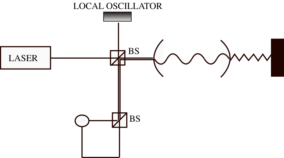
FIG. 1.: Schematical description of the system. The cavity mode is driven by the laser which, thanks to the beam splitter BS, provides also the local oscillator for the homodyne measurement of the light reflected by the cavity.

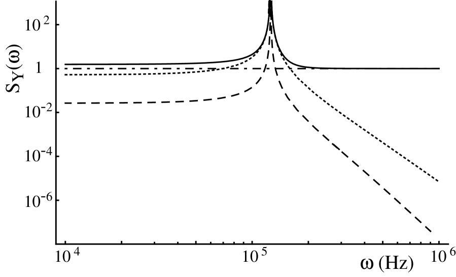
FIG. 2.: Phase noise spectrum of Eq. (61) (full line). The dotted-dashed line refers to the shot noise spectrum (first term of Eq. (61)); the dashed line refers to the radiation pressure term (second term of Eq. (61)), and the dotted line to the thermal noise term (third term of Eq. (61)). Parameter values are $\omega_{\cal S}=1.3\cdot 10^{5}$ Hz, $\eta/m=3\cdot 10^{-2}$ Hz, $\omega_{c}=1.8\cdot 10^{15}$ Hz, $\gamma_{c}=4.7\cdot 10^{5}$ Hz, $m=10^{-5}$ Kg, $L=10^{-2}$ m, $T=4.2$ K, $P=10^{-5}$ W.

REFERENCES

- [1] C.M. Caves, Phys. Rev. Lett. 45, 75 (1980); R. Loudon, Phys. Rev. Lett. 47, 815 (1981); C..M. Caves, Phys. Rev. D 23, 1693 (1981); P. Samphire, R. Loudon and M. Babiker, Phys. Rev. 51, 2726 (1995).
- [2] J. Mertz, O. Marti, and J. Mlynek, Appl. Phys. Lett. 62, 2344 (1993); T.D. Stowe, K. Yasamura, T.W. Kenny, D. Botkin, K. Wago, and D. Rugar, Appl. Phys. Lett. 71, 288 (1997); G.J. Milburn, K. Jacobs, Phys. Rev. A 50, 5256 (1994).
- [3] M. Pinard, C. Fabre, and A. Heidmann, Phys. Rev. A 51, 2443 (1995).
- [4] S. Mancini, V.I. Man’ko, and P. Tombesi, Phys. Rev. A 55, 3042 (1997).
- [5] S. Bose, K. Jacobs, and P.L. Knight, Phys. Rev. A 56, 4175 (1997).
- [6] V.B. Braginsky, Sov. Phys. JETP 26, 831 (1968).
- [7] A. Abramovici et al., Science 256, 325 (1992).
- [8] Y. Hadjar, P.F. Cohadon, C.G. Aminoff, M. Pinard, and A. Heidmann, Europhys. Lett. 47, 545 (1999).
- [9] I. Tittonen, G. Breitenbach, T. Kalkbrenner, T. Müller, R. Conradt, S. Schiller, E. Steinsland, N. Blanc, and N.F. de Rooji, Phys. Rev. A 59, 1038 (1999).
- [10] H. Risken, The Fokker Planck Equation 2nd ed. (Springer, Berlin 1989).
- [11] B. Vacchini, Phys. Rev. Lett. 84, 1374 (2000).
- [12] K. Jacobs, I. Tittonen, H.W. Wiseman and S. Schiller, Phys. Rev. A 60, 538 (1999).
- [13] A.O. Caldeira and A.J. Leggett, Physica A 121, 587 (1983); W.G. Unruh and W.H. Zurek, Phys. Rev. D 40, 1071 (1989).
- [14] L. Diòsi, Europhys. Lett. 22, 1 (1993).
- [15] C. W. Gardiner, Quantum Noise (Springer-Verlag, Berlin, 1991), Chap. 3.
- [16] C. K. Law, Phys. Rev. A 51, 2537 (1995).
- [17] D. F. Walls and G. J. Milburn, Quantum Optics, (Springer, Berlin, 1994).
- [18] G. Lindblad, Commun. Math. Phys. 48, 119 (1976).
- [19] V. Ambegaokar, Ber. Busen-Ges. Phys. Chem. 95, 400 (1991).
- [20] L. Diósi, Physica A 199, 517 (1993).
- [21] S. Gao, Phys. Rev. Lett 79, 3101 (1997).
- [22] F. Haake and R. Reibold, Phys. Rev. A 32, 2462 (1985)
- [23] A.O. Caldeira and A.J. Leggett, Ann. Phys. (N.Y.) 149, 374 (1983).
- [24] G.W. Ford, J.T. Lewis, and R.F. O’Connell, Phys. Rev. A 37, 4419 (1988).
- [25] M.J. Collett, C.W. Gardiner, Phys. Rev. A 30, 1386 (1984); C.W. Gardiner, M.J. Collett, Phys. Rev. A 31, 3761 (1985).
- [26] A. Dorsel, J.D. McCullen, P. Meystre, E. Vignes, and H. Walther, Phys. Rev. Lett. 51, 1550 (1983).
- [27] D. F. Walls and G. J. Milburn, Quantum Optics, (Springer, Berlin, 1994), pag. 124.