The Born Oppenheimer wave function near level crossing

Abstract

The standard Born Oppenheimer theory does not give an accurate description of the wave function near points of level crossing. We give such a description near an isotropic conic crossing, for energies close to the crossing energy. This leads to the study of two coupled second order ordinary differential equations whose solution is described in terms of the generalized hypergeometric functions of the kind ${}_{0}F_{3}(;a,b,c;z)$. We find that, at low angular momenta, the mixing due to crossing is surprisingly large, scaling like $\mu^{1/6}$, where $\mu$ is the electron to nuclear mass ratio.

1 Introduction

In 1927, in a landmark paper, Born and Oppenheimer [2] paved the way to applying quantum mechanics to molecular spectra. In their paper they introduced an approximation that greatly simplified the treatment of quantum mechanical spectral problems in which the particles can be divided into heavy and light. Molecules are an example since the nuclei are much heavier than the electrons. We shall denote by $\mu$ the small parameter of the theory. In molecules $\mu\sim 10^{-4}$, the electron to nucleon mass ratio. Since the light particles are associated with the fast degrees of freedom and the heavy particles with the slow degrees of freedom, the Born Oppenheimer approximation is related to the adiabatic approximation [1, 4, 13]. At the same time, the Born Oppenheimer method can be viewed as a generalized semiclassical approximation where the small parameter $\mu$ plays the role of $\hbar^{2}$. This is a reflection of the fact that the electrons and nuclei also live on different spatial scales, the electronic wave function is spread and is far from the semiclassical limit, while the nuclear wave function is tight and close to semiclassical.

The procedure put forward by Born and Oppenheimer is to first solve the electronic spectral problem with fixed nuclei, and view the nuclear coordinates as parameters. To the leading order in $\mu$, and far from crossings, the heavy degrees of freedom in Born Oppenheimer theory are described by a (scalar) Schrödinger operator in the semiclassical limit with $\hbar^{2}=\mu$ and where the electronic energy surface serves as a potential.

Born Oppenheimer theory developed into two distinct directions. The main direction has been the application to various systems and the development of effective and accurate methods of calculations [8, 9, 10, 11]. The second direction has been the development of the theory as a tool of rigorous spectral theory [3, 4, 5] . Our work falls into the first class.

Points where electronic energy surfaces cross are singular points of the Born Oppenheimer theory. In certain cases, these points can affect spectral properties [8]. In this work we focus on the behaviour of eigenfunctions near crossing. There is surprising little that is known about this. It is not known if the function has finite values at the crossing; how the amplitude of the wave function near the crossing scales with $\mu$. Since crossing controls the mixing of electronic levels, the knowledge of the wave function near crossing is important. Of course, these questions are interesting in the case that the crossing lies in the classically allowed region.

In this work we address these issues for conical (i.e. linear) crossing of two levels where the Born Oppenheimer problem reduces to two coupled Schrödinger equations. In the isotropic case the analysis reduces further to the study of two coupled, second order, ordinary differential equations. We obtain the nuclear wave function analytically, to leading order in $\mu$, close to the crossing. It is related to the generalized hypergeometric functions of the kind ${}_{0}F_{3}$. This function takes the ordinary Born Oppenheimer nuclear wave functions, which are a good approximation far from the crossing, all the way to the crossing, where the nuclear wave function mixes the two electronic levels. We find that the nuclear wave function with total angular momentum $m=\pm\frac{1}{2}$ is nonzero at the crossing point. Moreover, for low momenta, the wave function has a large amplitude near the crossing, of order $\mu^{-1/4}$. We find appreciable mixing of the two levels at distances that are smaller than $\mu^{1/3}$ and the total weight that is mixed between levels scales like $\mu^{1/6}$ which is remarkably large.

2 The Born Oppenheimer approximation

This section is a brief introduction to the basic and elementary elements of Born Oppenheimer theory.

2.1 The basic model

A prototype of the Born Oppenheimer problem, and the one we study here is [8]:

$$H=-\mu\Delta_{x}+H_{e}(x)$$ (1)

where $\mu$ is a small parameter. $H_{e}(x)$ is an operator valued function that acts in the Hilbert space of the light degrees of freedom. Since the eigenvalues of $H_{e}(x)$ repel [15], one does not expect crossing in the case of one heavy coordinate $x$. If $H_{e}(x)$ is time reversal invariant, then stable crossing will occur if there are two heavy coordinates. We therefore assume that $x\in\mathbb{R}^{2}$. For the sake of simplicity we have taken identical masses for the two heavy degrees of freedom. Two degrees of freedom is the simplest case that is still rich enough to cover the phenomena we are interested in.

There are several ways to motivate $H$. The most direct is to think of $H$ as a phenomenological quantization of the molecular vibration. For example, in the case of molecular trimers the two heavy modes are the antisymmetric stretching and bending of the molecule, see fig 1.

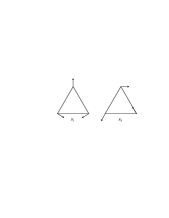
Figure 1: Two degenerate modes in triangular molecules.

Alternatively, one can start with the Schrödinger equation for a molecule, which indeed has the form of Eq. (1) where $H_{e}(x)$ includes the Coulumb potential of the nuclei and the electrons and the electronic kinetic energy. Often, and this is the case in molecules, $H$, is invariant under Gallilean translation and rigid rotation. The symmetry gives three quantum numbers $\{P,J,m\}$ and the spectral analysis of $H_{P,J,m}$ is now restricted to the “internal” nuclear coordinates. In [8] one can find a detailed description of this procedure for a triatomic molecule. $H_{P,J,m}$ has a more complicated expression than $H$: Fixing the center of mass at the origin and restricting to an angular momentum subspace replaces the kinetic energy $-\mu\,\Delta$ by a more general quadratic function of the of the momenta. However, locally near the crossing this expression reduces to [8] Eq. (1).

We shall assume that $H_{e}(x)$ has discrete spectrum and has smooth dependence on the coordinates. In addition, since we shall use the Born Oppenheimer theory as a calculational tool, rather than a tool of spectral analysis, we shall assume that the problem has benign qualitative spectral features. For example, we shall assume that the spectrum of $H$ in the energy range of interest is discrete, and that the associated wave functions are localized in space in the classically allowed region, and that this region is connected. Subtleties associated with tunneling and other exponentially small phenomena will not concern us here.

Since the small parameter $\mu$ multiplies the leading derivative in the $x$ variable, the Born Oppenheimer problem is a version of semiclassical problem where the operator $H_{e}(x)$ replaces the scalar potential $V(x)$.

In molecules there is a second small parameter, $1/c\approx 1/137$, which governs relativistic effects. In particular, spin-orbit interactions, are of order $1/c^{2}$. The lowest order of Born Oppenheimer theory gives an energy scale of $\sqrt{\mu}$ which is comparable to $1/c$ but is much larger than $1/c^{2}$. It is therefore consistent when discussing Born Oppenheimer to leading order to disregard spin-orbit. This is also the reason why we shall not go beyond the leading order.

2.2 Partial Diagonalization

The starting point of the Born Oppenheimer method is to consider $H$ in the basis that diagonalizes the fast (electronic) degrees of freedom.

We assume that the electronic Hamiltonian is real, which is the case in the absence of external magnetic fields. Let $O(x)$ be the orthogonal transformation that diagonalizes $H_{e}(x)$. If $H_{e}(x)$ has simple (non-degenerate) spectrum in the vicinity of $x$ then $O(x)$ is uniquely determined up to multiplication by a diagonal matrix with $\pm 1$ on the diagonal. Locally, one can choose $O(x)$ so that it inherits the smoothness properties of $H_{e}(x)$ [17]. It follows that in the basis that diagonalizes $H_{e}(x)$, Eq. (1) takes the form

$$O^{\dagger}HO=\mu(-i\nabla_{x}-\,A(x))^{2}+E(x),$$ (2)

where $E(x)$ is a diagonal matrix whose entries $E_{j}(x)$ are the electronic energy surfaces and $A(x)=iO^{\dagger}(x)\nabla O(x)$ is a (matrix) gauge field. Since $O(x)$ is real, $A$ is antisymmetric and hermitian. $A$ is responsible to the coupling between electronic energy levels.

One can associate to a crossing point $n$ indices, $\{i_{1},\dots,i_{n}\}$, where $n=dim\ H_{e}$ and $i_{j}=\pm 1$. Let us take a closed curve around a crossing point. After such a cycle $O(x)$ must return to itself up to up to multiplication by a diagonal matrix with entries $\pm 1$ on the diagonal. These entries are the indices of the crossing. It is known [7] that for a conic crossing between the $j-th$ and $j+1$ eigenvalues of $H_{e}(x)$ give $i_{j}=i_{j+1}=-1$ and all other indices are, of course, $+1$.

For conic (linear) crossing $O(x)$ flips signs on a circle of radius $|x|$ [7]. Therefore its gradient must be of order $1/|x|$. This makes $A$ of order $1/|x|$. It follows that the coupling between electronic states diverges like a simple pole near crossing.

This completes the local description of the theory. The problem also has an interesting global aspect. Since $H_{e}(x)$ is a real symmetric matrix, the Wigner von Neumann crossing rule [15] says that $H_{e}(x),\ x\in\mathbb{R}^{2}$ has, generically, isolated crossing points. As a consequence, with points of crossing being removed the plane becomes multiply connected (see fig. 2)

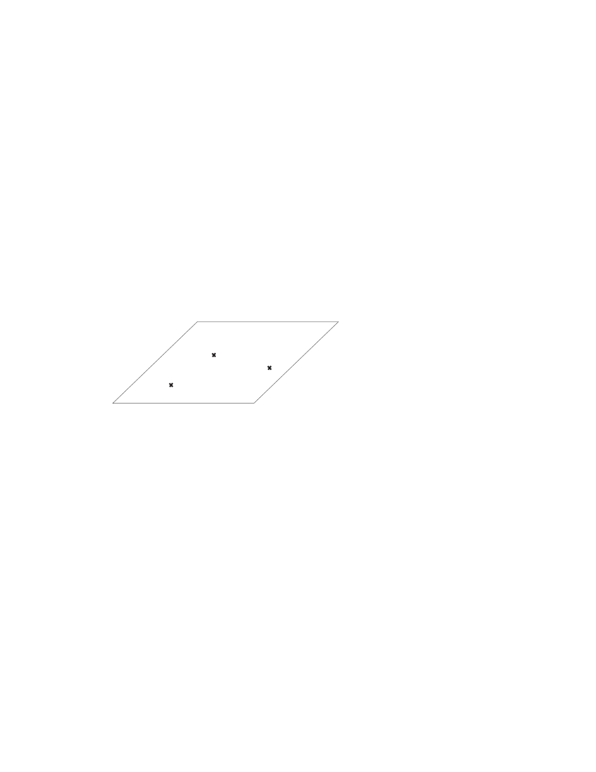
Figure 2: With points of crossing removed the plane becomes multiply connected.

We can now describe the boundary conditions associated with Eq. (2). The general case of several crossing points can be complicated but in the case of at most one point of crossing the situation is simple. In that case, cut the plane from the crossing point to infinity. On the cut plane $O(x)$ is uniquely defined in a continuous way. Then the boundary condition on the j-th component of the wave function associated with Eq. (2) is periodic or anti-periodic according to the index $i_{j}$.

2.2.1 Born Oppenheimer theory near a non-degenerate minimum

Let $x=0$ be a minimizer of an electronic energy surface. Pick the origin so that the minimum is at zero energy (see Fig. 3).

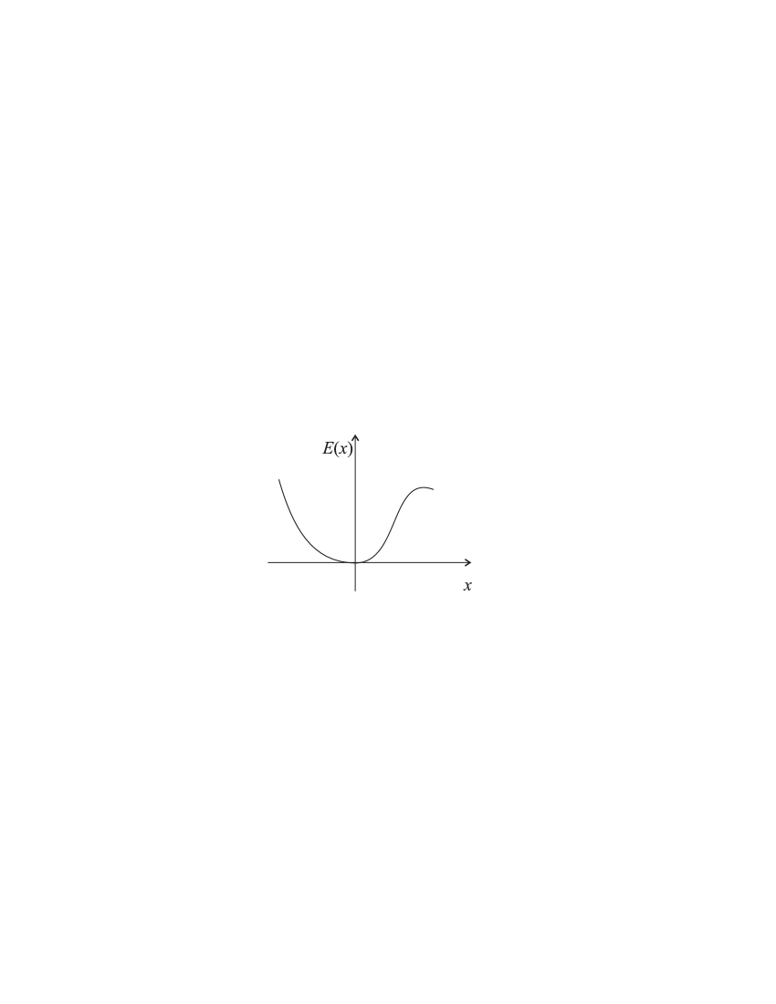
Figure 3: A potential energy surface near a non-degenerate minimum.

Upon scaling, $x=\mu^{1/4}\xi$, the Born Oppenheimer operator assumes the form

$$\sqrt{\mu}\left((-i\nabla_{\xi}-\varepsilon\,A(\varepsilon\xi))^{2}+\,\frac{1}{\sqrt{\mu}}\,E(\varepsilon\xi)\right),\quad\varepsilon=\mu^{1/4}.$$ (3)

The (scaled, matrix) potential energy is $O(1)$ for the electronic energy surface near the minimum, and has gaps of order $\mu^{-1/2}$ to (scaled) “excited electronic states”. Suppose first that there is no crossing. Then the coupling between electronic levels is small, $\varepsilon\,A(\varepsilon\xi)=O(\mu^{1/4})$, and a perturbation argument shows that the effect on eigenvalues is of order $O(\mu)$ (in unscaled energy) and of order $O(\mu^{3/4})$ for the wave function. It follows that the spectral analysis in an energy interval of order $o(1)$ near the minimum, reduces to an ordinary Schrödinger equation (not matrix valued) with no vector potential (since $A$ vanishes on the diagonal). This accounts for $o(1/\mu)$ eigenvalues near the minimum in two dimensions.

Now, if there is a point of crossing, there are two possibilities. The first, and simplest, is that the crossing lies in the classically forbidden region, see Fig 4.

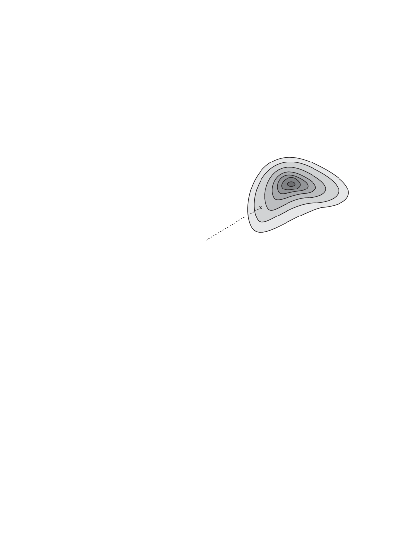
Figure 4: For a non-degenerate minimum, when the crossing falls in a classically forbidden region, the cut to infinity can be pushed to the classically forbidden zone, and one can forget about the crosing to leading order.

Then the divergent vector potential is harmless, since the wave function is $\exp(-\frac{1}{\sqrt{\mu}})$ near the crossing. The cut to infinity can be pushed to the classically forbidden zone, so the difference between periodic or anti-periodic boundary conditions is exponentially small, and one can forget about the crossing altogether. If the crossing point lies in the classically allowed region, it couples two nuclear Scrödinger equations and ruins the traditional Born Oppenheimer approximation.

2.2.2 Born Oppenheimer theory near a degenerate minimizer

It can happen that the crossing must be taken into account although it lies at the classically forbidden zone. This happens when the cut can not be pushed to the classically forbidden zone. This is the case, for example, when the curve $\gamma\in\mathbb{R}^{2}$ is a minimizer of an electronic energy surface with zero energy on $\gamma$. If $\gamma$ encircles a crossing (see Fig. 5)

Figure 5: A degenerate minimum around a crossing. The solid circle represents $\gamma$. Although the crossing falls in the classically forbidden zone, it should be taken into account.

then the cut necessarily intersects $\gamma$ and since $\gamma$ lies in the classically accessible region, the wave function is large there and it matters if one imposes periodic or anti-periodic boundary conditions.

3 Born Oppenheimer theory near crossing

Consider now the spectral problem near crossing energy of two electronic energy surfaces. Let us set the crossing energy at $0$ and assume that the crossing is conic. This is the generic situation.

Upon scaling, $x=\epsilon\xi,\ \epsilon=\mu^{1/3}$, the Born Oppenheimer operator assumes the form

$$\epsilon\left((-i\nabla_{\xi}-\epsilon\,A(\epsilon\xi))^{2}+\,\frac{1}{\epsilon}\,E(\epsilon\xi)\right),\quad\epsilon=\mu^{1/3}.$$ (4)

The scaling increases the gaps between the electronic energy surfaces and decreases the coupling of the crossing pair to other levels since $\epsilon\,A_{ij}(\epsilon\xi)=O(\mu^{1/3})$ when $i$ belongs to the pair and $j$ to other levels. On the other hand, the crossing pair remains coupled, because the Coulombic singularity near the crossing says that $\epsilon A_{i,i^{\prime}}(\epsilon\xi)=O\left(\frac{1}{|\xi|}\right)$, which is large when $\xi$ is small. We see that a spectral problem in an interval of order $o(1)$ near the crossing energy, reduces to a problem where $H_{e}(x)$ is a $2\times 2$ matrix up to an error of order $\mu$ in the eigenvalues and of order $\mu^{2/3}$ in the eigenfunctions.

Our aim, in this work, is to describe the wave functions for states, located at an interval of width that is much smaller than $\mu^{1/3}$ near the crossing. Even though this is a small interval, it has lots of eigenvalues: By Weyl’s rule there are many states, of order $\mu^{-2/3}$, in an interval of width $\mu^{1/3}$, in two dimensions. One can expect to find many states in the interval in question.

Close to the crossing $H_{e}(x)$ can be expanded in terms of the Pauli matrices and the unit matrix. We assume that asymptotically close to the crossing point $H_{e}(x)$ is isotropic and conic:

$$H_{e}(x)=\sigma\cdot x+O(x^{2}).$$ (5)

We choose $\sigma_{1,2}$ real:

$$\sigma_{1}=\pmatrix{0&1\cr 1&0},\quad\sigma_{2}=\pmatrix{1&0\cr 0&-1}.$$ (6)

$O(x^{2})$ accounts for the behaviour far from the crossing which is not universal, or isotropic.

How restrictive is the assumption that near the crossing $H_{e}(x)$ is isotropic? Molecules are never isotropic, although some may be approximately so. Nevertheless, isotropic conic intersections are, in fact, common. This is a known phenomenon in group theory: Discrete symmetry can force full continuous symmetry on tensors of finite rank [22]. For example, as shown by [9], the $D_{3}$ symmetry of trimers forces isotropy of the conics.

It follows from the above that if one is interested in the local behavior of eigenfunctions for eigenvalues that lie in an energy range that is small compared to $\mu^{1/3}$ and in a spatial neighborhood of the crossing, $|x|<<1$, the eigenfunctions satisfy, to leading order in $\mu$, a canonical system of partial differential equations,

$$\Big{(}-\mu\,\Delta_{xx}+\sigma\cdot x\Big{)}\Psi=\mu^{1/3}\Big{(}-\,\Delta_{\xi\xi}+\sigma\cdot\xi\Big{)}\Psi=0.$$ (7)

The rotational symmetry allows us to reduce the system Eq. (7), to a system of linear, ordinary differential equation parameterized by angular momentum $m\in\mathbb{Z}+\frac{1}{2}$ (see section 4.1):

$$\left\{-\frac{d^{2}}{d\rho^{2}}-\frac{1}{\rho}\frac{d}{d\rho}+\frac{m^{2}+1/4}{\rho^{2}}+\pmatrix{-\frac{m}{\rho^{2}}&\rho\cr\rho&\frac{m}{\rho^{2}}}\right\}{\cal F}_{m}=0,\quad\rho=|\xi|.$$ (8)

For fixed $m$ the space of solutions of the ODE is four dimensional. We shall see that there is a one dimensional subspace of solutions that is well behaved near the origin $\rho=0$, and near infinity. As we shall explain, functions in this space describe the asymptotic behavior of eigenfunctions with energies near the crossing and spatially close to it. The explicit expression for these solutions, is described below.

3.1 The main result

We now describe our main result:

Theorem 3.1

For $m\in\mathbb{Z}+\frac{1}{2}$, and $m\geq\frac{1}{2}$, let

$${\cal F}_{m}(\rho) = \frac{3^{-\frac{1}{2}}6^{-(\frac{5}{6}+\frac{2m}{3})}\rho^{m-\frac{1}{2}}}{\Gamma(\frac{2}{3})\Gamma(\frac{1}{2}+\frac{m}{3})\,\Gamma(\frac{7}{6}+\frac{m}{3})\,}\,\pmatrix{{{}_{0}F_{3}}(;\frac{1}{3},\frac{1}{2}+\frac{m}{3},\frac{5}{6}+\frac{m}{3};\frac{\rho^{6}}{6^{4}})\cr\frac{\rho^{3}}{6+4m}{{}_{0}F_{3}}(;\frac{4}{3},\frac{3}{2}+\frac{m}{3},\frac{5}{6}+\frac{m}{3};\frac{\rho^{6}}{6^{4}})}$$

$$- \frac{3^{-\frac{1}{2}}\,\,6^{-(\frac{1}{6}+\frac{2m}{3})}\,\rho^{m+\frac{1}{2}}}{{\Gamma(\frac{1}{3})\Gamma(\frac{1}{2}+\frac{m}{3})\Gamma(\frac{5}{6}+\frac{m}{3})}}\,\pmatrix{\frac{\rho^{3}}{12+8m}{{}_{0}F_{3}}(;\frac{5}{3},\frac{3}{2}+\frac{m}{3},\frac{7}{6}+\frac{m}{3};\frac{\rho^{6}}{6^{4}})\cr{{}_{0}F_{3}}(;\frac{2}{3},\frac{1}{2}+\frac{m}{3},\frac{7}{6}+\frac{m}{3};\frac{\rho^{6}}{6^{4}})}$$

then

• ${\cal F}_{m}(\rho)$, is a solution of the system of differential equations, Eq. (8).

• For small $\rho$

  $${\cal F}_{m}(\rho)\to\frac{\,3^{-\frac{1}{2}}\rho^{m-\frac{1}{2}}}{\Gamma(\frac{1}{2}+\frac{m}{3})6^{\frac{4m+1}{6}}}\pmatrix{\frac{1}{\Gamma(\frac{2}{3})\Gamma(\frac{7}{6}+\frac{m}{3})6^{\frac{2}{3}}}\cr-\frac{\rho}{\Gamma(\frac{1}{3})\Gamma(\frac{5}{6}+\frac{m}{3})}}.$$ (12)

  In particular, ${\cal F}_{\frac{1}{2}}(0)\neq 0.$

• For large $\rho$

  $${\cal F}_{m}(\rho)\to\frac{1}{(2\pi)^{3/2}\rho^{3/4}}\cos\left(\frac{2}{3}\rho^{3/2}-\pi\left(\frac{m}{3}+\frac{1}{4}\right)\right)\pmatrix{1\cr-1}$$ (13)

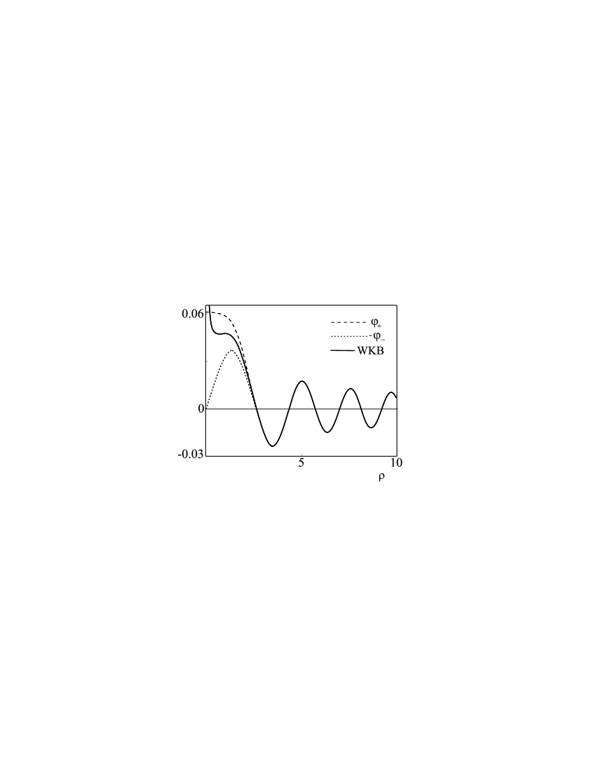
Figure 6: The components of ${\cal F}_{m}(\rho)$ for $m=\frac{1}{2}$ and their asymptotic form given by (13). The function is compared with the WKB Born Oppenheimer wave function.

Theorem 3.2

For $m\in\mathbb{Z}+\frac{1}{2}$, and $m\geq\frac{1}{2}$, let

$$\Psi_{m}(r,\theta)=\mu^{-1/4}e^{im\theta}\,\pmatrix{e^{i\theta/2}&ie^{-i\theta/2}\cr ie^{i\theta/2}&e^{-i\theta/2}}\,{\cal F}_{m}(\mu^{-1/3}r)$$ (14)

then

• $\Psi_{m}$ is a solution of the system of PDE, Eq. (7) where $x=(r\cos\theta,r\sin\theta)$.

• The m-th component of an eigenfunction of Eq. (1) near crossing, i.e. with eigenvalue $|E|<<\mu^{1/3}$ and for $x=(r\cos\theta,r\sin\theta),\ r<<1$ is, to leading order, proportional to $\Psi_{m}(r,\theta)$.

• The amplitude of $\Psi_{m}$ is independent of $\mu$ in the region $r>>\mu^{1/3}$.

• Near the crossing, $r\approx\mu^{1/3}$, the amplitude of the wave function $\Psi_{m}=O(\mu^{-1/4})$

Remark 3.1

The most interesting aspect of the solution is that the wave function has large amplitude at the crossing region in the limit of small $\mu$. As we shall see, this result follows from arguments that do not rely on the explicit form of the solution, but do depend on the fact that in the non-mixing region, $r>>\mu^{1/3}$ the solution has a WKB form in the radial direction.

Remark 3.2

The function $\Psi_{m}$ does not describe the behavior of wave functions in the far zone where $r>1$. The behaviour in the far zone is not universal and depends on the details of the electronic energy surface . The far zone is described by standard Born Oppenheimer, so $\Psi_{m}$ gives complementary information.

Remark 3.3

There are $o\left(\mu^{-2/3}\right)$ states in the relevant energy interval $o\left(\mu^{1/3}\right)$ near the crossing disregarding $m$. For a given $m$ there are only $\mu^{-1/6}$ levels in this interval. This says that near the crossing $m$ is bounded by order $\mu^{-1/2}$.

Remark 3.4

We shall actually only prove the theorem in the special case that $H_{e}(x)$ is rotationally symmetric. The symmetry decouples channels with different angular momenta. We believe that mixing of angular momenta in the far zone is only a technical complication and that the result also holds without rotational symmetry in the far zone.

4 The Rotationally Symmetric Case

In the following we describe a derivation of the main result for a Born Oppenheimer model that is rotationally symmetric. With rotational symmetry we can reduce the spectral problem of a PDE to a spectral problem of an ODE. No real molecule is rotationally symmetric and the general case leads to mixing of $m$ channels. We believe that this is only a technical complication.

We require invariance of $H_{e}(x)$ under infinitesimal rotations in the nuclear and electronic Hilbert spaces. Such a rotation is generated by

$$J_{3}=L_{3}+\frac{1}{2}\sigma_{3}=-ix_{1}\frac{\partial}{\partial x_{2}}+ix_{2}\frac{\partial}{\partial x_{1}}+\frac{1}{2}\sigma_{3},$$ (15)

with

$$\sigma_{3}=\pmatrix{0&i\cr-i&0}.$$

The $L_{3}$ part generates $SO(2)$ rotations in the nuclear Hilbert space ($x_{1}-x_{2}$ plane), whereas the $\frac{1}{2}\sigma_{3}$ part generates a rotation in the electronic Hilbert space. $J_{3}$ does not have the meaning of total angular momentum since the Pauli matrices do not represent spin. Isotropy means that $J_{3}$ commutes with $H_{e}(x)$:

$$0=[J_{3},H_{e}(x)]$$

The most general form of $H_{e}(x)$ for a two level system that is rotationally symmetric and real is:

$$H_{e}(x)=Q_{0}(r)+Q_{1}(r)(x\cdot\sigma)+Q_{2}(r)(x\times\sigma),\quad r=|x|$$ (16)

An additional $Q_{3}(r)\sigma_{3}$ term in (16) is allowed by rotational invariance but it is forbidden by time reversal symmetry, since $\sigma_{3}$ is imaginary.

The energy surfaces of $H_{e}(x)$ are equal to

$$E_{\pm}(r)=Q_{0}(r)\pm q(r);\quad q(r)=r\sqrt{Q_{1}^{2}(r)+Q_{2}^{2}(r)}$$ (17)

We shall assume that $Q_{0,1,2}$ are smooth functions of $r$ and that $Q_{1}(0)=1$ while $Q_{0,2}(r)=O(r^{2})$ for small $r$. This gives conic intersection at zero with $E_{\pm}(r)=\pm r$, see Fig. 7.

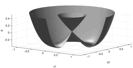
Figure 7: The electronic energy surfaces of $H_{e}(x)$

4.1 The radial Hamiltonian

The spectral subspace of $J_{3}$, with eigenvalue $m$ is spanned by

$$e_{1}=e^{i(m+1/2)\theta}\pmatrix{1\cr i}\,\quad e_{2}=e^{i(m-1/2)\theta}\pmatrix{i\cr 1}$$ (18)

$m$ must be half odd integer for $e_{1,2}$ to be univalued, i.e. $m\in\mathbb{Z}+\frac{1}{2}$.

Since

$$-\Delta\,e_{1}=\frac{(m+\frac{1}{2})^{2}}{r^{2}}\,e_{1}, \quad-\Delta\,e_{2}=\frac{(m-\frac{1}{2})^{2}}{r^{2}}\,e_{2},$$ (19)

$$x\cdot\sigma\,e_{1}=r\,e_{2}, \quad x\cdot\sigma\,e_{2}=r\,e_{1},$$ (20)

$$x\times\sigma\,e_{1}=-ir\,e_{2}, \quad x\times\sigma\,e_{2}=ir\,e_{1},$$ (21)

in terms of the basis $\{e_{1},e_{2}\}$ we obtain for the radial equation:

$$H(m,\mu)=-\mu\left(\frac{d^{2}}{dr^{2}}+\frac{1}{r}\frac{d}{dr}-\frac{1}{4r^{2}}\right)+H_{e}(r,\mu,m)$$ (22)

with

$$H_{e}(r,\mu,m)=Q_{0}(r)+rQ_{1}(r)\sigma_{1}+rQ_{2}(r)\sigma_{3}-\frac{\mu}{r^{2}}\left({m}\sigma_{2}-m^{2}\right)$$ (23)

Scaling $r=\mu^{1/3}\rho$ we get Eq. (8), to leading order in $\mu$, for $0\leq\rho<<\mu^{-1/3}$.

Remark 4.1

The radial Hamiltonian, $H_{e}(m,\mu,r)$, actually has no level crossing. This, by itself, does not ameliorate the mixing of the two levels for now the gap in the spectrum of $H_{e}(m,\mu,r)$ is of order $\mu^{1/3}$. The smallness of this gap leads to mixing of the electronic levels.

We shall restrict ourselves to $m>0$. Since

$$\sigma_{1}\,H^{*}_{e}(r,\mu,m)\sigma_{1}=H_{e}(r,\mu,-m),$$ (24)

$H(m,\mu)$ and $H(-m,\mu)$ are isospectral and the radial part of the function with $-m$ can be obtained from the one with $+m$ by interchanging upper and lower components and taking complex conjugates.

4.2 The Indicial equation

The origin, $\rho=0$ is regular-singular point [20] of the equation. Substituting

$$\pmatrix{\rho^{\alpha}\cr\rho^{\beta}}(1+O(\rho))$$ (25)

into (8) we obtain the roots ${\alpha}=\pm(m-\frac{1}{2})$ and ${\beta}=\pm(m+\frac{1}{2})$. Equation (8) therefore has four linearly independent solutions, which asymptotically near the origin, behave like

$$\pmatrix{\rho^{m-\frac{1}{2}}\cr 0};\,\,\pmatrix{\rho^{-m+\frac{1}{2}}\cr 0};\,\,\pmatrix{0\cr\rho^{m+\frac{1}{2}}};\,\,\pmatrix{0\cr\rho^{-m-\frac{1}{2}}}$$ (26)

(26) is correct only for $|m|\neq\frac{1}{2}$. The case $|m|=\frac{1}{2}$ requires special treatment, because of the two degenerate roots in the upper component. For $|m|=\frac{1}{2}$ the four linearly independent solutions behave asymptotically near the origin like [20]

$$\pmatrix{1\cr 0};\quad\pmatrix{\ln(\rho)\cr 0};\quad\pmatrix{0\cr\rho};\quad\pmatrix{0\cr 1/\rho}$$ (27)

We see that for any $m$ there are always two solutions which are bounded near the origin and two others which are divergent. Since a smooth Hamiltonian can give rise to smooth eigenfunctions only [21] in the four dimensional space of solutions to the differential equation, there is a two dimensional subspace of admissible solutions, the ones which are well behaved at the origin.

4.3 Solution to the ODE

In this section we show that the solutions of Eq. (8) that are regular at the origin, can be explicitly constructed in terms of certain Hypergeometric functions.

Theorem 4.1

The solutions of (8) which are bounded at the origin are spanned by:

$${\cal F}_{m}^{(1)}(\rho) = \pmatrix{\varphi_{+}^{(1)}(\rho)\cr\varphi_{-}^{(1)}(\rho)}=\pmatrix{\rho^{m-\frac{1}{2}}{{}_{0}F_{3}}(;\frac{1}{3},\frac{1}{2}+\frac{m}{3},\frac{5}{6}+\frac{m}{3};\frac{\rho^{6}}{6^{4}})\cr\frac{\rho^{m+\frac{5}{2}}}{6+4m}{{}_{0}F_{3}}(;\frac{4}{3},\frac{3}{2}+\frac{m}{3},\frac{5}{6}+\frac{m}{3};\frac{\rho^{6}}{6^{4}})};$$ (28)

$${\cal F}_{m}^{(2)}(\rho) = \pmatrix{\varphi_{+}^{(2)}(\rho)\cr\varphi_{-}^{(2)}(\rho)}=\pmatrix{\frac{\rho^{m+\frac{7}{2}}}{12+8m}{{}_{0}F_{3}}(;\frac{5}{3},\frac{3}{2}+\frac{m}{3},\frac{7}{6}+\frac{m}{3};\frac{\rho^{6}}{6^{4}})\cr\rho^{m+\frac{1}{2}}{{}_{0}F_{3}}(;\frac{2}{3},\frac{1}{2}+\frac{m}{3},\frac{7}{6}+\frac{m}{3};\frac{\rho^{6}}{6^{4}})},\phantom{==}$$ (30)

where ${}_{0}F_{3}(;a,b,c;x)$ are the generalized hypergeometric functions of the kind ${}_{0}F_{3}$.

Proof: Under scaling, $\rho\to\lambda\rho$, Eq. (8) transforms to

$$\left\{-\frac{d^{2}}{d\rho^{2}}-\frac{1}{\rho}\frac{d}{d\rho}+\frac{m^{2}+1/4}{\rho^{2}}+\pmatrix{-\frac{m}{\rho^{2}}&\lambda^{3}\rho\cr\lambda^{3}\rho&\frac{m}{\rho^{2}}}\right\}{\cal F}_{m}(\lambda\rho)=0.$$ (31)

In particular, the equation is invariant under scaling by $\lambda$, a cube root of unity, $\lambda=e^{2\pi i/3}$. (Note that this feature is lost when one considers solutions of the equation for non-zero eigenvalue.) By an analog of Bloch theorem, the solution is a product of an eigenfunction of the scaling transformation and a periodic function under scaling by $e^{2\pi i/3}$. $\rho^{\alpha}$ is an eigenfunction of the scaling transformation with eigenvalue $\lambda^{\alpha}$. Hence that ${\cal F}_{m}$ must be of the form $\rho^{\alpha}\,{\cal G}(\rho^{3})$. The indicial equation fixes $\alpha=m-1/2$. ${\cal G}_{m}(\rho^{3})$ is then an analytic function of its argument.

The space of solutions regular of this kind is two dimensional and gives a representation of $D_{3}$, the group of discrete rotations by $2\pi/3$. Since the only complex irreducible representations [19] of $D_{3}$ are the complex numbers $\omega$, such that $\omega^{3}=1$, one can always find a basis ${\cal F}_{m}^{(1)}(\rho),{\cal F}_{m}^{(2)}(\rho)$ such that

$${\cal F}_{m}^{(j)}(e^{2\pi i/3}\rho)=\omega_{j}{\cal F}_{m}^{(j)}(\rho).$$

This condition fixes the solutions in Eq. (28) where $\omega_{1}=e^{2\pi i(m-1/2)/3}$ and $\omega_{2}=e^{2\pi i(m+1/2)/3}$.

To relate ${\cal G}_{m}$ to hypergeometric functions we turn the two coupled second order equations (8) into a scalar fourth order equation for each component. The equations obtained for the component $\varphi_{+}$ and $\varphi_{-}$ can be written, with $\zeta=\rho^{6}/6^{4}$, and ${\rm D}=\zeta\frac{d}{d\zeta}$, in the form:

$$\left\{{\rm D}\left({\rm D}-\frac{2}{3}\right)\left({\rm D}+\frac{m}{3}-\frac{1}{2}\right)\left({\rm D}+\frac{m}{3}-\frac{1}{6}\right)-\zeta\right\}\zeta^{\frac{-m+1/2}{6}}\varphi_{+}(\zeta)=0$$ (32)

$$\left\{{\rm D}\left({\rm D}-\frac{1}{3}\right)\left({\rm D}+\frac{m}{3}-\frac{1}{2}\right)\left({\rm D}+\frac{m}{3}+\frac{1}{6}\right)-\zeta\right\}\zeta^{\frac{-m-1/2}{6}}\varphi_{-}(\zeta)=0$$ (33)

The generalized hypergeometric function ${}_{0}F_{3}(;a,b,c;\zeta)$ is defined by [24]:

$${{}_{0}F_{3}}(;a,b,c;\zeta)=\sum_{k=0}^{\infty}\frac{\Gamma(a)\Gamma(b)\Gamma(c)}{k!\Gamma(k+a)\Gamma(k+b)\Gamma(k+c)}\zeta^{k}.$$ (34)

It is a matter of calculation to see that it satisfies the differential equation:

$$\left\{{\rm D}({\rm D}+a-1)({\rm D}+b-1)({\rm D}+c-1)-\zeta\right\}{{}_{0}F_{3}}(;a,b,c;\zeta)=0.$$ (35)

Eq. (32) is a special case of this. Note, however, that we are not free to pick both $\varphi_{+}^{(1)}$ and $\varphi_{-}^{(1)}$ as the hypergeometric functions corresponding to Eq. (35). We can pick one, and then the other is determined by Eq. (8).

To get ${\cal F}^{(1)}_{m}$ we pick the upper component to be the hypergeometric function that solves Eq. (32), i.e.

$$\varphi_{+}^{(1)}(\rho)=\rho^{m-\frac{1}{2}}{{}_{0}F_{3}}\left(;\frac{1}{3},\frac{1}{2}+\frac{m}{3},\frac{5}{6}+\frac{m}{3};\frac{\rho^{6}}{6^{4}}\right).$$

The lower component,$\varphi_{-}^{(1)}$, is determined by (8), which gives us the relation

$$\varphi_{-}^{(1)}(\rho)=\frac{\rho^{m-\frac{1}{2}}}{\rho^{3}}\left\{\rho\frac{d}{d\rho}\left(\rho\frac{d}{d\rho}+2m-1\right)\right\}\frac{\varphi_{+}^{(1)}(\rho)}{\rho^{m-\frac{1}{2}}}$$ (36)

With the identities [24, 26]

$$\left(\zeta\frac{d}{d\zeta}+c-1\right){{}_{0}F_{3}}(;a,b,c;\zeta) = (c-1){{}_{0}F_{3}}(;a,b,c-1;\zeta)$$ (37)

$$\frac{d}{d\zeta}{{}_{0}F_{3}}(;a,b,c;\zeta) = \frac{1}{abc}{{}_{0}F_{3}}(;a+1,b+1,c+1;\zeta)$$

we obtain

$$\varphi_{-}^{(1)}(\rho)=\frac{1}{6+4m}\rho^{m+\frac{5}{2}}{{}_{0}F_{3}}\left(;\frac{4}{3},\frac{3}{2}+\frac{m}{3},\frac{5}{6}+\frac{m}{3};\frac{\rho^{6}}{6^{4}}\right).$$ (38)

The second solution, ${\cal F}^{(2)}_{m}$, is obtained by picking $\varphi_{-}^{(2)}$ to be the hypergeometric solution to Eq. (32). Namely,

$$\varphi_{-}^{(2)}(\rho)=\rho^{m+\frac{1}{2}}{{}_{0}F_{3}}\left(;\frac{2}{3},\frac{1}{2}+\frac{m}{3},\frac{7}{6}+\frac{m}{3};\frac{\rho^{6}}{6^{4}}\right).$$ (39)

and with a relation

$$\varphi_{+}^{(2)}(\rho)=\frac{\rho^{m+\frac{1}{2}}}{\rho^{3}}\left\{\rho\frac{d}{d\rho}\left(\rho\frac{d}{d\rho}+2m+1\right)\right\}\frac{\varphi_{-}^{(2)}(m;\rho)}{\rho^{m+\frac{1}{2}}}$$

similar to (36) one computes the upper component of the second solution:

$$\varphi_{+}^{(2)}(\rho)=\frac{1}{12+8m}\rho^{m+\frac{7}{2}}{{}_{0}F_{3}}\left(;\frac{5}{3},\frac{3}{2}+\frac{m}{3},\frac{7}{6}+\frac{m}{3};\frac{\rho^{6}}{6^{4}}\right)\hfill\blacksquare$$

4.4 The well behaved solutions

We have seen that of the four dimensional family of solution of Eq.(8) there is a distinguished two dimensional family that is well behaved near the origin. We shall now show that there is a three dimensional family that is well behaved at infinity:

Theorem 4.2

• In the four dimensional space of solutions of Eq. (8) there is a three dimensional family of solutions that vanish at infinity, and one dimensional subspace that diverges exponentially at infinity.

• The solutions of (8) for $\rho>>1$ are (asymptotically) spanned by the four dimensional family :

  $$\rho^{-3/4}\,\exp\left({-\frac{2}{3}\rho^{3/2}}\right)\,\pmatrix{1\cr 1}; \quad\rho^{-3/4}\,\exp\left({\frac{2}{3}\rho^{3/2}}\right)\,\pmatrix{1\cr 1};$$

  $$\rho^{-3/4}\,\cos\left(\frac{2}{3}\rho^{3/2}\right)\,\pmatrix{1\cr-1}; \quad\rho^{-3/4}\,\sin\left(\frac{2}{3}\rho^{3/2}\right)\,\pmatrix{1\cr-1}.$$ (40)

• The exponential blow up of ${\cal F}_{m}^{(1,2)}$ of Eq. (8) is given by

  $$2{\cal F}_{m}^{(1)}(\rho) \to {\Gamma\left(\frac{1}{3}\right)\Gamma\left(\frac{1}{2}+\frac{m}{3}\right)\Gamma\left(\frac{5}{6}+\frac{m}{3}\right)6^{\frac{1}{6}+\frac{2m}{3}}}\rho^{-3/4}\,\exp\left({\frac{2}{3}\rho^{3/2}}\right)\,\pmatrix{1\cr 1}$$

  $$2{\cal F}_{m}^{(2)}(\rho) \to {\Gamma\left(\frac{2}{3}\right)\Gamma\left(\frac{1}{2}+\frac{m}{3}\right)\Gamma\left(\frac{7}{6}+\frac{m}{3}\right)6^{\frac{5}{6}+\frac{2m}{3}}}\rho^{-3/4}\,\exp\left({\frac{2}{3}\rho^{3/2}}\right)\,\pmatrix{1\cr 1}$$

• The solution to Eq (8) that vanishes at the origin and at infinity is a multiple of

  $${\Gamma\left(\frac{2}{3}\right)\Gamma\left(\frac{1}{2}+\frac{m}{3}\right)\Gamma\left(\frac{7}{6}+\frac{m}{3}\right)6^{\frac{5}{6}}}\,{\cal F}_{m}^{(1)}(\rho)-$$

  $${\Gamma\left(\frac{1}{3}\right)\Gamma\left(\frac{1}{2}+\frac{m}{3}\right)\Gamma\left(\frac{5}{6}+\frac{m}{3}\right)6^{\frac{1}{6}}}\,{\cal F}_{m}^{(2)}(\rho).$$

Proof: $H_{e}(\rho,\mu,m)$ for Eq. (8) is, for $\rho>>1$,

$$H_{e}(\rho,\mu,m)=\frac{m^{2}+1/4}{\rho^{2}}+\pmatrix{-\frac{m}{\rho^{2}}&\rho\cr\rho&\frac{m}{\rho^{2}}}\approx\pmatrix{0&\rho\cr\rho&0}$$ (41)

With eigenvalues $\pm\rho$. It follows that the solution for large $\rho$ reduces to the study of two uncoupeld equations:

$$\left(-\frac{d^{2}}{d\rho^{2}}-\frac{1}{\rho}\frac{d}{d\rho}\pm\rho\right)\psi=0.$$ (42)

Since $\rho$ is large, these can be solved by WKB to give the first part of the theorem. The blow up of the solutions at infinity can be obtained from the relation (omitting the exponentially decaying part)

$$_{0}F_{3}(;a,b,c;x)\to\frac{\Gamma(a)\Gamma(b)\Gamma(c)}{2(2\pi)^{3/2}}x^{\gamma}\left(e^{4x^{\frac{1}{4}}}+2\cos(4x^{\frac{1}{4}}+2\pi\gamma)\right),$$ (43)

with $\gamma=-\frac{a+b+c-3/2}{4}$. This relation can be obtained by studying the asymptotic behavior of the coefficients in the series of ${}_{0}F_{3}$. Alternatively, in [23], the asymptotic form of the generalized hypergeometric functions ${}_{p}F_{q}$ is derived, and the formula given there reduces to (43) after substituting $q=0,p=3$, computing the summations and omitting the exponentially decaying part.

¿From this the rest follows, as well as the proof of theorem 3.1. $\blacksquare$

It remains to explain how eigenvectors are related to these well behaved solutions. The point is that the canonical differential equation approximates the eigenvalue equation only for $r<<1$, or, equivalently, for $\rho<<\mu^{-1/3}$. Consider an eigenfunction. Far from the crossing this eigenfunction can be approximated by a WKB solution, and it is clear that this WKB solution can be approximated by WKB solution of the canonical problem in the interval $\mu^{-1/3}>>\rho>>1$. The component that blows up must have an exponentially small amplitude, of order $\exp(-\frac{2}{3\sqrt{\mu}})$, and, to leading order can be neglected near the crossing.

5 Anomalous Mixing

The basic and fundamental observation of the Born Oppenheimer theory is the emergence of the energy scale $\sqrt{\mu}$ in molecular spectra associated with vibrations. Perhaps the most interesting observation that results from the analysis of the Born Oppenheimer theory near crossing, is that emergence of the scale, $\mu^{1/6}$, associated with mixing at crossing. $\mu^{1/6}$ is normally not a small number: In molecules $\mu^{1/6}\sim.2$.

Classically, a uniform density on the energy shell, $\delta(p^{2}+V(x)-E)$ implies that, in two dimensions, the spatial density is also uniform on the classically allowed region. The region where there is substantial mixing between the two electronic energy surfaces has linear dimensions that scale like $\mu^{1/3}$. For a crossing point in two dimension the volume characterizing the mixing therefore scales like $\mu^{2/3}$. The semiclassical expectation is therefore that mixing near crossing should scale like the area $\mu^{2/3}$.

For isotropic crossing we found that the wave function has anomalously large amplitude in the mixing region for values of azymuthal quantum numbers that are small compares to $\mu^{-1/2}$. For these, from theorem 3.2, the amplitude in the near zone scales like $\mu^{-1/4}$. This implies that the total mixing weight scales like $\mu^{1/6}$.

It would be interesting to have a more complete picture of the mixing near non-isotropic crossing and also for chaotic systems.

References

- [1] J.E. Avron and A. Elgart, Comm. Math. Phys., 203, 445-463, (1999)
- [2] M. Born and R. Oppenheimer, Ann. Phys. (Leipzig) 84, 457 (1927)
- [3] P. Aventini and R. Seiler, Comm. Math. Phys, 41, 2, 34 (1975); J.M. Combes, P. Duclos and R. Seiler, in Rigorous atomic and molecular physics, G. Velo and A. Wightman Ed., Plenum (1981); M. Klein, A. Martinez, R. Seiler and X.P. Wang, Comm. Math. Phys. 144, 607-639 (1992)
- [4] F. Bornemann, Homogenization in time of singularly perturbed mechanical systems, Lecture notes in Mathematics 1687, Springer (1998)
- [5] G.A. Hagedorn, Ann. Inst. H. Poincaré A47,1-16,(1987)
- [6] M.V. Berry, Proc. R. Lond. A392 45 (1984)
- [7] H. C. Longuet-Higgins, U. Öpik, M. H. L. Pryce, and R. A. Sack, Proc. Roy. Soc. London, Ser. A 244, 1 (1958).
- [8] C. A. Mead, Rev. Mod. Phys. 64, 51, (1992)
- [9] C. A. Mead, J. Chem. Phys. 78, 807 (1983)
- [10] C. A. Mead and D. G. Truhlar, J. Chem. Phys. 70, 2284 (1979)
- [11] R. Jackiw, Int. J. Mod. Phys. A3 (1988)
- [12] A. Shapere and F. Wilczek, Geometric Phases in Physics, World Sceintific, Singapore (1989).
- [13] T. Kato, Phys. Soc. Jap. 5, 435–439 (1950)
- [14] R. Englman, The Jahn-Teller Effect in Molecules and Crystals, Wiley-Interscience, London (1972).
- [15] J. von Neumann and E. P. Wigner, Phys. Z. 30 (1929), 467
- [16] L. D. Landau and E. M. Lifshitz, Quantum Mechnics Perganom Press, 3-rd ed. (1977).
- [17] T. Kato, Perturbation Theory for Linear Operators, Springer-Verlag Berlin Heidelberg New-York, Germany (1976).
- [18] J. L. Powell and B. Crasemann, Quantum Mechanics, Addison-Wesley (1961).
- [19] E. P. Wigner, Group Theory and its Application to the Quantum Mechanics of Atomic Spectra, N. Y. Academic Press (1959).
- [20] W. E. Boyce and R. C. Diprima, Elemrntary Differential Equations, Wiley, 6-th ed. (1997).
- [21] M. Ried and b. Simon, Methods of Modern Mathematical Physics Academic Press (1972-1978), vol 2, theorem 9.26
- [22] C.Hermann, Zs. Kristallogr. 89, 32 (1934)
- [23] Y. L. Luke, The Special Functions and their Approximations, vol. 1, p. 198, Academic Press, New-York and London (1969).
- [24] H. Bateman, Higher Transcendental Functions, McGraw-Hill (1953)
- [25] S. Iyanaga and Y. Kawada, Encyclopedic Dictionary of Mathematics, MIT Press (1968).
- [26] A. P. Prudnikov, Yu. A. Brychkov, O. I. Marichev, Integrals and Series, Gordon and Breach, New-York (1986).