Geometry of entangled states

Abstract

Geometric properties of the set of quantum entangled states are investigated. We propose an explicit method to compute the dimension of local orbits for any mixed state of the general $K\times M$ problem and characterize the set of effectively different states (which cannot be related by local transformations). Thus we generalize earlier results obtained for the simplest $2\times 2$ system, which lead to a stratification of the $6$D set of $N=4$ pure states. We define the concept of absolutely separable states, for which all globally equivalent states are separable.

e-mail: marek@cft.edu.pl     karol@cft.edu.pl

I Introduction

Recent developments in quantum cryptography and quantum computing evoke interest in the properties of quantum entanglement. Due to recent works by Peres [1] and Horodeccy [2] there exist a simple criterion allowing one to judge, whether a given density matrix $\rho$, representing a $2\times 2$ or $2\times 3$ composite system, is separable. On the other hand, the general problem of finding sufficient and necessary condition for separability in higher dimensions remains open (see e.g. [3, 4] and references therein).

The question of how many mixed quantum states are separable has been raised in [5, 6]. In particular, it has been shown that the relative likelihood of encountering a separable state decreases with the system size $N$, while a neighborhood of the maximally mixed state, $\rho_{*}\sim{\hbox{\Bbb I}}/N$, remains separable [5, 6, 7].

From the point of view of a possible applications it is not only important to determine, whether a given state is entangled, but also to quantify the degree of entanglement. Among several such quantities [8, 9, 10, 11], the entanglement of formation introduced by Bennet et al. [12] is often used for this purpose. Original definition, based on a minimization procedure, is not convenient for practical use. However, in recent papers of Hill and Wootters [13, 14] the entanglement of formation is explicitly calculated for an arbitrary density matrix of the size $N=4$.

Any reasonable measure of entanglement have to be invariant with respect to local transformations [9]. In the problem of $d$ spin $1/2$ particles, for which $N=2^{d}$, there exist $4^{d}-3d+1$ invariants of local transformations [15], and all measures of entanglement can be represented as a function of these quantities. In the simplest case $d=2$ there exists $9$ local invariants, [15, 16, 17, 18]. These real invariants fix a state up to a finite symmetry group and 9 additional discrete invariants (signs) are needed to make the characterization complete. Makhlin has proved that two states are locally equivalent if and only if all these $18$ invariants are equal [19]. Local symmetry properties of pure states of two and three qubits where recently analyzed by Carteret and Sudbery [20]. A related geometric analysis of the $2\times 2$ composed system was recently presented by Brody and Hughston [21].

The aim of this paper is to characterize the space of the quantum ”effectively different” states, i.e. the states non equivalent in the sense of local operations. In particular, we are interested in the dimensions and geometrical properties of the manifolds of equivalent states. In a sense our paper is complementary to [20], in which the authors consider pure states for three qubits, while we analyze local properties of mixed states of two subsystems of arbitrary size.

We start our analysis defining in section II the Gram matrix corresponding to any density matrix $\rho$. We provide an explicit technique of computing the dimension of local orbits for any mixed state of the general $K\times M$ problem. In section III we apply these results to the simplest case of $2\times 2$ problem. We describe a stratification of the $6D$ manifold of the pure states and introduce the concept of absolute separability. A list of non generic mixed states of $N=4$ leading to submaximal local orbits is provided in the appendix.

II The Gram matrix

A $2\times 2$ system

For pedagogical reasons we shall start our analysis with the simplest case of the $2\times 2$ problem. The local transformations of density matrices form a six-dimensional subgroup ${\cal L}=SU(2)\otimes SU(2)$ of the full unitary group $U(4)$. Let $W$ denote a Hermitian density matrix of size $4$, representing a mixed state. Identification of all states which can be obtained from a given one $W$ by a conjugation by a matrix from ${\cal L}$ leads to the definition of the ”effectively different” states, all effectively equivalent states being the points on the same orbit of $SU(2)\otimes SU(2)$ through their representative $W$.

The manifold $W_{pure}$ of $N=4$ pure states, equivalent to the complex projective space, ${\mathbb{C}}P^{3}$, is $6$ dimensional. Although both the manifold of pure states and the group of local transformations are six-dimensional it does not mean that there is only one nontrivial orbit on ${\cal W}_{pure}$. Indeed, at each point $W\in{\cal W}_{pure}$ local transformations $U({\bf s})$, parametrized by six real variables ${\bf s}=(s_{1},\dots,s_{6})$, such that $U({\bf 0})$ equals identity, determine the tangent space to the orbit, spanned by six vectors:

$$W_{i}:=\left(\frac{\partial W}{\partial s_{i}}\right)_{\bf s=0}=\frac{\partial}{\partial s_{i}}U({\bf s})WU^{\dagger}({\bf s})|_{\bf s=0}.$$ (1)

The dimension of the tangent space (equal to the dimension of the orbit) equals the number of the independent $W_{i}$ and, as we shall see, is always smaller then six. Using the unitarity of $U({\bf s})$ one easily obtains

$$W_{i}:=\left[\left(\frac{\partial U}{\partial s_{i}}\right)_{\bf s=0},W\right]=\left[l_{i},W\right],$$ (2)

with $l_{i}:=\left(\partial U/\partial s_{i}\right)_{\bf s=0}$, and establishes the hermiticity of each $W_{i}$.

Although the so obtained $W_{i}$ depend on a particular parametrization of $U({\bf s})$, the linear space spanned by them does not. In fact we can choose some standard coordinates in the vicinity of identity for each $SU(2)$ component obtaining

$$l_{k}=i\sigma_{k}\otimes I,\quad l_{k+3}=I\otimes i\sigma_{k},$$ (3)

where $\sigma_{k}$, $k=1,2,3$ stand for the Pauli matrices, and $I$ is the $2\times 2$ identity matrix. Obviously, the antihermitian matrices $l_{i}$, $i=1,\ldots,6$, form a basis of the $\mathfrak{su}_{2}\oplus\mathfrak{su}_{2}$ Lie algebra.

The dimensionality of the tangent space can be probed by the rank of the real symmetric $6\times 6$ Gram matrix

$$C_{mn}:=\frac{1}{2}\text{Tr}W_{m}W_{n}.$$ (4)

formed from the Hilbert-Schmidt scalar products of $W_{i}$’s in the space of Hermitian matrices. The most important part of our reasoning is based on transformation properties of the matrix $C$ along the orbit. In order to investigate them let us assume thus, that $W^{\prime}$ and $W$ are equivalent density matrices, i.e. there exists a local operation $U\in SU(2)\otimes SU(2)$ such that $W^{\prime}=UWU^{\dagger}$. A straightforward calculation shows that the corresponding matrix $C^{\prime}$ calculated at the point $W^{\prime}$ is given by:

$${C^{\prime}}_{mn}=\frac{1}{2}\text{Tr}{W^{\prime}}_{m}{W^{\prime}}_{n}=\frac{1}{2}\text{Tr}\left(\left[{l^{\prime}}_{m},W\right]\left[{l^{\prime}}_{n},W\right]\right),$$ (5)

where

$${l^{\prime}}_{i}:=U^{\dagger}l_{i}U,\quad i=1,\ldots,6.$$ (6)

The transformation (6) defines a linear change of basis in the Lie algebra $\mathfrak{su}_{2}\oplus\mathfrak{su}_{2}$ and as such is given by a $6\times 6$ matrix $O$ i.e. ${l^{\prime}}_{i}=\sum_{j=1}^{6}O_{ij}l_{j}$. It can be established that $O$ is a real orthogonal matrix: $O^{-1}=O^{T}$, either by the direct calculation using some parametrization of $SU(2)\otimes SU(2)$ respecting (3), or by invoking the fact that $\mathfrak{su}_{2}\oplus\mathfrak{su}_{2}$ is a real Lie algebra and (6) defines the adjoint representation of $SU(2)\otimes SU(2)$.

Using the above we easily infer that matrices $C$ corresponding to equivalent states are connected by orthogonal transformation: $C^{\prime}=OCO^{T}$. It is thus obvious that properties of states which are not changed under local transformations are encoded in the invariants of $C$, which can thus suit as measures of the local properties such as entanglement or distilability. As shown in the following section, the above conclusions remains valid, mutatis mutandis, if we drop the condition of the purity of states and go to higher dimensions of the subsystems.

B General case: $K\times M$ system

A density matrix $W$ (and, a fortiori, the corresponding matrix $C$) of a general bipartite $K\times M$ system can be conveniently parametrized in terms of $(KM)^{2}-1$ real numbers $a_{j}$, $b_{\alpha}$, $G_{j\alpha}$, $j=1,\ldots,K^{2}-1$, $\alpha=1,\ldots,M^{2}-1$ as

$$W=\frac{1}{(KM)^{2}}I+ia_{k}(e_{k}\otimes I)+ib_{\alpha}(I\otimes f_{\alpha})+G_{k\alpha}(e_{k}\otimes f_{\alpha}),$$ (7)

where $e_{k}$ and $f_{\alpha}$ are generators of the Lie algebras ${\mathfrak{su}}_{K}$, and ${\mathfrak{su}}_{M}$ fulfilling the commutation relations

$$[e_{j},e_{k}]=c_{jkl}e_{l},\quad[f_{\alpha},f_{\beta}]=d_{\alpha\beta\gamma}f_{\gamma},$$ (8)

normalized according to:

$$\text{Tr}e_{j}e_{k}=-2\delta_{jk},\quad\text{Tr}f_{\alpha}f_{\beta}=-2\delta_{\alpha\beta}.$$ (9)

In the above formulas we employed the summation convention concerning repeated Latin and Greek indices. We also used the same symbol $I$ for the identity operators in different spaces, as their dimensionality can be read from the formulas without ambiguity. Positivity of the matrix $W$ imposes certain constraints on on the parameters $a_{j}$, $b_{\alpha}$, $G_{j\alpha}$.

By analyzing the effect of a local transformation $L=V\otimes U\in SU(K)\otimes SU(M)$ upon $W$ we see that ${\bf a}:=(a_{j})$, $j=1,\ldots,K^{2}-1$ and ${\bf b}=(b_{\alpha})$, $\alpha=1,\ldots,M^{2}-1$ transform as vectors with respect to the adjoint representations of $SU(K)$ and $SU(M)$, respectively, whereas $G:=(G_{i,\alpha})$ is a vector with respect to both adjoint representations.

In analogy with the previously considered case of pure $2\times 2$ states, we can choose the parametrization of the local transformations in such a way that the tangent space to the orbit at $W$ is spanned by the vectors

$$W_{i} = [e_{i}\otimes I,W],\quad W_{\alpha}=[I\otimes f_{\alpha},W].$$ (10)

The number of linearly independent vectors equals the dimensionality of the orbit. As previously this number is independent of the chosen parametrization and can be recovered as the rank of the corresponding Gram matrix $C$, which takes now a block form respecting the division into Latin and Greek indices

$$C=\left[\begin{array}[]{cc}A&B\\ B^{T}&D\end{array}\right],$$ (11)

where

$$A_{ij} = \frac{1}{2}\text{Tr}W_{i}W_{j},\;B_{i\alpha}=\frac{1}{2}\text{Tr}W_{i}W_{\alpha},\;D_{\alpha\beta}=\frac{1}{2}\text{Tr}W_{\alpha}W_{\beta}.$$ (12)

The Gram matrix $C$ has dimension $K^{2}+M^{2}-2$, the square matrices $A$ and $D$ are $(K^{2}-1)$ and $(M^{2}-1)$ dimensional, respectively, while the rectangular matrix $B$ has size $(K^{2}-1)\times(M^{2}-1)$. The matrix $C$ is nonnegative definite and the number of its positive eigenvalues gives the dimension of the orbit starting at $W$ and generated by local transformations. A direct algebraic calculation gives

$$A_{ij} = (2G_{k\alpha}G_{m\alpha}+Ma_{k}a_{m})c_{ikl}c_{jml},$$ (13)

$$B_{i\alpha} = 2G_{k\beta}G_{m\gamma}c_{ikm}d_{\alpha\gamma\beta},$$ (14)

$$D_{\alpha\beta} = (2G_{m\gamma}G_{m\delta}+Kb_{\gamma}b_{\delta})d_{\alpha\gamma\mu}d_{\beta\delta\mu}.$$ (15)

In this way we arrived at the main result of this paper:

Dimension $D_{l}$ of the orbit generated by local operations acting on a given mixed state $W$ of any $K\times M$ bipartite system is equal to the rank of the Gram matrix $C$ given by (11) - (15).

If all eigenvalues of $C$ are strictly positive the local orbit has the maximal dimension equal to $D_{l}=K^{2}+M^{2}-2$. In the low dimensional cases it was always possible to find such parameters $a_{j}$ and $b_{\alpha}$, i.e. such a density matrix $W$ that the local orbit through $W$ was indeed of the maximal dimensionality. We do not know if such an orbit exists in an arbitrary dimension $K\times M$, although we suspect that is the case in a generic situation (i.e. all eigenvalues of $W$ different, nontrivial form of the matrix $G$). In the simplest case $2\times 2$ we provide in Appendix A the list of all, non generic density matrices corresponding to sub-maximal local orbits. All other density matrices lead thus to the full (six) dimensional local orbits.

This approach is very general and might be applied for multipartite systems of any dimension. Postponing these exciting investigations to a subsequent publication [22], we now come back to the technically most simple case of original $2\times 2$-dimensional bipartite system.

III Local orbits for the $2\times 2$ system

A Stratification of the $6D$ space of pure states

The pure states of a composite $2\times 2$ quantum system form a six-dimensional submanifold ${\cal W}_{pure}$ of the fifteen-dimensional manifold of all density matrices in the four-dimensional Hilbert space, i.e. the set of all Hermitian, non-negative $4\times 4$ matrices with the trace 1. Indeed, the density matrices $W$ and $W^{\prime}$ of two pure states described by four-component complex, normalized vectors $|w\rangle\langle w|$ and $|w^{\prime}\rangle\langle w^{\prime}|$ coincide, provided that $|w^{\prime}\rangle=U|w\rangle$, where $U$ is a unitary $4\times 4$ matrix which commutes with $W$. Since $W$ has threefold degenerate eigenvalue 0, the set of unitary matrices rendering the same density matrix via the conjugation $W^{\prime}=UWU^{\dagger}$, can be identified as the six dimensional quotient space $U(4)/[U(3)\times U(1)]={\mathbb{C}}P^{3}$. The manifold of the pure states itself is thus given as the set of all matrices obtained from $W_{0}:=|w_{0}\rangle\langle w_{0}|$, where $|w_{0}\rangle=[1,0,0,0]^{T}$, by the conjugation by an element of ${\mathbb{C}}P^{3}$ and conveniently parametrized by three complex numbers $x,y,z$: $|w\rangle:={\cal N}[1,x,y,z]^{T}$, $W=W(x,y,z):=|w\rangle\langle w|$, where ${\cal N}=(1+|x|^{2}+|y|^{2}+|z|^{2})^{-1/2}$ is the normalization constant, and we allow the parameters to take also infinite values of (at most) two of them. In more technical terms we consider thus the orbit of $U(4)$ through the point $W_{0}$ in the space of Hermitian matrices.

In fact, since the normalization of density matrices does not play a role in the following considerations, we shall take care of it at the very end, and parametrize the manifold of pure states by four complex numbers $v,x,y,z$ being the components of $|w\rangle$, (the overbar denotes the complex conjugation):

$$|w\rangle=\left[\begin{array}[]{c}v\\ x\\ y\\ z\end{array}\right],\quad W=|w\rangle\langle w|=\left[\begin{array}[]{cccc}v\bar{v}&v\bar{x}&v\bar{y}&v\bar{z}\\ x\bar{v}&x\bar{x}&x\bar{y}&x\bar{z}\\ y\bar{v}&y\bar{x}&y\bar{y}&y\bar{z}\\ z\bar{v}&z\bar{x}&z\bar{y}&z\bar{z}\end{array}\right],$$ (16)

bearing in mind, when needed, that the sum of their absolute values equals one. In fact, equating one of the four coordinates with a real constant yields one of four complex analytic maps which together cover the complex projective space ${\mathbb{C}P}^{3}$ (with which the manifold of the pure states can be identified) via standard homogeneous coordinates. This leads to a more flexible, symmetric notation, and dispose off the need for infinite values of parameters.

The dimensionality of the orbit given by $rank(C)$ is the most obvious geometric invariant of the orthogonal transformations of $C$. As it should it does not change along the orbit. All invariant functions (or separability measures) can be obtain in terms of the functionally independent invariants of of the real symmetric matrix $C$ under the action of the adjoint representation of $SU(2)\otimes SU(2)$. In particular, the eigenvalues of $C$ are, obviously, such invariants. Substituting our parametrization of pure states density matrices (16) to the definition of $C$ (4) yields, after some straightforward algebra, the eigenvalues

$$\lambda_{1}=0,\quad\lambda_{2}=8|\omega|^{2},\quad\lambda_{3}=\lambda_{4}=1+2|\omega|,\quad\lambda_{5}=\lambda_{6}=1-2|\omega|,$$ (17)

where $\omega:=vz-xy$. For any pure state one may explicitly calculate the entropy of entanglement [12] or a related quantity, called concurrence [14]. For the pure state (16) the concurrence equals

$$c=2|\omega|=2|vz-xy|$$ (18)

and $c\in[0,1]$. Thus the spectrum of the Gram matrix may be rewritten as

$${\rm eig}(C)=\{0,2c^{2},1+c,1+c,1-c,1-c\}.$$ (19)

The number of positive eigenvalues of $C$ determines the dimension of the orbit generated by local transformation. As already advertised, the dimensionality of the orbit is always smaller then $6$. In a generic case it equals $5$, but for $\omega=0$ ($c=0$ - separable states) it shrinks to $4$ and for $|\omega|=1/2$ ($c=1$ - maximally entangled states) it shrinks to $3$. These results have already been obtained in a recent paper by Carteret and Sudbery [20], who have shown that the exceptional states (with local orbits of a non-generic dimension) are characterized by maximal (or minimal) degree of entanglement.

In order to investigate more closely the geometry of various orbits let us introduce the following definition:

$${\cal W}_{\Omega}:= \{W={\bf w}{\bf w}^{\dagger}:\,{\bf w}=[v,x,y,z]^{T}\in{\mathbb{C}}^{4},\,\|{\bf w}\|^{2}=|v|^{2}+|x|^{2}$$ (21)

$$+|y|^{2}+|z|^{2}=1,\;|(vz-xy)|=\Omega\}.$$

It is also convenient to define a map from the space of state vectors $\{{\bf w}=[v,x,y,z]^{T}\in{\mathbb{C}}^{4}:\|{\bf w}\|^{2}=|v|^{2}+|x|^{2}+|y|^{2}+|z|^{2}=1\}$ to the space of complex $2\times 2$ matrices

$$X({\bf w})=\left[\begin{array}[]{cc}v&y\\ x&z\end{array}\right].$$ (22)

In terms of $X({\bf w})$ the length of a vector ${\bf w}$ and the bilinear form $\omega({\bf w}):=vz-xy$ read thus: $\|{\bf w}\|^{2}=\text{Tr}X({\bf w})X^{\dagger}({\bf w})$ and $\omega({\bf w})=\text{det}X({\bf w})$. From the Hadmard inequality

$$|\text{det}X({\bf w})|\leq[(|v|^{2}+|x|^{2})(|y|^{2}+|z|^{2})]^{1/2},$$ (23)

we infer $|\omega({\bf w})|\leq\frac{1}{2}$. Indeed, since $|v|^{2}+|x|^{2}+|y|^{2}+|z|^{2}=1$, the right-hand-side of (23) equals its maximal value of $\frac{1}{4}$ for $|v|^{2}+|x|^{2}=\frac{1}{2}=|y|^{2}+|z|^{2}$. A straightforward calculation shows also, that a local transformation $L=V\otimes U$ sends ${\bf w}$ to ${\bf w}^{\prime}=L{\bf w}$ if and only if $X({\bf w}^{\prime})=UX({\bf w})V^{T}$. As an immediate consequence we obtain the conservation of $|\omega({\bf w})|$ under local transformation. Together with the obvious conservation of $\|{\bf w}\|$ (which, by the way, is also easily recovered from $\|{\bf w}\|^{2}=\text{Tr}X({\bf w})X^{\dagger}({\bf w})$), it shows that the parametrization (21) is properly chosen. Moreover it can be proved that ${\cal L}$ acts transitively on submanifolds (21) of constant $|\omega|$, i.e. for each pair $W={\bf w}{\bf w}^{\dagger}$, $W={\bf w}^{\prime}{\bf w}^{\prime\dagger}$ such that $|\omega({\bf w})|=|\omega({\bf w}^{\prime})|=\Omega$, there exists such a local transformation $L\in{\cal L}$ that $W^{\prime}=L(W):=LWL^{\dagger}$, or, in other words, that the manifold (21) of constant $|\omega|$ is an orbit of the group of local transformations ${\cal L}$ through a single point $\bar{W}$ i.e. $W_{\Omega}={\cal L}(\bar{W})$. To this end, it is enough to show that each $W\in{\cal W}_{\Omega}$ can be transformed by a local transformation into $W_{\theta}={\bf w}_{\theta}{\bf w}^{\dagger}_{\theta}$, where ${\bf w}_{\theta}=[\cos(\theta/2),0,0,\sin(\theta/2)]^{T}$ with $\sin\theta=2\omega$ (from the above mentioned bound for $|\omega({\bf w})|$ we know that it is sufficient to consider $0\leq\theta\leq\frac{\pi}{2}$). To this end we invoke the singular value decomposition theorem which states that for an arbitrary (in our case $2\times 2$) matrix $X$, there exist unitary $U^{\prime},V^{\prime}$ such that

$$X^{\prime}:=U^{\prime}X{V^{\prime}}^{T}=\left[\begin{array}[]{cc}p&0\\ 0&q\end{array}\right],\quad p\geq q\geq 0.$$ (24)

Let now $V^{\prime}=e^{i\xi}V$, $U^{\prime}=e^{i\eta}U$, $V,U\in SU(2)$. We can rewrite (24) as

$$UXV^{T}=\left[\begin{array}[]{cc}pe^{i\phi}&0\\ 0&qe^{i\phi}\end{array}\right],\;p\geq q\geq 0\;\phi:=-(\eta+\xi)$$ (25)

Substituting $X=X({\bf w})$ (22), we obtain $p^{2}+q^{2}=\text{Tr}XX^{\dagger}=\|{\bf w}\|^{2}=1$ and invoking the invariance of $pq=|\text{det}X|=|\omega({\bf w})|=\sin 2\theta$. This gives an unique solution $p=\cos\theta$, $q=\sin\theta$ in the interval $0\leq\theta\leq\frac{\pi}{2}$. On the other hand, as above mentioned, the transformation (25) corresponds to $L{\bf w}=w^{\prime}_{\theta}=[\cos(\theta/2)e^{i\phi},0,0,\sin(\theta/2)e^{i\phi}]^{T}$, but obviously $W^{\prime}_{\theta}={\bf w}^{\prime}_{\theta}{\bf w}^{\prime\dagger}_{\theta}=W_{\theta}={\bf w}_{\theta}{\bf w}^{\dagger}_{\theta}$, i.e., finally, $LWL^{\dagger}=W_{\theta}$, with $L=V\otimes U\in{\cal L}$ as claimed. This is, obviously, a restatement of the Schmidt decomposition theorem for $2\times 2$ systems.

Now we can give the full description of the geometry of the states. The line into $W_{\theta}={\bf w}_{\theta}{\bf w}^{\dagger}_{\theta}$, $0\leq\theta\leq\frac{\pi}{2}$ connects all ”essentially different” states. At each $\theta$ different from $0,\pi/2$ it crosses a five-dimensional manifold of the states equivalent under local transformations. The orbits of submaximal dimensionality correspond to both ends of the line. For $\theta=\pi/2$ the orbit is three-dimensional. The states belonging to these orbits are maximally entangled, since $|\omega|=1/2$ corresponds to $c=1$.

In order to recover the whole orbits we should find the actions of all elements of the group of local transformations on a representative of each orbit (e.g. one on the above described line). Since, however, the orbits have dimensions always lower than the dimensionality of the group, the action is not effective, i.e. for each point on the orbit, there is a subgroup of ${\cal L}$ which leaves this point unmoved. This stability subgroups are easy to identify in each case. Taking this into account we end up with the following parametrization of three-dimensional orbits of the maximally entangled states

$${\cal W}_{\pi/4}=\{W={\bf w}{\bf w}^{\dagger}:{\bf w}={\bf w}(\alpha,\chi_{1},\chi_{2})\},\quad{\bf w}(\alpha,\chi_{1},\chi_{2})\}=\frac{1}{\sqrt{2}}\left[\begin{array}[]{l}\cos\alpha e^{i\chi_{1}}\\ \sin\alpha e^{i\chi_{2}}\\ \sin\alpha e^{-i\chi_{2}}\\ -\cos\alpha e^{-i\chi_{1}}\end{array}\right],$$ (26)

with $0\leq\chi_{i}<2\pi$, $0\leq\alpha\leq\pi/2$, which means that topologically this manifold is a real projective space, ${\mathbb{R}}P^{3}=S^{3}/Z_{2}$, where $Z_{2}$ is a two elements discrete group. This is related to the well known result that for bipartite systems the maximally entangled states may be produced by an appropriate operation performed locally, on one subsystem only. The manifold of maximally entangled states (26) is cut by the line of essentially different states at the origin of the coordinate system $(\alpha,\chi_{1},\chi_{2})$.

The four dimensional orbit corresponding to $\theta=0$ consists of separable states characterized by the vanishing concurrence, $c=0$. The parametrization of the whole orbit, exhibiting its $S^{2}\times S^{2}$ structure, is given by:

$${\bf w}(\alpha,\beta,\chi_{1},\chi_{2})=\left[\begin{array}[]{l}\cos\alpha\cos\beta e^{i\chi_{1}}\\ \cos\alpha\sin\beta e^{i\chi_{2}}\\ \sin\alpha\cos\beta e^{-i\chi_{2}}\\ \sin\alpha\sin\beta e^{-i\chi_{1}}\end{array}\right],$$ (31)

$$0\leq\chi_{i}<2\pi,\;0\leq\alpha,\beta<\pi/2.$$ (32)

The majority of states, namely these which are neither separable, nor maximally entangled, belongs to various five-dimensional orbits labeled by the values of the parameter $\theta$ with $0<\theta<\pi/2$. In this way we have performed a stratification of the $6$D manifold of the pure states, depicted schematically in Fig.1b.

For comparison we show in Fig. 1a the stratification of a sphere $S^{2}$, which consists of a family of $1$D parallels and two poles. Zero dimensional north pole on ${\mathbb{C}}P^{1}$ corresponds to the $3$D manifold of maximally entangled states in ${\mathbb{C}}P^{3}$, while the $4$D space of separable states may be associated with the opposite pole. In the case of the sphere (the earth) the symmetry is broken by distinguishing the rotation axis pointing both poles. In the case of $N=4$ pure states the symmetry is broken by distinguishing the two subsystems, which determines both manifolds of maximally entangled and separable states.

FIG. 1.: Stratification of the sphere along the Greenwich meridian (a), stratification of the $6$ dimensional space of the $N=4$ pure states along the line of effectively different states, $\omega\in[0,1/2]$ (b). The poles correspond to the distinguished submanifolds of ${\mathbb{C}}P^{3}$: the $3D$ manifold of maximally entangled states and the $4$D manifold of separable states.

B Dimensionality of global orbits

Before we use the above results to analyze the dimensions of local orbits for the mixed states of the $2\times 2$ problem, let us make some remarks on the dimensionality of the global orbits. The action of the entire unitary group $U(4)$ depends on the degeneracy of the spectrum of a mixed state $W$. Let $W=VRV^{\dagger}$, where $V$ is unitary and the diagonal matrix $R$ contains non negative eigenvalues $r_{i}$.

Due to the normalization condition Tr$W=1$ the eigenvalues satisfy $r_{1}+r_{2}+r_{3}+r_{4}=1$. The space of all possible spectra forms thus a regular tetrahedron, depicted in Fig.2. Without loss of generality we may assume that $r_{1}\geq r_{2}\geq r_{3}\geq r_{4}\geq 0$. This corresponds to dividing the $3$D simplex into $24$ equal asymmetric parts and to picking one of them. This set, sometimes called the Weyl chamber [23], enables us to parametrize entire space of mixed quantum states by global orbits generated by each of its points.

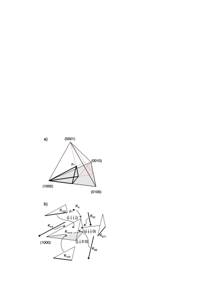
FIG. 2.: The simplex of eigenvalues of the $N=4$ density matrices (a). Pure states are represented by four corners of the thetrahedron, while its center denotes the maximally mixed state $\rho_{*}$. Magnification of the asymmetric part od the simplex, related to the Weyl chamber (b). It can be decomposed into $8$ parts according to different kinds of degeneracy of the spectrum.

Note that the unitary matrix of eigenvectors $V$ is not determined uniquely, since $W=VRV^{\dagger}=VHRH^{\dagger}V^{\dagger}$, where $H$ is an arbitrary diagonal unitary matrix. This stability group of $U$ is parametrized by $N=4$ independent phases. Thus for a generic case of all eigenvalues $r_{i}$ different, (which corresponds to the interior $K_{1111}$ of the simplex), the space of global orbits has a structure of the quotient group $U(4)/[U(1)^{4}]$. It has $D_{g}=16-4=12$ dimensions.

If degeneracy in the spectrum of $W$ occurs, say $r_{1}=r_{2}>r_{3}>r_{4}$, than the stability group $H=U(2)\times U(1)\times U(1)$ is $4+1+1=6$ dimensional [24]. In this case, corresponding to the face $K_{211}$ of the simplex, the global orbit $U/H$ has $D_{g}=16-6=10$ dimensions. The dimensionality is the same for the other faces of the simplex, $K_{121}$ and $K_{112}$. The important case of pure states corresponds to the triple degeneracy, $r_{1}>r_{2}=r_{3}=r_{4}$ for which the stability group $H$ equals $U(3)\times U(1)$. The orbits $U/H=SU(4)/U(3)$ have a structure of complex projective space ${\mathbb{C}}P^{3}$. This $6$D manifold results thus of all points of the Weyl chamber located at the edge $K_{13}$. These parts of the asymmetric simplex are shown in Fig.2, the indices labeling each part give the number of degenerated eigenvalues in decreasing order. For another edge $K_{22}$ of the simplex $H=U(2)\times U(2)$ and the quotient group $U/H$ is $16-8=8$ dimensional. In the last case of quadruple degeneracy, corresponding to the maximally mixed state $\rho_{*}={\hbox{\Bbb I}}/4$, the stability group $H=U(4)$, thus $D_{l}=0$. A detailed description of the decomposition of the Weyl chamber with respect to the dimensionality of global orbits for arbitrary dimensions is provided in [25].

C Dimensionality of local orbits

For $K=M=2$ (two qubit system) $c_{ijk}=-2\epsilon_{ijk}$ and $d_{\alpha\beta\gamma}=-2\epsilon_{\alpha\beta\gamma}$, where $\epsilon_{\alpha\beta\gamma}$ is completely antisymetric tensor. Formulae (15) give in this case

$$A=8[(\text{Tr}G^{\prime}G^{\prime T})\cdot I-G^{\prime}G^{\prime T}]+8(\|\bf{a^{\prime}}\|^{2}\cdot I-{\bf a^{\prime}}{\bf a^{\prime}}^{T}),$$ (33)

$$D=8[(\text{Tr}G^{\prime}G^{\prime T})\cdot I-G^{\prime T}G^{\prime}]+8(\|\bf{b^{\prime}}\|^{2}\cdot I-{\bf b^{\prime}}{\bf b^{\prime}}^{T}),$$ (34)

and

$$BG^{\prime T}=G^{\prime T}B=-16\;\text{det}G^{\prime}\cdot I,$$ (35)

where $3D$ vectors $\bf a^{\prime}$, $\bf b^{\prime}$ and a $3\times 3$ matrix $G^{\prime}$ represent a certain $N=4$ mixed state $W$ in the form (7). For later convenience we denote the system variables by symbols with primes. For $\text{det}G^{\prime}\neq 0$ the last equation gives $B=-16\text{det}G^{\prime T}\cdot(G^{\prime T})^{-1}$, but below we will show the more convenient representation of $B$.

Since $G^{\prime}$ is real, we can find its singular value decomposition in terms of two real orthogonal matrices $O_{1}$, $O_{2}$ and a positive diagonal matrix

$$O_{1}G^{\prime}O_{2}^{T}=G=\left[\begin{array}[]{ccc}\mu_{1}&0&0\\ 0&\mu_{2}&0\\ 0&0&\mu_{3}\end{array}\right],\quad\mu_{1}\geq\mu_{2}\geq\mu_{3}\geq 0.$$ (36)

If the determinant of $G^{\prime}$ is positive then one can choose $O_{1}$ and $O_{2}$ as proper orthogonal matrices (i.e. with the determinants equal to one). In this case the singular value decomposition (36) corresponds to a local transformation $W=U_{1}\otimes U_{2}W(U_{1}\otimes U_{2})^{\dagger}$. In the opposite case of a negative determinant of $G^{\prime}$ one of the matrices $O_{1},O_{2}$ has also a negative determinant. Alternatively, we can assume that $O_{1}$ and $O_{2}$ are proper orthogonal matrices (with positive determinants), and, consequently, the singular value decomposition corresponds to a local transformation, but with $\mu_{1}\leq\mu_{2}\leq\mu_{3}\leq 0$.

From (34) and (35) it follows, that the above transformation $G=O_{1}G^{\prime}O_{2}^{T}$, if supplemented by ${\bf a}=O_{1}{\bf a^{\prime}}$ and ${\bf b}=O_{2}{\bf b^{\prime}}$, induces the transformation $C=C^{\prime}(G^{\prime},{\bf a^{\prime}},{\bf b^{\prime}})\mapsto C(G,{\bf a},{\bf b})=(O_{1}\oplus O_{2})C^{\prime}(O_{1}\oplus O_{2})^{T}$, where

$$O_{1}\oplus O_{2}:=\left[\begin{array}[]{cc}O_{1}&0\\ 0&O_{2}\end{array}\right],$$ (37)

leaving the spectrum of $C$ invariant. The explicit form of the transformed matrix inferred from (34), (35), and (36) reads

$$C = \left[\begin{array}[]{cccccc}8\left(\mu_{2}^{2}+\mu_{3}^{2}\right)&0&0&\mp 16\mu_{2}\mu_{3}&0&0\\ 0&8\left(\mu_{1}^{2}+\mu_{2}^{3}\right)&0&0&\mp 16\mu_{1}\mu_{3}&0\\ 0&0&8\left(\mu_{1}^{2}+\mu_{2}^{2}\right)&0&0&\mp 16\mu_{1}\mu_{2}\\ \mp 16\mu_{2}\mu_{3}&0&0&8\left(\mu_{2}^{2}+\mu_{3}^{2}\right)&0&0\\ 0&\mp 16\mu_{1}\mu_{3}&0&0&8\left(\mu_{1}^{2}+\mu_{3}^{2}\right)&0\\ 0&0&\mp 16\mu_{1}\mu_{2}&0&0&8\left(\mu_{1}^{2}+\mu_{2}^{2}\right)\end{array}\right]$$ (44)

$$+ \left[\begin{array}[]{cc}8\left(\|{\bf a}\|^{2}\cdot I-{\bf a}({\bf a})^{T}\right)&0\\ 0&8\left(\|{\bf b}\|^{2}\cdot I-{\bf b}({\bf b})^{T}\right)\end{array}\right]:=C_{G}+C_{\bf{a},\bf{b}}$$ (47)

which is the sum of two real positive definite matrices, $C_{G}$ and $C_{\bf{a},\bf{b}}$. Their eigenvalues are, respectively

$$\rho_{1}=8(\mu_{1}+\mu_{2})^{2},\;\rho_{2}=8(\mu_{1}+\mu_{3})^{2},\;\rho_{3}=8(\mu_{2}+\mu_{3})^{2},$$ (48)

$$\rho_{4}=8(\mu_{1}-\mu_{2})^{2},\;\rho_{5}=8(\mu_{1}-\mu_{3})^{2},\;\rho_{6}=8(\mu_{2}-\mu_{3})^{2},$$ (49)

and

$$\nu_{1}=\nu_{2}=\|{\bf a}\|^{2},\;\nu_{3}=\nu_{4}=\|{\bf b}\|^{2},\;\nu_{5}=\nu_{6}=0.$$ (50)

Although two parts, $C_{G}$ and $C_{\bf{a},\bf{b}}$ of $C$, usually, do not commute and the eigenvalues $\lambda_{1}\geq\cdots\geq\lambda_{6}\geq 0$ of $C$ cannot be immediately found, we can investigate the possible orbits of submaximal dimensionalities using the fact that both $C_{G}$ and $C_{\bf{a},\bf{b}}$ are positive definite. It follows thus that the number of zero values among the eigenvalues $\lambda_{1},\ldots,\lambda_{6}$ of $C$ has to be matched by at least the same number of zeros among $\rho_{1},\ldots,\rho_{6}$ and among $\nu_{1},\ldots,\nu_{6}$, moreover the eigenvectors to the zero eigenvalues of the whole matrix $C$ are also the eigenvectors of the components $C_{G}$ and $C_{\bf{a},\bf{b}}$ (also, obvoiusly, corresponding to the vanishing eigenvalues)

The co-rank ${r^{\prime}}_{C_{G}}$ (the number of vanishing eigenvalues) of $C_{G}$ equals

$$6\quad \mu_{1}=\mu_{2}=\mu_{3}=0\Leftrightarrow G=0,$$ for (51)

$$3\quad \mu_{1}=\mu_{2}=\mu_{3}:=\mu\neq 0\Leftrightarrow G=\mu I,$$ for (52)

$$2\quad \mu:=\mu_{1}>\mu_{2}=\mu_{3}=0,$$ for (53)

$$1\quad \mu_{M}:=\mu_{1}>\mu_{2}=\mu_{3}:=\mu_{m}\neq 0,$$ for (54)

or $$0\neq\mu:=\mu_{1}=\mu_{2}>\mu_{3},$$ (55)

and is equal $0$ in all other cases, whereas for $C_{{\bf a},{\bf b}}$ it co-rank ${r^{\prime}}_{C_{{\bf a},{\bf b}}}$ reads

$$6\quad {\bf a}={\bf b}=0,$$ for (56)

$$4\quad {\bf a}=0,\;{\bf b}\neq 0\;\text{or }\;{\bf a}\neq 0,\;{\bf b}=0,$$ for (57)

$$2\quad {\bf a}\neq 0,\;{\bf b}\neq 0.$$ for (58)

As already mentioned, in a generic case all eigenvalues of the $6$D Gram matrix $C$ are positive and the dimension of local orbits is maximal, $d_{l}=6$. On the other hand, the above decomposition of the Gram matrix is very convenient to analyze several special cases, for which some eigenvalues of $C$ reduce to zero and the local orbits are less dimensional. To find all of them one needs to consider $9$ combinations of different ranks of the matrices $C_{G}$ and $C_{\bf{a},\bf{b}}$ as shown in the Appendix.

For any point of the Weyl chamber we know thus the dimension $D_{g}$ of the corresponding global orbit. Using above results for any of the globally equivalent states $W$ (with the same spectrum) we may find the dimension $D_{l}$ of the corresponding local orbit. This dimension may be state dependent, as explicitly shown for the case of $N=4$ pure states. Let $D_{m}$ denotes the maximal dimension $D_{l}$, where the maximum is taken over all states of the global orbit. The set of effectively different states, which cannot be linked by local transformations has thus dimension $D_{d}=D_{g}-D_{m}$. For example, the effectively different space of the $N=4$ pure states is one dimensional, $D_{d}=6-5=1$.

D Special case: triple degeneracy and generalized Werner states

Consider the longest edge, $K_{13}$, of the Weyl chamber, which represents a class of states with the triple degeneracy. They may be written in the form $\rho_{x}:=x|\Psi\rangle\langle\Psi|+(1-x)\rho_{*}$, where $|\Psi\rangle$ stands for any pure state and $x\in(0,1]$. The global orbits have the structure $U(4)/[U(3)\times U(1)]$, just as for the pure states, which are generated by the corner of the simplex, represented by $x=1$. Also the topology of the local orbits do not depends on $x$, and the stratification found for pure states holds for each $6$ dimensional global orbit generated by any single point of the edge.

Schematic drawing shown in Fig.1 is still valid, but now the term ”maximally entangled” denotes the entanglement maximal on the given global orbit. It decreases with $x$ as for Werner states, with $|\Psi\rangle$ chosen as the maximally entangled pure state [27]. For these states the concurrence decreases linearly, $c(x)=(3x-1)/2$ for $x>1/3$ and is equal to zero for $x\leq 1/3$. Thus for sufficiently small $x$ (sufficiently large degree of mixing) all states are separable, also these belonging to one of the both $3$D local orbits. This is consistent with the results of [5], where it was proved that if Tr$\rho^{2}<1/3$ the $2\times 2$ mixed state $\rho$ is separable.

This condition has an appealing geometric interpretation: on one hand it represents the maximal $3$D ball inscribed in the tetrahedron of eigenvalues, as shown in Fig.3. On the the other, it represents the maximal $15$D ball $B_{M}$, (in sense of the Hilbert-Schmidt metric, $D_{HS}^{2}(\rho_{1},\rho_{2})=\rm{Tr}(\rho_{1}-\rho_{2})^{2}$), contained in the $15$D set of all mixed states for $N=4$. Both balls are centered at the maximally mixed state $\rho_{*}$ (the center of the eigenvalues simplex of side $\sqrt{2}$), and have the same radius $1/2\sqrt{3}$. A similar geometric discussion of the properties of the set of $2\times 2$ separable mixed states was recently given in [26].

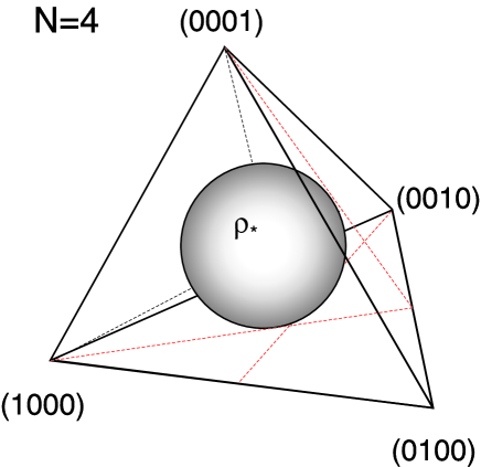
FIG. 3.: Separability of the maximal $15$D ball: all mixed states with spectra represented by points inside the ball inscribed in the $3$D simplex of eigenvalues of the $N=4$ density matrices are separable.

To clarify the structure of effectively different states in this case we consider generalized Werner states

$$\rho(x,\theta):=x|\Psi_{\theta}\rangle\langle\Psi_{\theta}|+(1-x)\rho_{*},$$ (59)

where the state $|\Psi_{\theta}\rangle:=[\cos(\theta/2),0,0,\sin(\theta/2)]$, contains the line of effectively different pure states for $\theta\in[0,\pi/2]$. Note that the case $\theta=\pi/2$ is equivalent to the original Werner states [27]. Entanglement of formation $E$ for the states $\rho(x,\theta)$ may be computed analytically with help of concurrence and the Wootters formula [14]. The results are too lengthy to be reproduced here, so in Fig.4 we present the plot $E=E(x,\theta)$. The graph is done in polar coordinates, so the pure states are located at the circle $x=1$. For each fixed $x$ the space of effectively different states is represented by a quarter of the circle. For $x<1/3$ entire circle is located inside the maximal ball $B_{M}$, and all effectively different states are separable. Points located along a circle centerd at $\rho_{*}$ represent mixed states, which are described by the same spectrum and can be connected by a global unitary transformation $U(4)$. In accordance to the recent results of Hiroshima and Ishizaka [28], the original Werner states enjoy the largest entanglement accesible by unitary operations.

The convex set $\cal S$ of separable states contains a great section of the maximal ball and touches the set of pure states in two points only. The actual shape of $\cal S$ (at this cross-section) looks remarkably similar to the schematic drawing which appeared in [6]. Moreover, the contour lines of constant $E$ elucidate important feature of any measure of entanglement: the larger shortest distance to $\cal S$, the larger entanglement [9]. Even though we are not going to prove that for any state $\rho$, its shortest distance to $\cal S$ at the picture is strictly the shortest in the entire $15$D space of mixed states, the geometric structure of the function $E=E(x,\theta)$ is in some sense peculiar: The contours $E=$const are foliated along the boundary of $\cal S$, while both maximally entangled states are located as far from $\cal S$, as possible.

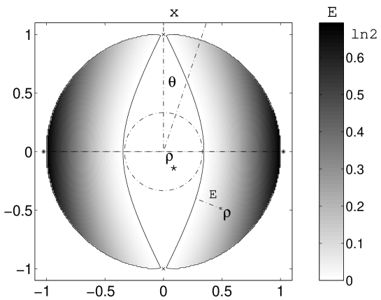
FIG. 4.: Entanglement of formation $E$ for the generalized Werner states $\rho_{x,\theta}$ represented in the polar coordinates. Intersection with the maximal ball centered at $\rho_{*}$ is separable (white). Dashed horiznotal line, joining two maximally entangled states $(*)$, (black), represents the original Werner states. Entanglement $E$ of a mixed state $\rho$ may be interpreted as its distance from the set of separable states.

E Absolutely separable states

Defining separability of a given mixed state $\rho$, we implicitly assume that the product structure of the composite Hilbert space is given, $\cal{H}=\cal{H}_{A}\otimes\cal{H}_{B}$. This assumption is well justified from the physical point of view. For example, the EPR scenario distinguishes both subsystems in a natural way (’left photon’ and ’right photon’). Then we speak about separable (entangled) states, with respect to this particular decomposition of $\cal H$. Note that any separable pure state may be considered entangled, if analyzed with respect to another decomposition of $\cal H$.

On the other hand, one may pose a complementary question, interesting merely from the mathematical point of view, which states are separable with respect to any possible decomposition of the $N=K\times M$ dimensional Hilbert space $\cal H$. More formally, we propose the following

definition. Mixed quantum state $\rho$ is called absolutely separable, if all globally similar states $\rho^{\prime}=U\rho U^{\dagger}$ are separable.

Unitary matrix $U$ of size $N$ represents a global operation equivalent to a different choice of both subsystems. It is easy to see that the most mixed state $\rho_{*}$ is absolutely separable. Moreover, the entire maximal ball $B_{M}=B(\rho_{*},1/2\sqrt{3})$ is absolutely separable for $N=4$. This is indeed the case, since the proof of separability of $B_{M}$ provided in [5] relays only on properties of the spectrum of $\rho$, invariant with respect to global operations $U$. Another much simpler proof of separability of $B_{M}$ follows directly from inequality (9.21) of the book of Mehta [29].

Are there any $2\times 2$ absolutely separable states not belonging to the maximal ball $B_{M}$? Recent results of Ishizaka and Hiroshima [30] suggest, that this might be the case. They conjectured that the maximal concurrence on the local orbit determined by the spectrum $\{r_{1},r_{2},r_{3},r_{4}\}$ is equal to $c^{*}={\rm max}\{0,r_{1}-r_{3}-2\sqrt{r_{2}r_{4}}\}$. This conjecture has been proved for the density matrices of rank $1,2$ and $3$ [30]. If it is true in the general case than the condition $c^{*}>0$ defines the $3D$ set of spectra of absolutely separable states. This set belongs to the regular tetrahedron of eigenvalues and contains the maximal ball $B_{M}$. For example, a state with the spectrum $\{0.47,0.30,0.13,0.10\}$ does not belong to $B_{M}$ but its $c^{*}$ is equal to zero.

IV Concluding remarks

In order to analyze geometric features of quantum entanglement we studied the properties of orbits generated by local transformations. Their shape and dimensionality is not universal, but depends on the initial state. For each quantum state of arbitrary $K\times M$ problem we defined the Gram matrix $C$, the spectrum of which remains invariant under local transformation. The rank of $C$ determines dimensionality of the local orbit. For generic mixed states the rank is maximal and equal to $D_{l}=K^{2}+M^{2}-2$, while the space of all globally equivalent states (with the same spectrum) is $(KM)^{2}-KM$ dimensional. Thus the set of states effectively different, which cannot be related by any local transformation, has $D_{d}=(KM)^{2}-KM-(K^{2}+M^{2}-2)$ dimensions.

For the pure states of the simplest $2\times 2$ problem we have shown that the set of effectively different states is one dimensional. This curve may be parametrized by an angle emerging in the Schmidt decomposition: it starts at a $3$D set of maximally entangled states, crosses the $5$D spaces of states of gradually decreasing entanglement, and ends at the $4$D manifold of separable states.

We presented an explicit parametrization of these submaximal manifolds. Moreover, we have proved that any pure state can be transformed by means of local transformations into one of the states at this line. In such a way we found a stratification of the $6$D manifold ${\mathbb{C}}P^{3}$ along the line of effectively different states into subspaces of different dimensionality.

Since for $N=4$ pure states the set of effectively different states is one dimensional, all measures of entanglement must be equivalent (and be functions of, say, concurrence or entropy of formation). This is not the case for generic mixed states, for which $D_{d}=6$. Hence there exist mixed states of the same entanglement of formation with the same spectrum (globally equivalent), which cannot be connected by means of local transformations.

It is known that some measures of entangled do not coincide (e.g. entanglement of formation $E$ and distillable entanglement $E_{d}$ [11]). To characterize the entanglement of such mixed states one might, in principle, use $6$ suitably selected local invariants. This seem not to be very practical, but especially for higher systems, for which the dimension $D_{d}$, of effectively different states is large and the bound entangled states exist (with $E_{d}=0$ and $E>0$), one may consider using some additional measures of entanglement. All such measures of entanglement have to be functions of eigenvalues of the Gram matrix $C$ or other invariants of local transformations [16, 15, 17, 18, 19].

We analyzed geometry of the convex set of separable states. For the simplest $N=4$ problem it contains the maximal $15$D ball, inscribed in the set of the mixed states. It corresponds to the $3$D ball of radius $1/2\sqrt{3}$ inscribed in the simplex of eigenvalues. This property holds also for $2\times 3$ problem, for which the radius is $1/\sqrt{30}$. For larger problems $K\times M=N\geq 8$, it is known that all mixed states in the maximal ball (of radius $(N(N-1))^{-1/2}$) are not distillable [5], but the question whether they are separable remains open.

Acknowledgments

It is a pleasure to thank Paweł Horodecki for several crucial comments and Ingemar Bengtsson, Paweł Masiak and Wojciech Słomczyński for inspiring discussions. One of us (K.Ż.) would like to thank the European Science Foundation and the Newton Institute for a support allowing him to participate in the Workshop on Quantum Information organized in Cambridge in July 1999, where this work has been initiated. Financial support by a research grant 2 P03B 044 13 of Komitet Badań Naukowych is gratefully acknowledged.

A Submaximal local orbits for $2\times 2$ problem

In this appendix we give the list of all possible submaximal ranks of the Gram matrix $C$ which determine the dimension of the local orbit $D_{l}=6-r_{C}$. The symbol $r^{\prime}_{X}$ denotes the co-rank, it is the number of zeros in the spectrum of $X$. In each submaximal case we provide the density matrix $W$, Gram matrix $C$ and its eigenvalues $\lambda_{i}$, $i=1,\dots,6$ expressed as a function of the the singular values of the matrix $G^{\prime}$ and the vectors ${\bf a}=O_{1}{\bf a^{\prime}}$ and ${\bf b}=O_{2}{\bf b^{\prime}}$, where orthogonal matrices $O_{1}$ and $O_{2}$ are determined by the singular value decomposition of $G^{\prime}$.

In a general case the density matrix $W=W\left(G,{\bf a},{\bf b}\right)=W\left(\mu_{1},\mu_{2},\mu_{3},a_{1},a_{2},a_{3},b_{1},b_{2},b_{3}\right)$ is given by

$$W=\ \ \frac{1}{4}I+\left[\begin{array}[]{cccc}-a_{3}-b_{3}-\mu_{3}&-b_{1}-ib_{2}&-a_{1}-ia_{2}&-\mu_{1}+\mu_{2}\\ -b_{1}+ib_{2}&-a_{3}+b_{3}+\mu_{3}&-\mu_{1}-\mu_{2}&-a_{1}-ia_{2}\\ -a_{1}+ia_{2}&-\mu_{1}-\mu_{2}&a_{3}-b_{3}+\mu_{3}&-b_{1}-ib_{2}\\ -\mu_{1}+\mu_{2}&-a_{1}+ia_{2}&-b_{1}+ib_{2}&a_{3}+b_{3}-\mu_{3}\end{array}\right]$$ (A1)

where we use the rotated basis in which $G$ is diagonal. The characteristic equation of the density matrix $W$ reads

$$\det\left(W-\varrho\right) = \varrho^{4}-\varrho^{3}+\left[\frac{3}{8}-2\left\|{\bf a}\right\|^{2}-2\left\|{\bf b}\right\|^{2}-2\text{Tr}G^{2}\right]\varrho^{2}+\left(-\frac{1}{16}+\left\|{\bf a}\right\|^{2}+\left\|{\bf b}\right\|^{2}+\text{Tr}G^{2}+8{\bf a}G{\bf b}-8\det G\right)\varrho$$ (A4)

$$+\left(\left\|{\bf a}\right\|^{2}-\left\|{\bf b}\right\|^{2}\right)^{2}+2\text{Tr}G^{4}-\left(\text{Tr}G^{2}\right)^{2}-\frac{1}{8}\left\|{\bf a}\right\|^{2}-\frac{1}{8}\left\|{\bf b}\right\|^{2}-\frac{1}{8}\text{Tr}G^{2}-2{\bf a}G{\bf b}+2\det G$$

$$-4\left\|G{\bf a}\right\|^{2}-4\left\|G{\bf b}\right\|^{2}+2\left(\left\|{\bf a}\right\|^{2}+\left\|{\bf b}\right\|^{2}\right)\text{Tr}G^{2}+8\left(a_{1}b_{1}\mu_{2}\mu_{3}+a_{2}b_{2}\mu_{1}\mu_{3}+a_{3}b_{3}\mu_{1}\mu_{2}\right)+\frac{1}{256}.$$

It is interesting to note that the characteristic equation of the partially transposed matrix $\widetilde{W}=W^{T_{2}}$ differs only by signs of three terms:

$$\det\left(W-\widetilde{\varrho}\right) = \widetilde{\varrho}^{4}-\widetilde{\varrho}^{3}+\left[\frac{3}{8}-2\left\|{\bf a}\right\|^{2}-2\left\|{\bf b}\right\|^{2}-2\text{Tr}G^{2}\right]\widetilde{\varrho}^{2}+\left(-\frac{1}{16}+\left\|{\bf a}\right\|^{2}+\left\|{\bf b}\right\|^{2}+\text{Tr}G^{2}+8{\bf a}G{\bf b}+8\det G\right)\widetilde{\varrho}$$ (A7)

$$+\left(\left\|{\bf a}\right\|^{2}-\left\|{\bf b}\right\|^{2}\right)^{2}+2\text{Tr}G^{4}-\left(\text{Tr}G^{2}\right)^{2}-\frac{1}{8}\left\|{\bf a}\right\|^{2}-\frac{1}{8}\left\|{\bf b}\right\|^{2}-\frac{1}{8}\text{Tr}G^{2}-2{\bf a}G{\bf b}-2\det G$$

$$-4\left\|G{\bf a}\right\|^{2}-4\left\|G{\bf b}\right\|^{2}+2\left(\left\|{\bf a}\right\|^{2}+\left\|{\bf b}\right\|^{2}\right)\text{Tr}G^{2}-8\left(a_{1}b_{1}\mu_{2}\mu_{3}+a_{2}b_{2}\mu_{1}\mu_{3}+a_{3}b_{3}\mu_{1}\mu_{2}\right)+\frac{1}{256}.$$

Let $\varrho_{i}$ and $\widetilde{\varrho}_{i}$, $i=1,2,3,4$, denote the eigenvalues of $W$ and $\widetilde{W}$, respectively. Due to Peres-Horodeccy partial transpose criterion [1, 2] positivity of $\widetilde{\varrho}_{i}$ may be used to find, under which conditions $W$ is separable.

In order to compute the concurrence of the density matrix $W$, let us define an auxiliary hermitian matrix

$$\overline{W}:=W\sigma_{2}\otimes\sigma_{2}W^{\ast}\sigma_{2}\otimes\sigma_{2},$$ (A8)

where ^∗ represents the complex conjugation. Let $\xi_{i}$, $i=1,2,3,4$ denote the eigenvalues of $\overline{W}$, arranged in decreasing order. Then the concurrence $c$ of $W$ is given by [13, 14]

$$c:=\max\left(0,\sqrt{\xi_{1}}-\sqrt{\xi_{2}}-\sqrt{\xi_{3}}-\sqrt{\xi_{4}}\right).$$ (A9)

The Gram matrix $C=C\left(G,{\bf a},{\bf b}\right)=C\left(\mu_{1},\mu_{2},\mu_{3},a_{1},a_{2},a_{3},b_{1},b_{2},b_{3}\right)$ corresponding to the density matrix $W$, reads in the general case

$$C=8\left[\begin{array}[]{cccccc}a_{2}^{2}+a_{3}^{2}+\mu_{2}^{2}+\mu_{3}^{2}&-a_{1}a_{2}&-a_{1}a_{3}&-2\mu_{2}\mu_{3}&0&0\\ -a_{1}a_{2}&a_{1}^{2}+a_{3}^{2}+\mu_{1}^{2}+\mu_{3}^{2}&-a_{2}a_{3}&0&-2\mu_{1}\mu_{3}&0\\ -a_{1}a_{3}&-a_{2}a_{3}&a_{1}^{2}+a_{2}^{2}+\mu_{1}^{2}+\mu_{2}^{2}&0&0&-2\mu_{1}\mu_{2}\\ -2\mu_{2}\mu_{3}&0&0&b_{2}^{2}+b_{3}^{2}+\mu_{2}^{2}+\mu_{3}^{2}&-b_{1}b_{2}&-b_{1}b_{3}\\ 0&-2\mu_{1}\mu_{3}&0&-b_{1}b_{2}&b_{1}^{2}+b_{3}^{2}+\mu_{1}^{2}+\mu_{3}^{2}&-b_{2}b_{3}\\ 0&0&-2\mu_{1}\mu_{2}&-b_{1}b_{3}&-b_{2}b_{3}&b_{1}^{2}+b_{2}^{2}+\mu_{1}^{2}+\mu_{2}^{2}\end{array}\right]$$ (A10)

Below we provide a list of the classes of states corresponding to the submaximal ranks $r_{C}$ of the Gram matrices. The list is ordered according to the increasing dimensionality of local orbits; $D_{l}=r_{C}=6-r_{C}^{\prime}$.

Case 1. $r_{C}^{\prime}=6,$  $G=0,$  ${\bf a}=0,$  ${\bf b}=0,$; $C=0$

$$\lambda_{1,2,3,4,5,6}=0;~{}~{}W=\frac{1}{4}I;~{}~{}\varrho_{1,2,3,4}=\frac{1}{4}=\widetilde{\varrho}_{1,2,3,4},~{}~{}\xi_{1,2,3,4}=\frac{1}{16},$$ (A11)

thus $W$ is separable and concurrence, $c$, is equal to zero.

Case 2. $r_{C}^{\prime}=4,$  $G=0,$  ${\bf a}\neq 0,$  ${\bf b}=0,$

$$\lambda_{1,2}=8\|{\bf a}\|^{2},~{}~{}\lambda_{3,4,5,6}=0;$$ (A12)

$$\varrho_{1,2}=\frac{1}{4}+\left\|{\bf a}\right\|,\varrho_{3,4}=\frac{1}{4}-\left\|{\bf a}\right\|;$$ (A13)

$$\widetilde{\varrho}_{1,2}=\frac{1}{4}+\left\|{\bf a}\right\|,\widetilde{\varrho}_{3,4}=\frac{1}{4}-\left\|{\bf a}\right\|.$$ (A14)

$$\xi_{1,2,3,4}=\frac{1}{16}-\left\|{\bf a}\right\|^{2},~{}~{}{\rm thus}~{}~{}c=0.$$ (A15)

$W$ represents a density matrix for $\left\|{\bf a}\right\|\leq\frac{1}{4}$ and then is separable ($\widetilde{W}\geq 0$).

Case 3. $r_{C}^{\prime}=3$; $G=\mu I,$  ${\bf a}=0,$  ${\bf b}=0,$

$$\lambda_{1,2,3}=32\mu^{2},\ \lambda_{4,5,6}=0$$ (A16)

$$\varrho_{1,2,3}=\frac{1}{4}-\mu,\ \varrho_{4}=\frac{1}{4}+3\mu,$$ (A17)

$$\widetilde{\varrho}_{1,2,3}=\frac{1}{4}+\mu,\ \widetilde{\varrho}_{4}=\frac{1}{4}-3\mu.$$ (A18)

$$\xi_{1}=\frac{1}{16}\left(12\mu+1\right)^{2},\quad\xi_{2,3,4}=\frac{1}{16}\left(1-4\mu\right)^{2},$$ (A19)

$$c=\left\{\begin{array}[]{ccc}0&\text{for}&\mu\leq\frac{1}{12}\\ 6\mu-\frac{1}{2}&\text{for}&\frac{1}{12}\leq\mu\leq\frac{1}{4}\end{array}\right.$$ (A20)

$W\geq 0$  for  $-\frac{1}{12}\leq\mu\leq\frac{1}{4}$ and $W$ is separable for $|\mu|\leq\frac{1}{12}$.

Case 4. $r_{C}^{\prime}=2$. $G=0,$

$$\lambda_{1,2}=8\|{\bf a}\|^{2},\ \lambda_{3,4}=8\|{\bf b}\|^{2},\lambda_{5,6}=0.$$ (A21)

$$\varrho_{1}=\frac{1}{4}+\left\|{\bf a}\right\|+\left\|{\bf b}\right\|,\ \varrho_{2}=\frac{1}{4}-\left\|{\bf a}\right\|-\left\|{\bf b}\right\|,\ \ \varrho_{3}=\frac{1}{4}+\left|\left\|{\bf a}\right\|-\left\|{\bf b}\right\|\right|,\ \ \varrho_{4}=\frac{1}{4}-\left|\left\|{\bf a}\right\|-\left\|{\bf b}\right\|\right|$$ (A22)

$$\widetilde{\varrho}_{1}=\frac{1}{4}+\left\|{\bf a}\right\|+\left\|{\bf b}\right\|,\ \widetilde{\varrho}_{2}=\frac{1}{4}-\left\|{\bf a}\right\|-\left\|{\bf b}\right\|,\ \ \widetilde{\varrho}_{3}=\frac{1}{4}+\left|\left\|{\bf a}\right\|-\left\|{\bf b}\right\|\right|,\ \ \widetilde{\varrho}_{4}=\frac{1}{4}-\left|\left\|{\bf a}\right\|-\left\|{\bf b}\right\|\right|.$$ (A23)

$$\xi_{1,2}=\frac{1}{16}+\left(\left\|{\bf a}\right\|+\left\|{\bf b}\right\|\right)^{2},\quad\xi_{3,4}=\frac{1}{16}+\left(\left\|{\bf a}\right\|-\left\|{\bf b}\right\|\right)^{2};\quad c=0.$$ (A24)

$W\geq 0$  for  $\left\|{\bf a}\right\|+\left\|{\bf b}\right\|\leq\frac{1}{4}$ and is then separable.

Case 5. ${r^{\prime}}_{C}=2$

$G=diag(\mu,0,0),$  ${\bf a}=\left[a,0,0\right]^{T},$  ${\bf b}=\left[b,0,0\right]^{T},$

$$\lambda_{1,2}=8\left(a^{2}+\mu^{2}\right),\quad\lambda_{3,4}=8\left(b^{2}+\mu^{2}\right),\ \ \lambda_{5,6}=0$$ (A25)

$$\varrho_{1}=\frac{1}{4}+a+b-\mu,\ \varrho_{2}=\frac{1}{4}-a+b+\mu,\ \varrho_{3}=\frac{1}{4}-a-b-\mu,\ \varrho_{4}=\frac{1}{4}+a-b+\mu,$$ (A26)

$$\widetilde{\varrho}_{1}=\frac{1}{4}+a+b-\mu,\ \widetilde{\varrho}_{2}=\frac{1}{4}-a+b+\mu,\ \widetilde{\varrho}_{3}=\frac{1}{4}-a-b-\mu,\ \widetilde{\varrho}_{4}=\frac{1}{4}+a-b+\mu.$$ (A27)

$$\xi_{1,2}=\left(\frac{1}{4}+\mu\right)^{2}-\left(a-b\right)^{2},\quad\xi_{3,4}=\left(\frac{1}{4}-\mu\right)^{2}-\left(a+b\right)^{2},\quad c=0.$$ (A28)

$W\geq 0$  for  $a=\left\|{\bf a}\right\|\leq\frac{1}{4}$, $\ b=\left\|{\bf b}\right\|\leq\frac{1}{4}$,  $|\mu|\leq\frac{1}{4}$; then $W$ is separable.

Case 6. ${r^{\prime}}_{C}=1$

$G=diag(\mu,0,0),$  ${\bf a}=\left[a,0,0\right]^{T},$

$$\lambda_{1} = 4\left(\|{\bf b}\|^{2}+\mu^{2}+\sqrt{(\mu^{2}-\|{\bf b}\|^{2})^{2}+4\mu^{2}{b}_{1}^{2}}\right)$$ (A29)

$$\lambda_{2} = 4\left(\|{\bf b}\|^{2}+\mu^{2}-\sqrt{(\mu^{2}-\|{\bf b}\|^{2})^{2}+4\mu^{2}{b}_{1}^{2}}\right)$$ (A30)

$$\lambda_{3} = 8\left(\|{\bf b}\|^{2}+\mu^{2}\right),\lambda_{4,5}=8\left(a^{2}+\mu^{2}\right),\quad\lambda_{6}=0\ \$$ (A31)

$$\varrho_{1} = \frac{1}{4}+a+\sqrt{\mu^{2}+\left\|{\bf b}\right\|^{2}-2b_{1}\mu},\ \ \varrho_{2}=\frac{1}{4}+a-\sqrt{\mu^{2}+\left\|{\bf b}\right\|^{2}-2b_{1}\mu},$$ (A32)

$$\varrho_{3} = \frac{1}{4}-a+\sqrt{\mu^{2}+\left\|{\bf b}\right\|^{2}+2b_{1}\mu},\ \ \varrho_{4}=\frac{1}{4}-a-\sqrt{\mu^{2}+\left\|{\bf b}\right\|^{2}+2b_{1}\mu},$$ (A33)

$$\widetilde{\varrho}_{1} = \frac{1}{4}+a+\sqrt{\mu^{2}+\left\|{\bf b}\right\|^{2}-2b_{1}\mu},\ \ \widetilde{\varrho}_{2}=\frac{1}{4}+a-\sqrt{\mu^{2}+\left\|{\bf b}\right\|^{2}-2b_{1}\mu},$$ (A34)

$$\widetilde{\varrho}_{3} = \frac{1}{4}-a+\sqrt{\mu^{2}+\left\|{\bf b}\right\|^{2}+2b_{1}\mu},\ \ \widetilde{\varrho}_{4}=\frac{1}{4}-a-\sqrt{\mu^{2}+\left\|{\bf b}\right\|^{2}+2b_{1}\mu},$$ (A35)

$$\xi_{1,2} = \frac{1}{16}+\mu^{2}-a^{2}-\left\|{\bf b}\right\|^{2}+\sqrt{4\left(a^{2}-\mu^{2}\right)\left\|{\bf b}\right\|^{2}+4\mu^{2}b_{1}^{2}+2\mu ab_{1}},$$ (A36)

$$\xi_{3,4} = \frac{1}{16}+\mu^{2}-a^{2}-\left\|{\bf b}\right\|^{2}-\sqrt{4\left(a^{2}-\mu^{2}\right)\left\|{\bf b}\right\|^{2}+4\mu^{2}b_{1}^{2}+2\mu ab_{1}},$$ (A37)

so $c=0$. If $W$ represents a density matrix $(W\geq 0)$ then it is separable.

Case 7. $r_{C}^{\prime}=1$

$G=\mu I,$  ${\bf b}=\xi{\bf a},$

$$\lambda_{1} = 4\left(\left(\xi^{2}-1\right)\|{\bf a}\|^{2}+\sqrt{\mu^{2}+\sqrt{16\mu^{4}+\left(\xi^{2}-1\right)^{2}\|{\bf a}\|^{2}}}\right),$$ (A38)

$$\lambda_{2} = 4\left(\left(\xi^{2}-1\right)\|{\bf a}\|^{2}+\sqrt{\mu^{2}-\sqrt{16\mu^{4}+\left(\xi^{2}-1\right)^{2}\|{\bf a}\|^{2}}}\right),$$ (A39)

$$\lambda_{3} = 4\left(\left(\xi^{2}-1\right)\|{\bf a}\|^{2}-\sqrt{\mu^{2}+\sqrt{16\mu^{4}+\left(\xi^{2}-1\right)^{2}\|{\bf a}\|^{2}}}\right),$$ (A40)

$$\lambda_{4} = 4\left(\left(\xi^{2}-1\right)\|{\bf a}\|^{2}-\sqrt{\mu^{2}-\sqrt{16\mu^{4}+\left(\xi^{2}-1\right)^{2}\|{\bf a}\|^{2}}}\right),$$ (A41)

$$\lambda_{5} = 32\mu^{2},\lambda_{6}=0$$ (A42)

$$\varrho_{1} = \frac{1}{4}-\mu+\left|\xi+1\right|\left\|{\bf a}\right\|,\ \ \varrho_{2}=\frac{1}{4}-\mu-\left|\xi+1\right|\left\|{\bf a}\right\|,$$ (A43)

$$\varrho_{3} = \frac{1}{4}+\mu+\sqrt{4\mu^{2}+\left(\xi-1\right)^{2}\left\|{\bf a}\right\|^{2}},\ \varrho_{4}=\frac{1}{4}+\mu-\sqrt{4\mu^{2}+\left(\xi-1\right)^{2}\left\|{\bf a}\right\|^{2}}$$ (A44)

$$\widetilde{\varrho}_{1} = \frac{1}{4}+\mu+\left|\xi-1\right|\left\|{\bf a}\right\|,\ \ \widetilde{\varrho}_{2}=\frac{1}{4}+\mu-\left|\xi-1\right|\left\|{\bf a}\right\|,$$ (A45)

$$\widetilde{\varrho}_{3} = \frac{1}{4}-\mu+\sqrt{4\mu^{2}+\left(\xi+1\right)^{2}\left\|{\bf a}\right\|^{2}},\ \widetilde{\varrho}_{4}=\frac{1}{4}-\mu-\sqrt{4\mu^{2}+\left(\xi+1\right)^{2}\left\|{\bf a}\right\|^{2}}$$ (A46)

$$\xi_{1} = \frac{1}{16}+\frac{\mu}{2}+5\mu^{2}-\left(\xi-1\right)^{2}\left\|{\bf a}\right\|^{2}+\mu\sqrt{4\left(\mu+1\right)^{2}-16\left(\xi-1\right)^{2}\left\|{\bf a}\right\|^{2}},$$ (A47)

$$\xi_{2} = \frac{1}{16}+\frac{\mu}{2}+5\mu^{2}-\left(\xi-1\right)^{2}\left\|{\bf a}\right\|^{2}-\mu\sqrt{4\left(\mu+1\right)^{2}-16\left(\xi-1\right)^{2}\left\|{\bf a}\right\|^{2}},$$ (A48)

$$\xi_{3,4} = \left(\frac{1}{4}-\mu\right)^{2}-(\left(\xi+1\right)^{2}\left\|{\bf a}\right\|^{2}$$ (A49)

If $W\geq 0$  i.e. $\varrho_{i}\geq 0$, $i=1,2,3,4$ then $|\mu|\leq\frac{1}{4}$ and $\widetilde{\varrho}_{i}\geq 0$, $i=1,3$, hence $W$ is nonseparable for $\ \sqrt{4\mu^{2}+\left(\xi+1\right)^{2}\left\|{\bf a}\right\|^{2}}>\frac{1}{4}-\mu\geq\left|\xi+1\right|\left\|{\bf a}\right\|$ or $\frac{1}{4}<|\xi-1|\|{\bf a}\|$.

Case 8. $r_{C}^{\prime}=1$

$G=diag(\mu_{1},\mu_{2},\mu_{2}),$  ${\bf a}=\left[a,0,0\right]^{T},$  ${\bf b}=\left[b,0,0\right]^{T},$

$$\lambda_{1,2} = 4\left(a^{2}+b^{2}+2\mu_{1}^{2}+2\mu_{2}^{2}+\sqrt{16\mu_{1}^{2}\mu_{2}^{2}+\left(a^{2}-b^{2}\right)^{2}}\right),$$ (A50)

$$\lambda_{3,4} = 4\left(a^{2}+b^{2}+2\mu_{M}^{2}+2\mu_{m}^{2}-\sqrt{16\mu_{1}^{2}\mu_{2}^{2}+\left(a^{2}-b^{2}\right)^{2}}\right),\lambda_{5}=32\mu_{2}^{2},\lambda_{6}=0$$ (A51)

$$\varrho_{1} = \frac{1}{4}-\mu_{1}+a+b,\ \ \varrho_{2}=\frac{1}{4}-\mu_{1}-a-b,$$ (A52)

$$\varrho_{3} = \frac{1}{4}+\mu_{1}+\sqrt{4\mu_{2}^{2}+\left(a-b\right)^{2}},\ \ \varrho_{4}=\frac{1}{4}+\mu_{1}-\sqrt{4\mu_{2}^{2}+\left(a-b\right)^{2}}$$ (A53)

$$\widetilde{\varrho}_{1} = \frac{1}{4}+\mu_{1}-a+b,\ \ \widetilde{\varrho}_{2}=\frac{1}{4}+\mu_{1}+a-b,$$ (A54)

$$\widetilde{\varrho}_{3} = \frac{1}{4}-\mu_{1}+\sqrt{4\mu_{2}^{2}+\left(a+b\right)^{2}},\ \ \widetilde{\varrho}_{4}=\frac{1}{4}-\mu_{1}-\sqrt{4\mu_{2}^{2}+\left(a+b\right)^{2}}$$ (A55)

$$\xi_{1,2} = \left(\frac{1}{4}-\mu_{1}\right)^{2}-\left(a+b\right)^{2},\quad\xi_{3}=\left(\sqrt{\left(\frac{1}{4}+\mu_{1}\right)^{2}-\left(a-b\right)^{2}}+2\mu_{2}\right)^{2},$$ (A56)

$$\xi_{4} = \left(\sqrt{\left(\frac{1}{4}+\mu_{1}\right)^{2}-\left(a-b\right)^{2}}-2\mu_{2}\right)^{2},$$ (A57)

If $W\geq 0$  i.e. $\varrho_{i}\geq 0$, $i=1,2,3,4$ then $|\mu_{1}|\leq\frac{1}{4}$ and $\widetilde{\varrho}_{i}\geq 0$, $i=1,3$, hence $W$ is nonseparable for $\ \sqrt{4\mu_{2}^{2}+\left(a+b\right)^{2}}>\frac{1}{4}-\mu_{1}\geq\left|a+b\right|$ or $\frac{1}{4}<b-a-\mu_{1}$.

Case 9. $r_{C}^{\prime}=1$

$G=diag(\mu_{1},\mu_{1},\mu_{2}),$  ${\bf a}=\left[0,0,a\right]^{T},$  ${\bf b}=\left[0,0,b\right]^{T}.$

$$\lambda_{1,2} = 4\left(a^{2}+b^{2}+2\mu_{1}^{2}+2\mu_{2}^{2}+\sqrt{16\mu_{1}^{2}\mu_{2}^{2}+\left(a^{2}-b^{2}\right)^{2}}\right),$$ (A58)

$$\lambda_{3,4} = 4\left(a^{2}+b^{2}+2\mu_{1}^{2}+2\mu_{2}^{2}-\sqrt{16\mu_{1}^{2}\mu_{2}^{2}+\left(a^{2}-b^{2}\right)^{2}}\right),\lambda_{5}=32\mu_{1}^{2},\lambda_{6}=0,$$ (A59)

$$\varrho_{1} = \frac{1}{4}-\mu_{2}+a+b,\ \ \varrho_{2}=\frac{1}{4}-\mu_{2}-a-b,$$ (A60)

$$\varrho_{3} = \frac{1}{4}+\mu_{2}+\sqrt{4\mu_{1}^{2}+\left(a-b\right)^{2}},\ \ \varrho_{4}=\frac{1}{4}+\mu_{2}-\sqrt{4\mu_{1}^{2}+\left(a-b\right)^{2}}$$ (A61)

$$\widetilde{\varrho}_{1} = \frac{1}{4}+\mu_{2}+a-b,\ \ \widetilde{\varrho}_{2}=\frac{1}{4}+\mu_{2}-a+b,$$ (A62)

$$\widetilde{\varrho}_{3} = \frac{1}{4}-\mu_{2}+\sqrt{4\mu_{1}^{2}+\left(a+b\right)^{2}},\ \ \widetilde{\varrho}_{4}=\frac{1}{4}-\mu_{2}-\sqrt{4\mu_{1}^{2}+\left(a+b\right)^{2}}$$ (A63)

$$\xi_{1,2} = \left(\frac{1}{4}-\mu_{2}\right)^{2}-\left(a+b\right)^{2},\quad\xi_{3}=\left(\sqrt{\left(\frac{1}{4}+\mu_{2}\right)^{2}-\left(a-b\right)^{2}}+2\mu_{1}\right)^{2},$$ (A64)

$$\xi_{4} = \left(\sqrt{\left(\frac{1}{4}+\mu_{2}\right)^{2}-\left(a-b\right)^{2}}-2\mu_{1}\right)^{2},$$ (A65)

If $W\geq 0$  i.e. $\varrho_{i}\geq 0$, $i=1,2,3,4$ then $|\mu_{2}|\leq\frac{1}{4}$ and $\widetilde{\varrho}_{i}\geq 0$, $i=1,3$, hence $W$ is nonseparable for $\ \sqrt{4\mu_{1}^{2}+\left(a+b\right)^{2}}>\frac{1}{4}-\mu_{2}\geq\left|a+b\right|$ or $\frac{1}{4}<b-a-\mu_{2}$.

Note that the the dimensionality $D_{l}$ given for each item holds for a non-zero choice of the relevant parameters. Some eigenvalues $\lambda_{i}$ may vanish under a special choice of parameters - these subcases are easy to find. There exists also symmetric cases $2^{\prime}$ and $6^{\prime}$ for which the vectors $\bf a$ and $\bf b$ are exchanged. The dimensionality of the local orbits remains unchanged, and the formulae for eigenvalues hold, if one exchanges both vectors.

REFERENCES

- [1] A. Peres, Phys. Rev. Lett. 77, 1413 (1996).
- [2] M. Horodecki, P. Horodecki, and R. Horodecki, Phys. Lett. A 223, 1 (1996).
- [3] M. Lewenstein, D. Bruss, J. I. Cirac, B. Kraus, M. Kuś, J. Samsonowicz, A. Sanpera, and R. Tarrach, J. Mod. Opt. 47, 2481 (2000).
- [4] M. Horodecki, P. Horodecki, and R. Horodecki, preprint LANL quant-ph/0006071
- [5] K. Życzkowski, P. Horodecki, A. Sanpera and M. Lewenstein Phys. Rev. A 58, 883, (1998).
- [6] K. Życzkowski, Phys. Rev. A 60, 3496 (1999).
- [7] S. L. Braunstein, C. M. Caves, R. Jozsa, N. Linden, S. Popescu, R. Schack, Phys. Rev. Lett. 83, 1054 (1999).
- [8] M. Lewenstein and A. Sanpera, Phys. Rev. Lett. 80, 2261 (1998).
- [9] V. Vedral and M. B. Plenio, Phys. Rev. A 57, 1619 (1998).
- [10] C. Witte, M. Trucks, Phys. Lett. A257, 14 (1999).a
- [11] M. Horodecki, P. Horodecki and R. Horodecki, Phys. Rev. Lett. 84, 2014 (2000).
- [12] C. H. Bennett, D. P. Di Vincenzo, J. Smolin and W. K. Wootters, Phys. Rev. A 54, 3814 (1996).
- [13] S. Hill and W. K. Wootters, Phys. Rev. Lett. 78, 5022 (1997).
- [14] W. K. Wootters, Phys. Rev. Lett. 80, 2245 (1998).
- [15] N. Linden, S. Popescu and A. Sudbery, Phys. Rev. Lett. 83, 243 (1999).
- [16] M. Grassl, M. Rötteler, and T. Beth, Phys. Rev. A 58, 1833 (1998).
- [17] B.-G. Englert and N. Metwally, J. Mod. Opt. 47, 2221 (2000).
- [18] A. Sudbery, LANL preprint quant-ph/0001115.
- [19] Y. Makhlin, LANL preprint quant-ph/0002045.
- [20] H. A. Carteret and A. Sudbery, J. Phys. A 33, 4981 (2000).
- [21] D. C. Brody and L. P. Hughston, LANL preprint quant-ph/9906086.
- [22] M. Kuś and K. Życzkowski, upublished.
- [23] A. Wawrzyńczyk, Group Representations and Special Functions, PWN, Warsaw, 1984.
- [24] M. Adelman, J. V. Corbett, and C. A. Hurst, Found. Phys. 23, 211 (1993).
- [25] K. Życzkowski and W. Słomczyński, LANL preprint quant-ph/0008016.
- [26] J. F. Du, M.J. Shi, X.Y. Zhou, and R.D. Han, Phys. Lett. A 267, 244 (2000).
- [27] R. F. Werner, Phys. Rev. A 40, 4277 (1989).
- [28] T. Hiroshima and S. Ishizaka, Phys. Rev. A 62, 44302 (2000).
- [29] M. L. Mehta, Matrix Theory, Hindustan Publishing, Delhi, 1989.
- [30] S. Ishizaka and T. Hiroshima, Phys. Rev. A 62, 22310 (2000).