Abstract

The mechanism of memory localization in extended domains is described in the framework of the parametric dissipative quantum model of brain. The size of the domains and the capability in memorizing depend on the number of links the system is able to establish with the external world.

1 Introduction

It is experimentally well established, since Lashley and Pribram [1, 2] pioneering work, that many functional activities of the brain involve extended assembly of neurons. On this basis, Pribram has introduced concepts of Quantum Optics, such as holography, in brain modeling [1]. Information is indeed observed to be spatially uniform ”in much the way that the information density is uniform in a hologram” [3]. While the activity of the single neuron is experimentally observed in form of discrete and stochastic pulse trains and point processes, the “macroscopic” activity of large assembly of neurons appears to be spatially coherent and highly structured in phase and amplitude [4, 5]. The quantum model of brain proposed in 1967 by Ricciardi and Umezawa [6] is firmly founded on such an experimental evidence. The model is in fact primarily aimed to the description of non-locality of brain functions, especially of memory storing and recalling. The mathematical formalism in which the model is formulated is the one of Quantum Field Theory (QFT) of many body systems. In one of his last papers [7] Umezawa explains the motivation for using QFT: ”In any material in condensed matter physics any particular information is carried by certain ordered pattern maintained by certain long range correlation mediated by massless quanta. It looked to me that this is the only way to memorize some information; memory is a printed pattern of order supported by long range correlations…If I could know what kind of correlation, I would be able to write down the Hamiltonian, bringing the brain science to the level of condensed matter physics.” The main ingredient of the model is thus the mechanism of spontaneous breakdown of symmetry by which long range correlations (the Nambu-Goldstone (NG) boson modes) are dynamically generated in many body physics. In the model the ”dynamical variables” are identified [8] with those of the electrical dipole vibrational field of the water molecules [9, 10] and of other biomolecules present in the brain structures, and with the ones of the associated NG modes, named the dipole wave quanta (dwq) [11]. The model, further developed by Stuart, Takahashi and Umezawa [12, 13] (see also [14]), exhibits interesting features related with the rôle of microtubules in the brain activity [1, 2, 8] and its extension to dissipative dynamics [11] allows a huge memory capacity. The dissipative quantum model of brain has been investigated [15] also in relation with the modeling of neural networks exhibiting long range correlations among the net units. One motivation for such a study is of course the great interest in neural network modeling, in computational neuroscience and in quantum computational strategies based on quantum evolution (quantum computation)[16].

In the present paper, we consider the parametric extension of the dissipative quantum model of brain. In previous works it has been considered the case of time independent frequencies associated to the dwq. A more general case is the one of time-dependent frequencies. The dwq may in fact undergo a number of fluctuating interactions and then their characteristic frequency may accordingly change in time. The aim of this paper is to show that dissipativity and frequency time-dependence lead to the dynamical organization of the memories in space (i.e. to their localization in more or less diffused regions of the brain) and in time (i.e. to their longer or shorter life-time).

The results we obtain agree with physiological observations which show that the neural connectivity is observed to grow as the brain develops and relates to the external world (see e.g. [17]). In the non-parametric case the region involved in memory recording (and recalling) was extending to the full system. According to the results below presented, the non-locality of memory more realistically appears now in the dynamical formations of finite size correlated ”domains”. On the other hand, the finiteness of the size of these domains implies an effective non-zero mass for the dwq and this in turn implies the appearance of related time-scales for the dwq propagation inside the domain. The arising of these time-scales seems to match physiological observation of time lapses observed in gradual recruitment of neurons in the establishment of brain functions [18, 17]. Frequency time-dependence also introduces a fine structure in the decay behavior of memories, as we will see. A further result characteristic of our model is the one which shows that the psychological arrow of time points in the same direction in which point the thermodynamical arrow of time and the cosmological arrow of time (defined by the expanding Universe direction [19, 20]).

Finally, we remark that some criticisms recently advanced [21] on the use of quantum formalism in brain modeling are quite easily turned down. Such criticisms are founded on the computation of the decoherence time of the neuron and of the microtubule. Such a decoherence time is found to be many order of magnitude shorter than typical dynamical times associated with neuron activity and kink-like microtubule excitations. The ”conclusion” that neurons and microtubules are classical objects is ”then” reached. As a matter of fact, Stuart, Takahashi and Umezawa have anticipated such a ”discovery” noticing [12], with a pleasant sense of humor, that ”it is difficult to consider neurons as quantum objects”. A careful reading of the literature thus shows that, since 1967 [6], the conclusion of ref. [21] was taken to be a rather obvious fact by the authors of the papers where the quantum model of brain and its developments have been discussed. The ”quantum” variables entering the formalism are the dynamical variable mentioned above, not to be confused with neurons and other cells. The neurons are purposely not even considered to be ”the fundamental units of the brain” [6].

In the following Section, where we briefly discuss some aspects of the dissipative quantum model, we will further consider some of the motivations to use QFT in brain modeling. The parametric extension, the formation of domains and finite life-time modes are discussed in Section 3 and 4. Section 5 is devoted to final comments and conclusions.

2 The dissipative quantum model of brain

In the quantum model of brain [6] memory recording is represented by the ordering induced in the ground state (”coding”) by means of the condensation of NG modes. These are dynamically generated through the breakdown of the rotational symmetry of the electrical dipoles of the water molecules and are called dipole wave quanta (dwq). The trigger of the symmetry breakdown is the external informational input. The recall mechanism is described as the excitation of dwq from the ground state under the action of an external imput similar to the one which produced the memory recording.

The macroscopic behavior of the brain is thus derived from the microscopic dynamics of quantum fields. The ”code” classifying the recorded information is identified with the ”order parameter” which is the macroscopic variable defining the system (memory) state. The high stability of memory demands that the long range correlation modes (the dwq) must be in the lowest energy state (the ground state), which also guarantees that memory is easily created and readily excited in the recall process. The long range correlations must also be quite robust in order to survive against the state of continuous electrochemical excitation of the brain and the continual response to external stimulation. At the same time, however, such electrochemical activity must also, of course, be coupled to the correlation modes. It is indeed the electrochemical activity observed by neurophysiology that provides a first response to external stimuli. The brain is then modeled [12, 13] as a ”mixed” system involving two separate but interacting levels. The memory level is a quantum dynamical level, the electrochemical activity is at a classical level. The interaction between the two dynamical levels is possible because the memory state is a macroscopic quantum state due to the coherence of the correlation modes.

In many-body physics there are many systems whose macroscopic properties must be described classically, but they can only be explained as arising from a quantum dynamics. The crystals, the superconductors, the superfluids, the ferromagnets, and in general all systems presenting observable ordered patterns are systems of this kind. Of course, any physical system is, in a trivial sense, a quantum system since any system is made by atoms which are quantum objects. But it is not in this trivial sense that the above mentioned systems are macroscopic quantum systems. The specific, not at all trivial way in which they appear to be ”macroscopic quantum systems” has to do with the dynamical origin of the macroscopic scale out of the microscopic quantum scale of the components. In other words, the macroscopic scale has to do not only with the large number of constituents assembled in the system (trivial summing up). This is a necessary, but not sufficient condition. The ”emergence” of the macroscopic scale has to do primarily with the appearance of long range correlations among the microscopic constituents. Due to such correlations the rate of quantum fluctuations is negligible and the system behaves as a classic one. It is well known that long range correlation modes, and their stable coherent condensation in the lowest energy state, cannot be understood without recourse to quantum dynamics.

It is then in such a way that the ”classical” behavior of the memory state has to be understood. The density of the dwq condensed in the ground state represents the information code, namely the order parameter which is a macroscopic variable. The state appears therefore as a classically behaving macroscopic quantum state.

The problem of the coupling between the quantum dynamical level and the electrochemical level is then reduced to the problem of the coupling between two macroscopic entities. Such a coupling is analogous, for example, to the coupling between classical acoustic waves and phonons in crystals. Acoustic waves are classical waves; phonons are quantum long range modes (the elastic wave quanta). Their coupling is very well known and of course experimentally observed [22].

The interaction of the external stimulus with the brain is, in conclusion, mediated by the electrochemical response. This response sets the boundary conditions such that symmetry is broken firstly in limited regions (coherence domains). If enough energy comes into play, the coherence domain boundaries may be broken; the domains then merge into larger ordered regions with the establishment of long range correlation modes and consequent recording of the information.

We also remark that the quantum model of brain is a QFT model, not a Quantum Mechanics (QM) model. QFT is dramatically different from QM. In fact the von Neumann theorem states that all the representations of the canonical commutation relations are unitary equivalent (and therefore physically equivalent) in systems with a finite number of degrees of freedom, and therefore in QM. On the contrary, in QFT the number of degrees of freedom is infinite, the von Neumann theorem thus does not hold and there exist infinitely many unitarily inequivalent representations of the canonical commutation relations. It is because of the existence of the infinitely many unitarily inequivalent representations that in QFT a system may be in different physical phases , spontaneous symmetry breakdown can occur and dynamically generated ordering sustained by long range correlations may exist in a stable state. Only in QFT it is possible to describe ”macroscopic quantum systems”. These phenomena do not occur in QM. It is also known that the source of the non-perturbative nature of many phenomena resides in the manifold of inequivalent representations of QFT. The decoherence mechanisms studied in QM have thus no relation with the coherence mechanism studied in QFT. This is the founding basis of the QFT formalism used in the quantum brain model. Therefore, one can have ordered (memory) states, which are at the same time degenerate ground states, and thus stable states for the system. This last fact would be in se a strong motivation to use QFT in brain modeling (as in fact it was for Umezawa, cf. Section 1). It can be also shown [10] that the time scale associated with the coherent interaction in the QFT of electrical dipole fields for water molecules is of the order of $10^{-14}$ $sec$, thus much shorter than times associated with short range interactions, and therefore these effects are well protected against thermal fluctuations.

By taking into account the intrinsic dissipative character of the brain dynamics, namely that the brain is an open system continuously linked with (coupled to) the environment, the memory capacity can be shown [11] to be enormously enlarged, thus solving one of the main problems left unsolved in the original formulation of the quantum brain model. To see this let us denote the dwq variables by $A$ and recall that the canonical formalism for dissipative systems requires the introduction of a “mirror” set of dynamical variables, say $\tilde{A}$. The number ${\cal{N}}_{A}$ of $A$-modes, condensed in the vacuum, constitutes the “code” of the information. The vacuum state is defined to be the state in which the difference ${\cal{N}}_{A}-{\cal{N}}_{\tilde{A}}$ is zero. There are thus infinitely many ground states, each one corresponding to a different value of the code ${\cal{N}}_{A}$. The ”brain (ground) state” may be represented as the collection (or the superposition) of the full set of memory states ${|0>}_{\cal N}$, for all $\cal N$.

The brain is thus described as a complex system with a huge number of macroscopic states (the memory states). The degeneracy among the vacua ${|0>}_{\cal N}$ plays a crucial rôle in solving the problem of memory capacity. The dissipative dynamics introduces $\cal N$-coded ”replicas” of the system and information printing can be performed in each replica without destructive interference with previously recorded informations in other replicas. A huge memory capacity is thus achieved [11].

As we will see the parametric extension of the dissipative quantum model leads to the formation of correlated domains of finite size, and to a fine structure in the life-time of the $A$ modes.

3 The parametric extension of the dissipative model and the Bessel equations

As mentioned above, in the dissipative model the canonical formalism requires the doubling of the system degrees of freedom [11]. Thus we are led to consider a couple of damped harmonic oscillators describing the system variable and its doubled, or mirror image. In the parametric model the associate frequency is assumed to be time-dependent [23]. The equations are then:

$$\stackrel{{\scriptstyle..}}{{u}}\,+\,L\stackrel{{\scriptstyle.}}{{u}}\,+\,{\omega_{n}}^{2}(t)u\,= \ 0,$$

$$\stackrel{{\scriptstyle..}}{{v}}\,-\,L\stackrel{{\scriptstyle.}}{{v}}\,+\,{\omega_{n}}^{2}(t)v\,= \ 0,$$ (1)

where:

$$\omega_{n}(t)\ =\ {\omega}_{0}\ e^{-\frac{Lt}{2n+1}}.$$ (2)

The quantities $u,v$ and $\omega_{0}$ are considered for fixed momentum $k$. $u$ and $v$ are related with the $A$ and $\tilde{A}$ modes when quantization is performed. In the following we will comment on the assumed exponential time-dependence of the frequency $\omega_{n}(t)$. Note that $\omega_{n}(t)$ approaches to the time-independent value $\omega_{0}$ for $n\rightarrow\infty$: the frequency time-dependence is thus ”graded” by $n$. We will see that $n$ has an interesting physical interpretation. $L$ is a characteristic parameters of the system. Remarkably, it is found that the couple of equations (1) is equivalent to the the spherical Bessel equation of order $n$ ($n$ is integer or zero):

$$z^{2}\ {d^{2}\over{dz}^{2}}M_{n}+2z\ {d\over{dz}}M_{n}+[z^{2}-n(n+1)]\ M_{n}\ =\ 0~{}.$$ (3)

As it is well known, Eq. (3) admits as solutions a complete set of (parametric) decaying functions [24, 25]; particular solutions are the first and second kind Bessel functions, or their linear combinations (the Hankel functions).

Note that both $M_{n}$ and $M_{-(n+1)}$ are solutions of the same eq. (3). By using the substitutions: $w_{n,l}=M_{n}\ \cdot(x_{n})^{-l}$, $z=\epsilon_{n}x_{n}$ and $x_{n}=e^{-t/\alpha_{n}}$, where $\epsilon_{n},\alpha_{n}$ are arbitrary parameters, eq.(3) goes into the following one:

$$\stackrel{{\scriptstyle..}}{{w}}_{n,l}\ -\ \frac{2l+1}{\alpha_{n}}\ \stackrel{{\scriptstyle.}}{{w}}_{n,l}+\left[\frac{l(l+1)-n(n+1)}{\alpha^{2}_{n}}\ +\ (\frac{\epsilon_{n}}{\alpha_{n}})^{2}\ e^{-2t/\alpha_{n}}\right]\ w_{n,l}\ =\ 0,$$ (4)

where $\stackrel{{\scriptstyle.}}{{w}}$ denotes derivative of $w$ with respect to time. Making the choice $l(l+1)=n(n+1)$ the degeneracy between the solutions $M_{n}$ and $M_{-(n+1)}$ is removed and two different equations are obtained, one for $l=n$ and the other one for $l=-(n+1)$ ($l$ plays the rôle of a “mirror” index):

$$\stackrel{{\scriptstyle..}}{{w}}_{n,-(n+1)}\ +\ \frac{2n+1}{\alpha_{n}}\ \stackrel{{\scriptstyle.}}{{w}}_{n,-(n+1)}+[(\frac{\epsilon_{n}}{\alpha_{n}})^{2}\ e^{-2t/\alpha_{n}}]\ w_{n,-(n+1)}\ =\ 0,$$

$$\stackrel{{\scriptstyle..}}{{w}}_{n,n}\ -\ \frac{2n+1}{\alpha_{n}}\ \stackrel{{\scriptstyle.}}{{w}}_{n,n}+[(\frac{\epsilon_{n}}{\alpha_{n}})^{2}\ e^{-2t/\alpha_{n}}]\ w_{n,n}\ =\ 0~{}.$$ (5)

By setting $u\equiv{w}_{n,-(n+1)},$ and $v\equiv{w}_{n,n}$, and choosing the arbitrary parameters $\alpha_{n}$ and $\epsilon_{n}$ in such a way that $\frac{2n+1}{\alpha_{n}}\equiv L$ and $\frac{\epsilon_{n}}{\alpha_{n}}\equiv\omega_{0}$ do not depend on $n$ (and on time), we see that eq. (5) are nothing else than the couple of eqs. (1) of the dissipative model with time-dependent frequency $\omega_{n}(t)$.

We note that $\alpha_{-(n+1)}=-\alpha_{n}$ and that the transformation $n\rightarrow-(n+1)$ leads to solutions (corresponding to $M_{-(n+1)}$) which we will not consider since they have frequencies which are exponentially increasing in time (cf. eq. (2)). These solutions can be respectively obtained from the ones of eq. (1) by time-reversal $t\rightarrow-t$.

We finally note that the functions $w_{n,n}$ and $w_{n,-(n+1)}$ are ”harmonically conjugate” functions in the sense that they may be represented as $w_{n,-(n+1)}(t)={1\over{\sqrt{2}}}r_{n}(t)e^{{-Lt\over 2}}$,  $w_{n,n}(t)={1\over{\sqrt{2}}}r_{n}(t)e^{{Lt\over 2}}$, respectively, with ${r}_{n}$ satisfying the parametric oscillator equation

$$\stackrel{{\scriptstyle..}}{{r}}_{n}+\Omega_{n}^{2}(t)r_{n}=0~{},$$ (6)

$$\Omega_{n}(t)=\left[\left({\omega}_{n}^{2}(t)-{{L^{2}}\over{4}}\right)\right]^{1\over{2}}.$$ (7)

The quantization of the system (1) can be now performed along the same line presented in refs. ([19, 23, 26, 27]). The main feature of the dissipative quantization is the “foliation” of the representations [26]. Namely, at each time $t$ the system ground state is labeled by $t$, $|0(t)>$, so that at $t^{\prime}\neq t$ the ground state $|0(t^{\prime})>$ is unitary inequivalent to $|0(t)>$: in its time evolution the system runs over unitarily inequivalent representations. The generator of such a non-unitary time evolution is found to be related to the entropy variation rate, as it should be expected since dissipation implies irreversibility [26]. We thus see that the arrow of time naturally emerges in the dissipative quantum model. Moreover, it can be shown that the system ground state is also a thermal state [26, 11], and the arrow of time due to dissipation is actually concord with the thermodynamical arrow of time (pointing in the increasing entropy direction). It has been shown [19] that both these arrows point in the same direction of the cosmological arrow of time.

We remark that the dissipative time evolution cannot be described in the framework of Quantum Mechanics, since there all the representations are unitarily equivalent due to the von Neumann theorem (cf. Section 2). Thus the motivation to use QFT in brain modeling is reinforced.

In the infinite volume limit, due to the representation unitary inequivalence, any transition among degenerate vacua would be strictly forbidden. However, in realistic conditions non-unitary time evolution and realistic phase transitions are possible due to boundary effects which ”smooth out” the infinite volume limit and inequivalence among representations is accordingly also smoothed out. We thus observe the appearance of boundaries, namely of finite size domains. This is discussed in some more details in the next section.

Finally, let us observe that the time-dependence of the frequency $\Omega_{n}$ of the coupled systems means that energy is not conserved in time and therefore that the $A-{\tilde{A}}$ system does not constitute a ”closed” system. However, when $n\rightarrow\infty$, $\Omega_{n}$ approaches to a time independent quantity, which means that energy is conserved in such a limit, i.e. the $A-{\tilde{A}}$ system gets ”closed” in that limit. Thus, in the limit $n\rightarrow\infty$ the possibilities of the system $A$ to couple to ${\tilde{A}}$ (the environment) are ”saturated”: the system $A$ gets fully coupled to $\tilde{A}$. This suggests that $n$ represents the number of links between $A$ and ${\tilde{A}}$. When $n$ is not very large (infinity), the system $A$ (the brain) has not fulfilled its capability to establish links with the external world (represented by $\tilde{A}$). On the other hand, as already mentioned, from eq.(2) we also see that $n$ “graduates” the exponential dependence on time of the frequency $\omega_{n}(t)$, namely the rate of variations in time of the frequency, or, equivalently, the ”rapidity” of the system response to external stimuli. This has been the reason for our assumption of the exponential dependence on time of the frequency $\omega_{n}(t)$.

3.1 Domains and Life-time

We observe that in order the memory recording may occur, the frequency (7) has to be real. Such a reality condition is found to be satisfied only in a definite span of time, i.e., upon restoring the suffix $k$, for times $t$ such that $0\leq t\leq T_{k,n}$, with $T_{k,n}$ given by

$$T_{k,n}\,=\,\frac{2n+1}{L}\ \ln\left(\frac{2\omega_{0,k}}{L}\right).$$ (8)

Thus, the memory recording processes can occur in limited time intervals which have $T_{k,n}$ as the upper bound, for each $k$. For times greater than $T_{k,n}$ memory recording cannot occur. Note that, for fixed $k$, $T_{k,n}$ grows linearly in $n$, which means that the time span useful for memory recording (the ability of memory storing) grows as the number of links which the system is able to lace with the external world grows: more the system is ”open” to the external world (more are the links), better it can memorize (high ability of learning).

We can also see that a threshold exists for the $k$ modes of the memory process. In fact, the reality condition ${\Omega_{k,n}}^{2}(t)\geq 0$ implies that $k\geq{\tilde{k}}(n,t)\equiv k_{0}e^{{{L\over{2n+1}}t}}$, with $k_{0}\equiv{L\over{2c}}$ at any given $t$ (note that $\omega_{0}=kc$). Note that such a kind of ”sensibility” to external stimuli only depends on the internal parameter $L$.

We remark that this intrinsic infrared cut-off precludes infinitely long wave-lengths (infinite volume limit). In fact only wave-length smaller than or equal to the cut-off ${\tilde{\lambda}}\propto{1\over{{\tilde{k}}(n,t)}}$ are allowed. This means that (coherent) domains of sizes less or equal to ${\tilde{\lambda}}$ are involved in the memory recording, and that such a cut-off shrinks in time for a given $n$. On the other hand, a growth of $n$ opposes to such a shrinking. These cut-off changes correspondingly reflect on the memory domain sizes. This also implies that transitions through different vacuum states (which would be unitarily inequivalent vacua in the infinite volume limit) at given $t$’s become possible. As a consequence, both the phenomena of association of memories and of confusion of memories, which would be avoided in the regime of strict unitary inequivalence among vacua (in the infinitely long wave-length regime), become possible [11].

Figure 1: “Lives” of $k$ modes, for fixed $n$

We can estimate the domain evolution by introducing the quantity $\Lambda_{k,n}(t)$[27, 19]:

$$e^{-2\Lambda_{k,n}(t)}\ =\ \frac{e^{-t\frac{L}{2n+1}}\,{\rm sinh}\frac{L}{2n+1}({\rm T}_{k,n}-t)}{{\rm sinh}\frac{L}{2n+1}{\rm T}_{k,n}},\qquad\,\Lambda_{k,n}(t)\ \geq 0,\,{\rm for\;any\;~{}t}~{},$$ (9)

i.e. $\Lambda_{k,n}(0)=0$ for any $k$, and $\Lambda_{k,n}(t)\rightarrow\infty$ for $t\rightarrow\ T_{k,n}$ for any given $n$. Then $\Omega_{k,n}$ may be expressed in the form:

$${\Omega_{k,n}(\Lambda_{k,n}(t))}\,=\,\Omega_{k,n}(0)e^{-\Lambda_{k,n}(t)}~{}.$$ (10)

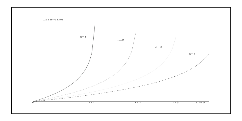
Figure 2: “Lives” of $k$ modes, for growing $n$ and fixed $k$

Since ${\Omega_{k,n}(\Lambda_{k}({\rm T}_{k,n}))}\,=\,0$, we see that $\Lambda_{k,n}(t)$ acts as a life-time, say $\tau_{k,n}$, with $\Lambda_{k,n}(t)\propto\tau_{k,n}$, for the mode $k$. Modes with larger $k$ have a ”longer” life with reference to time $t$. In other words, each $k$ mode ”lives” with a proper time $\tau_{k,n}$, so that the mode is born when $\tau_{k,n}$ is zero and it dies for $\tau_{k,n}$ $\rightarrow$ $\infty$.

The ”lives” of the $k$ modes are sketched in the figures 1-2. In Fig.1 the lives are drawn for growing $k$ and fixed $n$; vice-versa, in Fig.2, they are drawn for growing $n$ and fixed $k$. The $\Lambda_{k,n}$s are drawn versus $t$, reaching the blowing up values in correspondence of the abscissa points $T_{k,n}$. Only the modes satisfying the reality condition are present at certain time $t$, being the other ones decayed. This introduces an hierarchical organization of memories depending on their life-time: memories with a specific spectrum of $k$ mode components may coexist, some of them ”dying” before, some other ones persisting longer. As observed above, since smaller or larger $k$ modes correspond to larger or smaller waves lengths, respectively, the (coherent) associated memory domain sizes are correspondingly larger or smaller.

4 Final remarks and conclusions

In our model the processes of learning are each other independent, so it is possible that the ability in information recording may be different under different circumstances, at different ages, and so on. An interesting feature of the model which emerges from our discussion is that a higher or lower degree of openness (measured by $n$) to the external world may indeed produce a better or worse ability in learning, respectively (e.g. during the childhood or the older ages, respectively). We have also seen that the memory non-locality is ”graded” by $n$ and by the spectrum of their $k$ modes components. These also control the memory life-time or persistence: more persistent memories (with a spectrum more populated by the higher $k$ components) are also more ”localized” than shorter term memories (with a spectrum more populated by the smaller $k$ components), which instead extend over larger domains. It is thus expected that, for given $n$, ”more impressive” is the external stimulus (i.e. stronger is the coupling with the external world) greater is the number of high $k$ momentum excitations produced in the brain and more ”focused” is the ”locus” of the memory.

The qualitative behaviors and results above presented appear to fit well with the physiological observations [17] of the formation of connections among neurons as a consequence of the establishment of the links between the brain and the external world. More the brain relates to external environment, more neuronal connections will form. Connections appear thus more important in the brain functional development than the single neuron activity. Here we are referring to functional or effective connectivity, as opposed to the structural or anatomical one [17]. In fact, while the last one can be described as quasi-stationary, the former one is highly dynamic with modulation time-scales in the range of hundreds of milliseconds [17]. Once these functional connections are formed, they are not necessarily fixed. On the contrary, they may quickly change in a short time and new configurations of connections may be formed extending over a domain including a larger or a smaller number of neurons. Such a picture finds a possible description in our model, where the coherent domain formation, size and life-time depend on the number of links that the brain sets with its environment and on internal parameters.

The finiteness of the domain size also implies a non-zero effective mass of the dwq. These therefore propagate through the domain with a greater “inertia” than in the case of infinite volume where they are massless. The domain correlations are consequently established with a certain time-delay. This is also in agreement with physiological observations showing that the recruitment of neurons in a correlated assembly is achieved with a certain delay after the external stimulus action [18, 17]. In connection with the recall mechanism, we note (see ref. [11]) that the dwq effective non-zero mass acts as a threshold in the excitation energy of dwq so that, in order to trigger the recall process an energy supply equal or greater than such a threshold is required. When the energy supply is lower than the required threshold a ”difficulty in recalling” may be experienced. At the same time, however, the threshold may positively act as a ”protection” against unwanted perturbations (including thermalization) and cooperate to the stability of the memory state. In the case of zero threshold (infinite size domain) any replication signal could excite the recalling and the brain would fall in a state of ”continuous flow of memories”.

Finally, we note that after information has been recorded, the brain state is completely determined and the brain cannot be brought to the state in which it was before the information printing occurred. Thus, one is actually obliged to consider the dissipative, irreversible time-evolution: the same fact of getting information introduces the arrow of time into brain dynamics. In other words, it introduces a partition in the time evolution, namely the distinction between the past and the future, a distinction which did not exist before the information recording. It can be shown that dissipation and the frequency time-dependence imply that the evolution of the memory state is controlled by the entropy variations [11]: this feature reflects indeed the irreversibility of time evolution (breakdown of time-reversal symmetry). The stationary condition for the free energy functional leads [11] then to recognize the memory state $|0(t)>_{\cal N}$ to be a finite temperature state [28], which opens the way to the possibility of thermodynamic considerations in the brain activity. In this connection we observe that the “psychological arrow of time”, naturally emerging in the brain dynamics, turns out to point in the same direction of the “thermodynamical arrow of time”, which points in the increasing entropy direction, and of the ”cosmological arrow of time”, defined by the expanding Universe direction [20].

References

- [1] K.H.Pribram, Brain and perception, Lawrence Erlbaum, New Jersey, 1991
- [2] K.H.Pribram, Languages of the brain, Englewood Cliffs, New Jersey, 1971
- [3] W.J.Freeman, in H.Haken and M.Stadler (Eds.), Synergetics of cognition, 45, p.26, Springer Verlag, Berlin, 1990.
- [4] W.J.Freeman, Intern. J. of Neural Systems 7, 473 (1996)
- [5] W.J.Freeman, Neurodynamics: An exploration of mesoscopic brain dynamics, Springer, N.Y., 2000
- [6] L.M.Ricciardi and H.Umezawa, Kibernetik 4, 44 (1967)
- [7] H.Umezawa, Math. Japonica 41, 109 (1995)
- [8] M.Jibu , K.H.Pribram and K.Yasue, Int. J. Mod. Phys. B10, 1735 (1996)
- [9] E.Del Giudice, S.Doglia, M.Milani and G.Vitiello, Nucl. Phys. B251 [FS 13], 375 (1985); Nucl. Phys. B275 [FS 17], 185 (1986)
- [10] E.Del Giudice, G. Preparata and G. Vitiello, Phys. Rev. Lett. 61, 1085 (1988)
- [11] G. Vitiello, Int. J. Mod. Phys. 9, 973 (1995)
- [12] C.I.J.Stuart, Y.Takahashi and H.Umezawa, J. Theor. Biol. 71, 605 (1978)
- [13] C.I.J.Stuart, Y.Takahashi and H. Umezawa, Found. Phys. 9, 301 (1979)
- [14] S. Sivakami and V. Srinivasan, J. Theor. Biol. 102, 287 (1983)
- [15] E.Pessa and G.Vitiello, Biolectrochemistry and bioenergetics 48, 339 (1999)
- [16] C.J.Williams and S.H.Clearwater, Explorations in quantum computing, Springer-Verlag, New York, 1998
- [17] S.A.Greenfield, Communication and Cognition 30, 285 (1997)
- [18] B.Libet, E.W.Wright, B.Feinstein and D.K.Pearl, Brain 102, 193 (1979)
- [19] E.Alfinito, R.Manḱa and G.Vitiello, Class.Quant.Grav 17, 93 (2000)
-
[20]
S.W.Hawking Phys. Rev. D32, 2389
(1985)
S.W.Hawking and R.Penrose, The Nature of Space and Time (Princeton University Press 1996) - [21] M.Tegmark, Phys. Rev. E61, 4194 (2000)
- [22] J.P.Wolfe, J.P. Imaging phonons, Cambridge University Press, Cambridge, 1998
- [23] E.Alfinito, G. Vitiello, Formation and Life-time of memory domains in the dissipative quantum model in press on Int. J. Mod. Phys.B, quant-ph/0002014
- [24] M.Abramowitz and I.A.Stegun, Handbook of Mathematical Functions, Dover Pub. N.Y., 1970
- [25] J.D.Jackson, Classical Electrodynamics, Wiley and Sons., 1975
- [26] E. Celeghini, M. Rasetti and G. Vitiello, Annals of Phys. (N.Y.) 215, 156 (1992)
- [27] E. Alfinito and G. Vitiello Phys. Lett. A252, 5 (1999)
- [28] H.Umezawa, Advanced field theory: micro, macro and thermal concepts, American Institute of Physics, N.Y., 1993