Strongly focused light beams interacting with single atoms in free space

Abstract

We construct 3-D solutions of Maxwell’s equations that describe Gaussian light beams focused by a strong lens. We investigate the interaction of such beams with single atoms in free space and the interplay between angular and quantum properties of the scattered radiation. We compare the exact results with those obtained with paraxial light beams and from a standard input-output formalism. We put our results in the context of quantum information processing with single atoms.

I Motivation

The ability to manipulate small quantum systems individually is a necessary requirement for quantum computing and quantum communication. For example, in order to perform single-qubit operations on a particular ion in an ion trap quantum computer [1, 2, 3] one has to focus a laser beam to the position of that ion with a sufficiently high spatial resolution [4]. Similarly, quantum communication protocols using atoms trapped inside optical cavities [5, 6] require single-bit and two-bit operations on specific atoms. One question that arises is whether strong focusing has an undesired side effect, namely, that the scattered light contains information about the state of the qubit. The fear would be that the laser intensity would have to be turned down so much, that the absence of a photon from the laser beam becomes in principle detectable.

Conversely, if an atom in free space would indeed be able to modify appreciably the state of a light field, then this effect could be used to our advantage: a single atom could be used to perform quantum-logic operations on single photons in free space [7]. An atom inside an optical cavity strongly coupled to a cavity mode is known to be able to perform such tasks [8], but such an experiment would be more straightforward to conduct in free space.

At first sight the prospects of such an experiment seem good: the scattering cross section of a two-level atom is $\sigma=3\lambda^{2}/(2\pi)$ for light of wavelength $\lambda$ [9], and thus focusing light down to an area $A<\sigma$ should be sufficient to induce a strong coupling. However, this picture is too simplistic. Light beams are transversely polarized, which implies that only part of the light entering the interaction region will carry the polarization that the atom is sensitive to. Using a different picture, since the atom would emit a dipole pattern (in a given $m\rightarrow m^{\prime}$ transition), it would be most efficiently excited by a field matching an “incoming” dipole field, as follows from time-reversal symmetry. Since a focused laser beam does not have a large overlap with such a dipole pattern, the effective absorption cross section is smaller than indicated by $\sigma$.

Early experiments [10, 11] on the detection of single atom fluorescence did not reach the strong focusing limit of $A\sim\lambda^{2}$. Recently, however, impressive progress has been made in experiments on single molecules in condensed matter and efficient detection of the fluorescence light has become possible [12, 13, 14]. Experiments on single atoms aiming at the strong focusing limit are underway as well[15].

In a recent paper [16] we gave the results of explicit calculations on the behavior of single atoms in free space irradiated by tightly focused light beams. We were particularly interested in the quantum aspects of the scattered light, and in evaluating how much a single atom is able to modify the intensity and phase properties of the incident light. Here we present all the details of that calculation and discuss possible extensions. These results will be compared with similar calculations using (i) paraxial Gaussian beams [17] and (ii) a well-known quantum-optical input-output formalism that was used in Refs. [18, 19] to study photon statistics and intensity correlations of the field emitted by an atom in free space. The latter model is basically a quasi one-dimensional model, with one spatial variable describing the propagation of the light beam, and with one additional parameter describing the solid angle subtended by the laser beam at the atom’s position (coinciding with the focal point of the light beam). As we will demonstrate, however, neither this model nor, as expected, paraxial beams accurately represent the case of a strongly focused light beam.

II Strongly focused Gaussian beams

Here we wish to calculate the field that one obtains by focusing a monochromatic Gaussian (paraxial) beam by an ideal strong lens. We do that by expanding the outgoing field (i.e. the field after the lens) in a complete set of modes. In principle one can use any complete set of modes to describe exact solutions of Maxwell’s equations. In view of the cylindrical symmetry of the problem we are interested in, the most convenient is to choose a set that takes a simple form in cylindrical coordinates. In particular, we will use a set of eigenmodes of 4 commuting operators corresponding to the following 4 physical quantities: energy [with eigenvalue $\hbar kc=\hbar\omega$ per photon [20]], angular momentum in the $z$ direction [$m\hbar$], momentum in the $z$ direction [$\hbar k_{z}$], and helicity [$s\hbar k_{z}/k$]. The modes are thus characterized by the 4 numbers $\nu\equiv(k,k_{z},m,s)$, which, once the field has been quantized, play the role of quantum numbers. These modes were constructed in [21] to clarify the meaning of orbital angular momentum of light [22], and thus by construction possess simple properties under rotations around the propagation ($z$) direction. The complete orthogonal set of modes $\vec{F}_{\nu}$ is defined such that the free electric field (i.e. the solution of the source-free Maxwell equations) can be expanded in this set as

$$\vec{E}=2{\rm Re}[\sum_{\nu}a_{\nu}\vec{F}_{\nu}\exp(-i\omega t))],$$ (1)

with arbitrary complex amplitudes $a_{\nu}$. This requires the mode functions to be transverse, i.e. $\nabla\cdot\vec{F}_{\nu}=0$. The summation over $\nu$ is a short-hand notation for

$$\sum_{\nu}\equiv\int{\rm d}k\int{\rm d}k_{z}\sum_{s}\sum_{m}.$$ (2)

The dimensionless mode functions $\vec{F}_{\nu}$ in cylindrical coordinates $(\rho,z,\phi)$ are defined by[21]

$$\vec{F}_{\nu}(\rho,z,\phi) = \frac{1}{4\pi}\frac{sk-k_{z}}{k}G(k,k_{z},m+1)\hat{\epsilon}_{-}+$$ (5)

$$+\frac{1}{4\pi}\frac{sk+k_{z}}{k}G(k,k_{z},m-1)\hat{\epsilon}_{+}$$

$$-i\frac{\sqrt{2}}{4\pi}\frac{k_{t}}{k}G(k,k_{z},m)\hat{z}$$

where $k_{t}=\sqrt{k^{2}-k_{z}^{2}}$ is the transverse part of the wave vector, $\hat{\epsilon}_{\pm}=(\hat{x}\pm i\hat{y})/\sqrt{2}$ are the two circular polarization vectors, and

$$G(k,k_{z},m)=J_{m}(k_{t}\rho)\exp(ik_{z}z)\exp(im\phi),$$ (6)

with $J_{m}$ the $m$-th order Bessel function. The mode functions satisfy the orthogonality relations

$$\int{\rm d}V\vec{F}^{*}_{\nu}(\vec{r})\cdot\vec{F}_{\nu^{\prime}}(\vec{r})=\delta(k-k^{\prime})\delta(k_{z}-k_{z}^{\prime})\delta_{mm^{\prime}}\delta_{ss^{\prime}}/k,$$ (7)

where the integration extends over all space. This follows directly from the fact that the mode functions are eigenfunctions of commuting hermitian operators.

For the remainder of this Section, we will consider only monochromatic beams with a fixed value of $k=2\pi/\lambda$. For convenience we take $k_{t}$ as a mode number instead of $k_{z}$ and we denote the reduced set of mode numbers by $\mu\equiv(k_{t},m,s)$, and introduce the notation

$$\sum_{\mu}\equiv\int{\rm d}k_{t}\sum_{s}\sum_{m}.$$ (8)

For fixed $k$ the modes $\vec{F}_{\mu}$ are orthogonal in planes $z=$constant:

$$\int_{z={\rm constant}}{\rm d}S\vec{F}^{*}_{\mu}(\vec{r})\cdot\vec{F}_{\mu^{\prime}}(\vec{r})=$$ (9)

$$\delta(k_{t}-k_{t}^{\prime})\delta_{mm^{\prime}}\delta_{ss^{\prime}}/(2\pi k_{t}),$$ (10)

which is a useful relation for defining the action on light beams of an ideal lens positioned in a plane $z$=constant.

A Focusing with an ideal lens

The action of the lens is modeled here by assuming that the field distribution of the incoming field is multiplied by a local phase factor

$$\varphi=\exp(-ik\rho^{2}/2f),$$ (11)

with $f$ the focal length of the lens [23, 24]. An ideal parabolic lens would be represented by a phase factor $\varphi_{p}=\exp(ik\sqrt{\rho^{2}+(f-\rho^{2}/2f)^{2}})$. In the paraxial limit $f\gg\rho$ this factor becomes equivalent to $\varphi$. It may be that the simple lens factor used here, $\varphi$, does not give rise to the strongest possible focusing, and that $\varphi_{p}$ would improve on this. Moreover, actual lens systems designed to focus light down to $A\sim\lambda^{2}$ consist of multiple lenses (for instance, 12 in ongoing experiments [15]), partly to accommodate for the finite size, finite thickness and other imperfections of real lenses as compared to ideal lenses. We nevertheless for convenience chose a single lens factor $\varphi$: it allows for analytical evaluations and the class of light beams thus constructed does reach the focusing limit of $A\approx\sigma$ (for instance, see the plots corresponding to $f=100\lambda$). This is sufficient for our purposes of showing that even focusing down to an area of the size of the atomic cross section does not quite (by about a factor of $\sim 5$) lead to the strong effects one may have expected or hoped for.

If in the plane of the lens, say $z=0$, the incoming beam is given by

$$\vec{F}_{{\rm in}}=\vec{F}_{0}(\rho,\phi),$$ (12)

then the output field is given by

$$\vec{F}_{{\rm out}}(\vec{r})=\sum_{\mu}\kappa_{\mu}\vec{F}_{\mu}(\vec{r}),$$ (13)

with

$$\kappa_{\mu}=2\pi k_{t}\int_{z=0}{\rm d}S\exp\left(-i\frac{k\rho^{2}}{2f}\right)\vec{F}_{0}\cdot\vec{F}^{*}_{\mu}.$$ (14)

This definition is such that the limit of $f\rightarrow\infty$ corresponds to free-space propagation, as follows from the orthogonality relation (9). Note that the field distribution (13) is an exact solution of Maxwell’s equations, irrespective of the choice for $\vec{F}_{0}$ (in particular, we can take the incoming beam to be paraxial).

If we approximate the incoming beam by a circularly polarized (lowest-order) Gaussian beam with Rayleigh range $z_{{\rm in}}$ with $kz_{{\rm in}}\gg 1$ by its dimensionless amplitude

$$\vec{F}_{0}(\rho,\phi)=\exp\left(-\frac{k\rho^{2}}{2z_{{\rm in}}}\right)\hat{\epsilon}_{+},$$ (15)

then $\kappa_{\mu}$ is given by

$$\kappa_{\mu} = \delta_{m1}\pi k_{t}\frac{k_{z}+sk}{k}\int_{0}^{\infty}{\rm d}\rho\rho J_{0}(k_{t}\rho)\times$$ (17)

$$\exp\left(-i\frac{k\rho^{2}}{2f}\right)\exp\left(-\frac{k\rho^{2}}{2z_{{\rm in}}}\right).$$

This integral can be evaluated using

$$\int_{0}^{\infty}{\rm d}xxJ_{0}(\beta x)\exp(-\alpha x^{2})=\frac{1}{2\alpha}\exp(-\beta^{2}/4\alpha),$$ (18)

and gives the result

$$\kappa_{\mu}=\pi\delta_{m1}\frac{k_{t}}{k}\frac{k_{z}+sk}{k}\xi\exp\left(-\frac{k_{t}^{2}}{2k}\xi\right),$$ (19)

with

$$\xi = z_{R}-iz_{0}$$ (20)

$$z_{R} = \frac{f^{2}z_{{\rm in}}}{z_{{\rm in}}^{2}+f^{2}},$$ (21)

$$z_{0} = \frac{fz^{2}_{{\rm in}}}{z_{{\rm in}}^{2}+f^{2}}.$$ (22)

The delta function $\delta_{m1}$ expresses the fact that a lens cannot absorb angular momentum from a cylindrically symmetric light beam upon normal incidence [26, 27]: the index $m$ of the outgoing beam is 1, because the incoming beam has one unit of “spin” angular momentum.

When the paraxial limit is valid for the outgoing beam, i.e., when $kz_{R}\gg 1$, $z_{R}$ and $z_{0}$ correspond, as we will show, to the Rayleigh range and the position of the focal plane of the outgoing beam, respectively. But also outside the paraxial limit, the focused light beam is characterized by the two parameters $z_{R}$ and $z_{0}$. The largest component of the output field (13) is the $\epsilon_{+}$ component, which is given by

$$F_{+} = \frac{z_{R}-iz_{0}}{2}\int_{0}^{k}{\rm d}k_{t}\frac{k_{t}}{k}\frac{2k^{2}-k_{t}^{2}}{k^{2}}$$ (23)

$$\times J_{0}(k_{t}\rho)\exp\left(-\frac{k_{t}^{2}}{2k}(z_{R}-iz_{0})\right)\exp(ik_{z}z),$$ (24)

with $F_{+}\equiv\vec{F}\cdot\hat{\epsilon}^{*}$. Note here the similarity between (23) and the expression given in [28] for a class of light beams generalizing Laguerre-Gaussian (LG) beams [17]. The $\hat{z}$ and $\hat{\epsilon}_{-}$ components of the output field are proportional to higher-order Bessel functions, $J_{1}(k_{t}\rho)$ and $J_{2}(k_{t}\rho)$, respectively, and will therefore vanish on the $z$ axis. As we will be interested in the interaction of an atom on axis with the focused light beams, we will not consider these components here, but they may be important in other circumstances. Note as an aside that these two components represent beams with 1 and 2 units of orbital angular momentum, and 0 and $-1$ units of spin angular momentum, respectively, so that the total angular momentum of the outgoing beam is indeed $\hbar$ per photon. See [29] for a discussion how these different forms of angular momentum are transferred to the internal and external angular momenta of an atom.

Returning to the $\hat{\epsilon}_{+}$ component, when the paraxial approximation is valid for the outgoing beam, we may take out a factor $\exp(ikz)$, use $k-k_{z}\approx k_{t}^{2}/2k$, and extend the integration limit in (23) to infinity. Defining

$$z_{w}=z_{R}+i(z-z_{0}),$$ (25)

these approximations lead to

$$F_{+} \approx \frac{z_{R}-iz_{0}}{2}\exp(ikz)\int_{0}^{\infty}{\rm d}k_{t}2\frac{k_{t}}{k}$$ (27)

$$\times J_{0}(k_{t}\rho)\exp\left(-\frac{k_{t}^{2}z_{w}}{2k}\right)$$

$$= \frac{(z_{R}-iz_{0})\exp(ikz)}{z_{w}}\exp\left(-\frac{k\rho^{2}}{2z_{w}}\right),$$ (28)

which, as announced, represents a Gaussian beam with Rayleigh range $z_{R}$ and its focal plane located at $z=z_{0}$. We can in fact rewrite the exact result (23) into a different form that explicitly displays the corrections to the paraxial approximation,

$$F_{+}=\exp(ikz)\frac{z_{R}-iz_{0}}{2}[F_{1}+F_{2}-F_{3}],$$ (29)

with

$$F_{1} = \left[\frac{2}{z_{w}}-\frac{2}{kz_{w}^{2}}\left(1-\frac{k\rho^{2}}{2z_{w}}\right)\right]\exp\left(\frac{-k\rho^{2}}{2z_{w}}\right),$$ (30)

$$F_{2} = \int_{0}^{k}{\rm d}k_{t}\frac{k_{t}}{k}\frac{2k^{2}-k_{t}^{2}}{k^{2}}J_{0}(k_{t}\rho)\exp\left(-\frac{k_{t}^{2}z_{w}}{2k}\right)$$ (32)

$$\times\left[\exp\left(i(k_{z}-k+\frac{k_{t}^{2}}{2k})z\right)-1\right],$$

$$F_{3} = \int_{k}^{\infty}{\rm d}k_{t}\frac{k_{t}}{k}\frac{2k^{2}-k_{t}^{2}}{k^{2}}J_{0}(k_{t}\rho)\exp\left(-\frac{k_{t}^{2}z_{w}}{2k}\right).$$ (33)

Outside the paraxial limit, when $kz_{R}$ is not large, the focal plane is no longer at $z=z_{0}$ but moves towards the lens by several wavelengths, as shown in Figures 1 and 2, where several examples of intensity profiles of focused beams are plotted. Furthermore, unlike in the paraxial approximation, the shape of the field is not just determined by the value of $z_{R}$, but depends on $z_{0}$ as well.

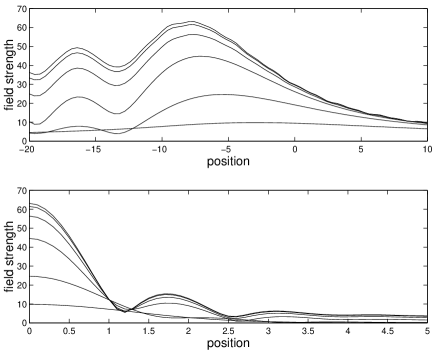
FIG. 1.: (a) Field strength $|F_{+}|$ of strongly focused Gaussian beams on the $z$ axis as a function of $Z\equiv(z-z_{0})/\lambda$. Note that the maximum field strength of the incoming field $\vec{F}_{0}$ is 1. The lens is located at $z=0$ and is characterized by $f=100\lambda$, so that $z_{0}\approx 100\lambda$. The incoming Gaussian beam has increasing values of $z_{{\rm in}}/\lambda=1\times 10^{3},3\times 10^{3},1\times 10^{4}\ldots 3\times 10^{5}$, resp., for the bottom to top curves. This implies for the outgoing beam decreasing values of $z_{R}\approx 10\lambda,10\lambda/3,\lambda,\ldots\lambda/30$. (b) Field strength in the focal plane as a function of the transverse coordinate $\rho/\lambda$.

The plots of the transverse mode profiles show that beyond a certain point the width of the field no longer decreases with stronger focusing. One cannot focus down a laser field to below a certain limit, roughly about half a wavelength, with the ideal lens with lens factor (11), no matter how small $z_{R}$ becomes. Moreover, one notes the asymmetry of the outgoing beam around the focal plane, in contrast to a paraxial beam which is symmetric in its focal plane. Since there is no a priori symmetry under reflections in the focal plane, this fact should not be surprising.

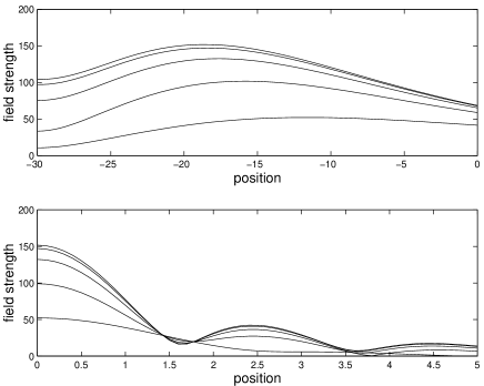
FIG. 2.: As Figure 1 but for $f=500\lambda$ and $z_{{\rm in}}/\lambda=3\times 10^{4},1\times 10^{5}\ldots 1\times 10^{6},3\times 10^{6}$.

Let us note here that strongly focused light beams in general will display phase singularities (rings in space where certain components of $\vec{E}$ vanish), of the kind investigated (both theoretically and experimentally) in Refs. [30, 31, 32, 33]. For Gaussian illumination of a spherical lens, however, no such singularities appear [31].

Finally, it may also be interesting to consider tightly focused donut beams, i.e., beams of light produced by focusing an incoming higher-order LG beam [17]. In the case of an incoming first-order LG beam, the incoming field distribution $\vec{F}_{0}$ can be written as (again assuming its focal plane coincides with the plane of the lens)

$$\vec{F}_{0}^{\pm}=\exp\left(-\frac{k\rho^{2}}{2z_{{\rm in}}}\right)\exp(\pm i\phi)\frac{\rho}{z_{{\rm in}}}\frac{\hat{x}+i\hat{y}}{\sqrt{2}}.$$ (34)

For the coefficients $\kappa^{\pm}_{\mu}$ we find then

$$\kappa^{\pm}_{\mu} = \delta_{m2,0}\pi k_{t}\frac{k_{z}+sk}{k}\int_{0}^{\infty}{\rm d}\rho\frac{\rho^{2}}{z_{{\rm in}}}J_{1}(k_{t}\rho)\times$$ (36)

$$\exp\left(-i\frac{k\rho^{2}}{2f}\right)\exp\left(-\frac{k\rho^{2}}{2z_{{\rm in}}}\right),$$

where $\delta_{m2,0}$ indicates that for the $+$ sign in (34) we get $\delta_{m2}$ and for the $-$ sign $\delta_{m0}$. These delta functions again express conservation of angular momentum: the outgoing beam possesses the same angular momentum as the incoming beam [26, 27], which has one unit of “spin” angular momentum and $\pm 1$ units of “orbital” angular momentum. The integral can be evaluated using

$$\int_{0}^{\infty}{\rm d}xx^{2}J_{1}(\beta x)\exp(-\alpha x^{2})=\frac{\beta}{4\alpha^{2}}\exp(-\beta^{2}/4\alpha),$$ (37)

and gives the result

$$\kappa_{\mu}=\pi\delta_{m2,0}\frac{k_{t}^{2}}{k^{2}}\frac{k_{z}+sk}{k}\frac{\xi^{2}}{z_{{\rm in}}}\exp\left(-\frac{k_{t}^{2}}{2k}\xi\right).$$ (38)

For $\kappa^{-}_{\mu}\propto\delta_{m0}$ there is a nonzero field on axis of a different polarization than the incoming field: the $z$ component, which would be neglected in the paraxial limit is in fact the only nonvanishing component on axis. In this case, however, the field on axis will be sensitive both to deviations of the lens from an ideal spherical lens, and to deviations of the incoming beam from a pure donut beam, even in the paraxial limit. For some explicit examples of this sensitivity see, for instance, Refs. [26, 32].

III Scattering light off of a single atom in free space

In this Section we will investigate the response of an atom located in the focal region of a strongly focused laser beam of the form (23) at $\vec{r}=\vec{r}_{0}$. We consider a $J_{g}=0\rightarrow J_{e}=1$ transition in the atom, as it is the simplest case where all three polarization components of the light in principle play a role. For simplicity we will assume the atom to be located on the $z$ axis, so that it in fact interacts only with a single ($\hat{\epsilon}_{+}$) polarization component; as mentioned above, the other two polarization components vanish on axis.

We are mostly interested in calculating the second-order correlation function for the light field as a function of position and time. For that purpose, the Heisenberg picture is the most convenient. In the Heisenberg picture, the electric field operator can be written as the sum of a “free” part and a “source” part [34],

$$\vec{E}=\vec{E}_{f}+\vec{E}_{s},$$ (39)

where the free part is given by

$$\vec{E}_{f}(\vec{r},t) = \sum_{\nu}\vec{F}_{\nu}(\vec{r})a_{\nu}\exp(-i\omega t)+h.c.$$ (40)

$$\equiv \vec{E}_{f}^{(+)}+\vec{E}_{f}^{(-)}.$$ (41)

Here we separated the field in positive- and negative-frequency parts and used the spatial mode functions $\vec{F}_{\nu}(\vec{r})$ from Eq. (5), with $a_{\nu}$ the annihilation operator for mode $\nu$. The source part for the case of a $J_{g}=0\rightarrow J_{e}=1$ transition is given by [34]

$$\vec{E}_{s}^{(+)}(\vec{r})=\sum_{i}\vec{\psi}_{i}(\vec{r}\prime)\sigma_{i}^{-}(t-|\vec{r}\prime|/c),$$ (42)

where $\vec{r}\prime=\vec{r}-\vec{r}_{0}$, and $\sigma_{i}^{-}$ is the atomic lowering operator, and the sum is over three independent polarization directions $i=\pm 1,0$. Equation (42) is valid in the far field, with $\vec{\psi}_{i}(\vec{r})$ the dipole field

$$\vec{\psi}_{i}(\vec{r})=\frac{\omega_{0}^{2}}{4\pi\varepsilon_{0}c^{2}}\left[\frac{\vec{d}_{i}}{r}-\frac{(\vec{d}_{i}\cdot\vec{r})\vec{r}}{r^{3}}\right].$$ (43)

Here $\omega_{0}$ is the atomic resonance frequency, and $\vec{d}_{i}=d\hat{u}_{i}$ is the dipole moment between the ground state $|g\rangle$ and the excited state $|e_{i}\rangle$ in terms of the standard unit circular vectors,

$$\hat{u}_{-1} = \hat{\epsilon}_{-},$$ (44)

$$\hat{u}_{0} = \hat{z},$$ (45)

$$\hat{u}_{1} = -\hat{\epsilon}_{+},$$ (46)

and the reduced atomic dipole matrix element $d$.

Expressions containing the electric field in time-ordered and normal-ordered form (as measured using standard photon detectors), such as the intensity and the second-order intensity correlation function, can be transformed into what Ref. [34] denotes as ${\cal O}$-ordered form, where $\vec{E}^{(+)}_{s}$ is placed to the left of $\vec{E}^{(+)}_{f}$, $\vec{E}^{(-)}_{f}$ to the left of $\vec{E}^{(-)}_{s}$, and where the source parts are time-ordered. For instance, if we assume the initial state of the light field to be a coherent state then the normally ordered intensity can be written as

$$I(t,\vec{r}) = \langle\vec{E}^{(-)}(t,\vec{r})\cdot\vec{E}^{(+)}(t,\vec{r})\rangle$$ (47)

$$= \sum_{i,j=-1,0,1}\vec{\psi}_{j}^{*}(\vec{r})\cdot\vec{\psi}_{i}(\vec{r})\sigma_{ee}^{ij}(t_{r})+|\alpha|^{2}|\vec{F}_{{\rm out}}(\vec{r})|^{2}$$ (49)

$$+\sum_{i=-1,0,1}2{\rm Re}[\alpha^{*}\exp(i\omega_{0}t)\vec{F}_{{\rm out}}^{*}(\vec{r})\cdot\vec{\psi}_{i}(\vec{r})\sigma_{eg}^{i}(t_{r})],$$

where $\alpha$ determines the amplitude of the coherent state, such that $\langle\vec{E}^{(+)}\rangle=\alpha\vec{F}_{{\rm out}}$. In Eq. (47) we introduced the retarded time $t_{r}=t-|\vec{r}^{\prime}|/c$, and $\sigma_{eg}^{i}=\langle\sigma_{i}^{-}\rangle$ and $\sigma_{ee}^{ij}=\langle\sigma_{i}^{+}\sigma_{j}^{-}\rangle$ are expectation values of the corresponding atomic operators. The three terms in (47) correspond to the intensity $I_{d}$ of the dipole field, $I_{L}$ of the incoming laser beam, and the interference term. Similarly, the second-order correlation function (where we now suppress the dependence of the fields on $\vec{r}$)

$$G^{(2)}(t,\tau,\vec{r})=$$ (51)

$$\sum_{l,m=x,y,z}\langle E_{l}^{(-)}(t)E_{m}^{(-)}(t+\tau)E_{m}^{(+)}(t+\tau)E_{l}^{(-)}(t)\rangle$$ (52)

consists of 16 terms. For $\tau=0$, 7 of those vanish identically, and the remaining ones are

$$G^{(2)}(t,0,\vec{r})=|\alpha|^{4}|\vec{F}_{{\rm out}}|^{4}+\sum_{i,j}2|\alpha|^{2}|\vec{F}_{{\rm out}}|^{2}\vec{\psi}^{*}_{i}\cdot\vec{\psi}_{j}\sigma_{ee}^{ij}(t_{r})$$ (53)

$$+\sum_{i}4{\rm Re}(\alpha^{*}\exp(i\omega_{0}t))\vec{F}^{*}_{{\rm out}}\cdot\vec{\psi}_{i}|\alpha|^{2}|\vec{F}_{{\rm out}}|^{2}\sigma^{i}_{eg}(t_{r}))$$ (54)

$$+\sum_{i,j}2|\alpha|^{2}(\vec{F}_{{\rm out}}\cdot\vec{\psi}^{*}_{i})(\vec{F}_{{\rm out}}^{*}\cdot\vec{\psi}_{j}\sigma_{ee}^{ij}(t_{r})).$$ (55)

For the evaluation of the atomic quantities we assume the atom reaches a steady state. Define $C_{i}=\alpha\vec{d}_{i}^{*}\cdot\vec{F}_{{\rm out}}(0)/\hbar$ and the matrices ${\cal M}$ and ${\cal M}_{1,2}$ by

$${\cal M}_{1}^{ij} = \frac{C_{i}C_{j}^{*}/\Gamma}{\Gamma/2+i\Delta}$$ (56)

$${\cal M}_{2}^{ij} = \frac{C_{i}C_{j}^{*}/\Gamma}{\Gamma/2-i\Delta}$$ (57)

$${\cal M} = ({\cal M}_{1}+{\cal M}_{2})/({\cal M}_{1}+{\cal M}_{2}+\openone)$$ (58)

with $\Gamma$ the decay rate of the excited states [34],

$$\Gamma=\frac{d^{2}\omega_{a}^{3}}{3\pi\hbar\epsilon_{0}c^{3}}$$ (59)

and $\Delta=\omega_{0}-\omega_{a}$ the detuning of the laser field from atomic resonance. In the steady state we have then

$$\sigma_{gg} = \frac{1}{1+{\rm Tr}{\cal M}},$$ (60)

$$\sigma_{ee} = \sigma_{gg}{\cal M},$$ (61)

$$\sigma_{eg} = \frac{i\sigma_{gg}\vec{C}-i\sigma_{ee}\vec{C}}{\Gamma/2-i\Delta}\exp(-i\omega_{0}t).$$ (62)

We are mainly interested in finding the maximum effect the atom may have on the outgoing beam. We therefore consider the case of weak on-resonance excitation, i.e., $|\vec{C}|\ll\Gamma$ and $\Delta=0$. We then calculate $g^{(2)}(\tau,\vec{r})\equiv G^{(2)}(\tau,\vec{r})/I^{2}(\vec{r})$ at $\tau=0$—there is no dependence on $t$ in the steady state and for simplicity we leave the argument $t$ out— as a function of position in the far field. Results are shown in Figures 3–4. The distance to the atom is fixed at $R=50\lambda$ for numerical reasons. Note that the angular spectrum does depend on the precise value of $R$. Only in the forward direction do the dipole field and a laser field display the same asymptotic behavior. In the forward direction, i.e. on the $z$ axis, the laser field turns out to overwhelm the scattered field, irrespective of how strongly the light is focused onto the atom. This may be compared to a similar result for classical scattering from spherical dielectrics with light focused down to spot sizes larger than 5 times the size of the spheres [35]. Hence we find that $g^{(2)}(0,\vec{r})\approx 1$ for forward scattering, which is in sharp contrast with the result from [18] which predicts a large bunching effect (i.e., $g^{(2)}\gg 1$) for tight focusing. The figure also shows that in a perpendicular direction the dipole field dominates, so that $g^{(2)}(0,\vec{r})=0$ for $\phi\rightarrow\pi/2$ (i.e., there the light is almost purely fluorescence light, which is anti-bunched [36, 37]). $g^{(2)}$ reaches a maximum around angles where the scattered and laser fields are comparable in magnitude. The oscillations indicate that $g^{(2)}(0,\vec{r})$ is very sensitive to the relative phase between the dipole and the laser field. In fact, maxima in $g^{(2)}$ appear when the free field and the dipole field interfere destructively. Indeed, this implies that the total field is smaller than the laser field, which implies a photon has just been absorbed by the atom. The atom is therefore in its excited state, and hence one can expect a fluorescent photon to appear soon, thus leading to a strong bunching effect.

Going from Fig. 3 to 4 corresponds to tighter focusing ($z_{R}$ decreases by a factor of 2) and we see that

1. In the forward direction the ratio of the amounts of laser and scattered light decreases (but it’s still much larger than 1).

2. The region where $g^{(2)}$ reaches its maximum moves outward to larger angles $\phi$.

3. The ratio of the amounts of laser and scattered light at $\phi=90^{o}$ increases by a large amount.

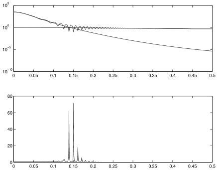
FIG. 3.: Plot (a) gives the relative intensities of the laser field, the dipole field and the total field as a function of the angle $\phi/\pi$ with the $z$ axis (i.e, at position $\vec{r}=[R\sin\phi,0,R\cos\phi]$ where we chose $R=50\lambda$ here and for all further calculations. The parameters for the incoming beam and the lens are $f=500\lambda$ and $z_{{\rm in}}=3\times 10^{4}\lambda$, so that $z_{R}=8.3\lambda$ and $z_{0}=500\lambda$, where we chose $\lambda=852$nm, corresponding to the D2 transition in Cs, and the atomic dipole moment $d$ adjusted so as to give the correct corresponding spontaneous emission rate $\Gamma=2\pi\times 2.6$MHz for the 6$P_{3/2}$ states of Cs. Plot (b) gives $g^{(2)}(0,\vec{r})$ as a function of $\phi/\pi$.

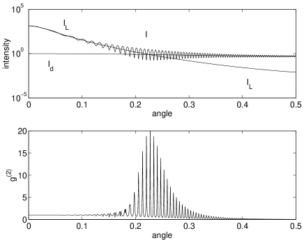
FIG. 4.: As Figure 3, but the parameters for the incoming beam and the lens are $f=500\lambda$ and $z_{{\rm in}}=6\times 10^{4}\lambda$, so that $z_{R}=4.2\lambda$ and $z_{0}=500\lambda$.

We can compare these results with those for a Gaussian beam with the same beam parameters. Figures 5 and 6 show that the 3 conclusions still hold. However, a Gaussian beam exaggerates the amount of light in the forward direction (small $\phi$) at the cost of greatly underestimating it for larger angles. This implies that the region where $g^{(2)}$ reaches its maximum is moved to smaller angles $\phi$ for a paraxial beam.

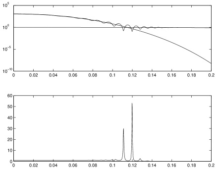
FIG. 5.: As Figure 3, but for a paraxial beam characterized by the same beam parameters $z_{R}=8.3\lambda$ and $z_{0}=500\lambda$.

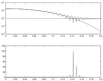
FIG. 6.: As Figure 4, but for a paraxial beam characterized by the same beam parameters $z_{R}=4.2\lambda$ and $z_{0}=500\lambda$.

We now focus on forward scattering, and plot in Figure 7 the ratio of the intensities of the laser field and the dipole field, i.e., $K=|\vec{E}_{f}|^{2}/|\vec{E}_{s}|^{2}$, in the forward direction ($\phi=0$) as a function of the normalized (dimensionless) beam width $w$, defined as

$$w=\sqrt{\frac{z_{R}}{\pi\lambda}}.$$ (63)

The laser field intensity is seen to be much larger than the dipole field intensity, by at least a factor of $\sim 500$. For a Gaussian beam, on the other hand, the ratio becomes arbitrarily small for small $w$. This has immediate consequences for the value of $g^{(2)}(0,\vec{r})$ (see Figure 8).

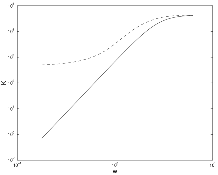
FIG. 7.: The relative intensity of the laser beam to the dipole field in the forward direction, $K$, as a function of the beam width parameter $w$ for the case $f=500\lambda$. Since $z_{R}\leq f/2$, the beam width $w$ satisfies $w\leq 6.3$. The dashed curve corresponds to the exact solution, the solid curve to a Gaussian beam.

For a Gaussian beam, the intensity in the focal region is not bounded. In fact, for decreasing values of $w$, more and more energy is concentrated in the focal region, so much so that the dipole field will eventually dominate the field in the forward direction. In that case, the forward direction will display anti-bunching (for $w$ smaller than approximately 0.07). Before that, however, $g^{(2)}$ reaches a large maximum at about $w\approx 0.2$, namely when the dipole and laser fields are comparable in magnitude. For larger values of $w$, the scattered field will be negligible, and $g^{(2)}\rightarrow 1$, but only after reaching a minimum close to zero around $w=0.3$. The latter characteristics were also found in Ref. [18]. For the exact solutions, however, none of these effects is present, and the laser field always dominates the dipole field, so that $g^{(2)}\approx 1$ for all values of the beam width.

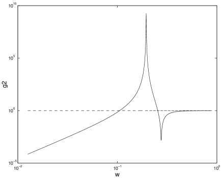
FIG. 8.: $g^{(2)}(0,\vec{r}))$ in the forward direction as a function of the beam width parameter $w$. The solid curve corresponds to a Gaussian beam, the dashed curve to the exact solution (23).

Let us finally quantify the effects of focused light on atoms in a different way by considering the following. If the atomic dipole is $\vec{d}$, then the relevant quantity determining the excitation probability of an atom is $|\vec{d}\cdot\vec{E}^{(-)}(\vec{r}_{0})|^{2}$ evaluated at the atom’s position $\vec{r}_{0}$, while the total incoming energy flux is given by $\int{\rm d}S|\vec{E}^{(-)}|^{2}$. In contrast to the naive expectation $R\sim\sigma/A$, the actual ratio $R_{s}$ that determines the fraction of the energy incident on the atom which will be scattered is given by

$$R_{s}=\frac{3\lambda^{2}|\hat{d}\cdot\vec{E}^{(-)}(\vec{r}_{0})|^{2}}{2\pi\int{\rm d}S|\vec{E}^{(-)}|^{2}}.$$ (64)

This ratio is plotted in Fig. 9 as a function of the width $w=w_{R}/\lambda$ for several values of the focal parameter $f$. For smaller $f$ the best achievable ratio increases, as expected, but for realistic lens parameters, the optimum $R_{s}$ is about 20%. Even for small values of $f$, the maximum scattering ratio does not go beyond 1/2. This can be understood by noting that the optimum shape of the illuminating field would be a dipole field. Here with light coming only from one direction, one may expect $R_{s}$ to be at most 1/2. Obviously, with one mirror behind the atom, one can improve the scattering ratio $R_{s}$ by a factor of 2. And of course, by building an optical cavity around the atom the atom-light interaction can be enhanced by many orders of magnitude, but that’s a different story [39].

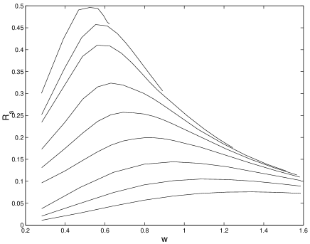
FIG. 9.: The scattering ratio $R_{s}$ as a function of the normalized beam width $w=w_{R}/\lambda$. The different curves correspond to $f/\lambda=2.5,5,10,25,50,100,250,500,1000$ resp., for top to bottom curves.

IV Discussion and conclusions

We constructed propagating wave solutions of Maxwell’s equations describing tightly focused laser beams. The method we used consisted of expanding the outgoing beam in a complete set of solutions and matching it at the plane of a lens to a given incoming beam. The lens was assumed ideal (infinitely thin) and the incoming beam was chosen to be Gaussian.

We then investigated quantum-statistical properties of the light emitted by an atom in free space, when it is illuminated by such a beam. Light detected in the forward direction does not display any bunching, nor anti-bunching effects: the field is dominated by the laser light, and the normalized second-order intensity correlation function is practically unity. This may not be surprising but is in contrast to results obtained by using Gaussian beams and by a standard quantum-optical input-output model. Gaussian beams are no longer valid approximate solutions under strong focusing conditions, and in particular exaggerate the focal intensity by a large amount. On the other hand, the input-output formalism implicitly assumes that the scattered field propagates in the same manner as the incident light beam: in free space this would correspond to illumination with a laser field whose profile mimics the dipole pattern. Inside a cavity, however, the model is expected to apply, as the situation there is to a good approximation one-dimensional. Indeed, the equations ultimately assume the same form as those for an atom coupled to a cavity mode in the bad-cavity limit [38].

Although the model of a single ideal lens with a simple lens factor of Eq. (11) may not lead to the strongest possible focusing [15], the amount of focusing reached is sufficiently strong (focusing areas $A$ less than or equal to the absorption cross section $\sigma=3\lambda^{2}/(2\pi)$ of an atom) to conclude that the interaction a focused light beam with an atom is not as strong as might be expected on the basis of the ratio $\sigma/A$ (see Fig. 9). Its consequence for quantum information processing may be phrased as: in free space it is easier and more efficient to use light to process quantum information carried by an atom, than to use an atom to process quantum information carried by photons.

REFERENCES

- [1] J.I. Cirac and P. Zoller, Phys. Rev. Lett. 78, 3221 (1995).
- [2] D.J. Wineland, C. Monroe, W.M. Itano, D. Leibfried, B.E. King, and D.M. Meekhof, J. Res. Natl. Inst. Stand. Technol. 103, 259 (1998).
- [3] A. Steane, Rep. Progr. Phys. 61, 117 (1998).
- [4] H.C. Nägerl, D. Leibfried, H. Rohde, G. Thalhammer, J. Eschner, F. Schmidt-Kaler, and R. Blatt, Phys. Rev. A 60, 145 (1999).
- [5] J.I. Cirac, P. Zoller, H.J. Kimble and H. Mabuchi, Phys. Rev. Lett. 78, 3221 (1997).
- [6] S.J. van Enk, J.I. Cirac and P. Zoller, Phys. Rev. Lett. 78, 4293 (1997); Science 279, 205 (1998).
- [7] S.L. Braunstein, C.M. Savage, and D.F. Walls, Opt. Lett. 15, 628 (1990).
- [8] Q.A. Turchette, C.J. Hood, W. Lange, H. Mabuchi and H.J. Kimble, Phys. Rev. Lett. 75, 4710 (1995).
- [9] J.D. Jackson, Classical Electrodynamics (Wiley, New York, 1999).
- [10] B.W. Peuse, M.G. Prentiss, and S. Ezekiel, Phys. Rev. Lett. 74, 269 (1982).
- [11] D.J. Wineland, W.M. Itano and J.C. Bergquist, Opt. Lett. 12, 389 (1987).
- [12] W.E. Moerner and T. Baschè, Angew. Chem. Int. Ed. Engl. 32, 457 (1993) and references therein.
- [13] W.E. Moerner and M. Orrit, Science, 283, 1670 (1999).
- [14] L. Fleury, J.-M. Segura, G. Zumofen, B. Hecht, and U.P. Wild, Phys. Rev. Lett. 84, 1148 (2000).
- [15] Ph. Grangier, private communication.
- [16] S.J. van Enk and H.J. Kimble, Phys. Rev. A 61, 051802(R) (2000).
- [17] A.E. Siegman, Lasers (University Science Book, Mill Valley, 1986).
- [18] H.J. Carmichael, Phys. Rev. Lett. 70, 2273 (1993).
- [19] P. Kochan and H.J. Carmichael, Phys. Rev. A 50, 1700 (1994).
- [20] Of course, at this point the electromagnetic field is just a classical solution of the Maxwell equations and reference to photons and is not necessary: we could have defined energy density, momentum density etc. instead.
- [21] S.J. van Enk and G. Nienhuis, J. Mod. Optics 41, 963 (1994); Europhys. Lett. 25, 497 (1994).
- [22] L. Allen, M.J. Padgett, and M. Babiker, Prog. Optics 39, 291 (1999).
- [23] M. Born and E. Wolf, Principles of Optics (Pergamon, New York, 1975).
- [24] J.W. Goodman, Introduction to Fourier Optics (Van Nostrand, New York, 1968).
- [25] For recent developments on the limits of focusing light see, e.g., T.R.M. Sales, Phys. Rev. Lett. 81, 3844 (1998).
- [26] S.J. van Enk and G. Nienhuis, Opt. Commun. 94, 147 (1992).
- [27] M. Beijersbergen, L. Allen, H.E.L.O. van Veen and J.P. Woerdman, Opt. Commun. 96, 123 (1996).
- [28] S.M. Barnett and L. Allen, Opt. Commun. 110, 670 (1994).
- [29] S.J. van Enk, Quantum Optics 6, 445 (1994).
- [30] M.W. Beijersbergen, Phase singularities in optical beams, Ph.D. Thesis, University of Leiden, The Netherlands (1996).
- [31] G.P. Karman, M.W. Beijersbergen, A. van Duijl, D. Bouwmeester, and J.P. Woerdman, J. Opt. Soc. Am. A 15, 884 (1998).
- [32] G.P. Karman and J.P. Woerdman, J. Opt. Soc. Am. A 15, 2862 (1998).
- [33] M.V. Berry, J. Mod. Optics 45, 1845 (1998).
- [34] W. Vogel and D.-G Welsch, Lectures on Quantum Optics, Akademie Verlag GmbH, Berlin (1994).
- [35] J.T. Hodges et al., Appl. Optics 34, 2120 (1995).
- [36] H.J. Carmichael and D.F. Walls, J. Phys. B 9, L43 (1976).
- [37] H.J. Kimble and L. Mandel, Phys. Rev. A 13, 2123 (1976).
- [38] P.R. Rice and H.J. Carmichael, IEEE J. Quant. Electron. 24, 1351 (1988).
- [39] Cavity Quantum Electrodynamics, Adv. At. Mol. Opt. Physics, Suppl. 2, Ed. P.R. Berman (Academic Press, Boston, 1994).