Adiabatic Elimination in Compound Quantum Systems with Feedback

Abstract

Feedback in compound quantum systems is effected by using the output from one sub-system (“the system”) to control the evolution of a second sub-system (“the ancilla”) which is reversibly coupled to the system. In the limit where the ancilla responds to fluctuations on a much shorter time scale than does the system, we show that it can be adiabatically eliminated, yielding a master equation for the system alone. This is very significant as it decreases the necessary basis size for numerical simulation and allows the effect of the ancilla to be understood more easily. We consider two types of ancilla: a two-level ancilla (e.g. a two-level atom) and an infinite-level ancilla (e.g. an optical mode). For each, we consider two forms of feedback: coherent (for which a quantum mechanical description of the feedback loop is required) and incoherent (for which a classical description is sufficient). We test the master equations we obtain using numerical simulation of the full dynamics of the compound system. For the system (a parametric oscillator) and feedback (intensity-dependent detuning) we choose, good agreement is found in the limit of heavy damping of the ancilla. We discuss the relation of our work to previous work on feedback in compound quantum systems, and also to previous work on adiabatic elimination in general.

I Introduction

The quantum theory of continuous Markovian feedback is now well understood [1, 2, 3, 4]. Continuous feedback arises in a situation where a system continuously interacts with its environment, and the environment is deliberately engineered such that the influence of the system on the environment acts back on the system at a later time. This can be described as a Markovian process when (a) the natural coupling of the system to the environment is approximately Markovian, and (b) the effective time-delay in the feedback process is negligible compared to any relevant time scale of the system. If the Markovian approximation is appropriate, this leads to the great simplification that the system evolution may be described by a master equation of the Lindblad form [5].

It is possible to divide quantum feedback into two categories, which we may call coherent and incoherent, following Lloyd [6] (but without being limited by his definitions). In the latter case of incoherent feedback, it is not necessary to use a quantum description of the entire feedback loop. Rather, at some point, it is permissible to change from a quantum to a classical description by invoking a measurement step. In a quantum optical context, this corresponds to electro-optical feedback [4] where a photocurrent derived from detecting the light radiated by the system is used to control electro-optical devices which change the behavior of the system. In the former case of coherent feedback, a quantum description of the entire feedback loop is necessary. In a quantum optical context this corresponds to all-optical feedback [4] in which the light radiated by the system is reflected so that in interacts with the system again, perhaps via some other system.

Continuous quantum feedback may be non-Markovian for a number of reasons. The coupling to the environment may be non-Markovian. The time delay in the feedback loop may be non-negligible. The feedback may act via a second system, the ancilla. In this paper we are concerned with the last possibility. This is of interest because it arises very naturally in quantum optics in both all-optical [4] and electro-optical [7] contexts. In principle, this sort of feedback can be described as a Markovian process in the larger state space of the system plus ancilla. In practice, this procedure is often not useful, because of the critical word larger in the previous sentence. If the required basis size of the system and ancilla are $N$ and $M$ respectively, then the Liouvillian for the compound system has of order $N^{4}M^{4}$ elements. Clearly for $M$ large, this is much larger than a Liouvillian for the system alone.

Consequently it would be an advantage to obtain a master equation for the system alone, without the ancilla. This is possible if the ancilla can be adiabatically eliminated. That is, if the ancilla has a decay rate much faster than any relevant system rate, so that it is always in a steady state determined by the system state. It is the purpose of this paper to determine numerically the conditions under which this is possible, and to derive the resultant master equations under those conditions, for a variety of general feedback systems.

Previous work in this area has left the situation somewhat confused. Wiseman and Milburn [4] considered all-optical feedback via an ancilla system, and adiabatically eliminated the ancilla. This was shown to be equivalent to electro-optical feedback for quadrature feedback. However, for intensity feedback it was the same only to second order in the feedback strength. Moreover, the master equation derived (to second order) was not of the Lindblad form.

Slosser and Milburn [7] considered electro-optic feedback of the photocurrent from the idler mode of a non-degenerate parametric oscillator onto the pump mode. Here the signal and idler mode formed the system and the pump mode was the ancilla. The procedure they adopted for deriving a master equation for the system was as follows. They expanded the feedback master equation for the compound system to first order in the feedback strength, adiabatically eliminated the pump mode, but the final result presented for the system master equation contained first and second order terms. As in Ref. [4], this second-order master equation was not of the Lindblad form. Furthermore, the steady-state field averages were calculated using an unstated all-order master equation (which was of the Lindblad form). There are other problems with this paper [8], but they are not relevant to the present work.

In this work we show how adiabatic elimination can be done rigorously in compound quantum feedback systems such as those of Refs. [4, 7]. As well as being of interest in the field of quantum feedback, the methods we use for adiabatic elimination are of more general interest. While adiabatic elimination of an ancilla mode which is linearly coupled to the system is well understood, adiabatic elimination with a nonlinear (e.g. proportional to the intensity) coupling is not. In particular, the methods we use here put the results obtained by Doherty and co-workers [10] on the motion of an atom coupled to a damped optical cavity mode on a more rigorous footing.

This paper is organized as follows. In Sec. II we consider simple direct-detection feedback, and the four types of analogous feedback in compound systems: electro-optic feedback via a two-level atom, electro-optic feedback via an optical mode, all-optical feedback via a two-level atom, and all-optical feedback via a mode. We show that in all four cases it is possible to eliminate the ancilla under suitable conditions, giving a master equation for the system alone. In Sec. III we compare the stationary state of these master equations with the solution of the full dynamics of the compound systems. For this test we choose the free dynamics of the system to be that of a below-threshold parametric oscillator, the quantity being fed back to be the intensity, and the quantity being controlled by the feedback to be the detuning. We also compare the results of all five feedback mechanisms with that caused by an analogous “reversible feedback” generated by a $\chi^{(3)}$ nonlinearity. In Sec. IV we conclude with a discussion of our results, and present a generalization of the all-optical case to multiple optical modes.

II Adiabatic Elimination

A Simple Feedback

In order to discern how the dynamics of a system are affected by a feedback loop that includes an ancilla, it is useful to know the master equation for simple feedback. By simple feedback it is meant that the measurement results, based on continuous observation of a source system, are immediately used to alter the evolution of the source without the involvement of any other quantum system. To use an example from quantum optics, a photodetector may register photon arrivals from a cavity at discrete times and, at these times, some specified change to the system may be made (see Fig. 1). Types of changes include altering the optical path length or damping rate of the cavity. In the remainder of this paper we will often use quantum optics terminology, but it should be remembered that the theory is not restricted to optical physics.

The most general form of the simple feedback master equation has been derived by Wiseman [3]. Consider a system with Hamiltonian $H$ and some dissipation at rate $\gamma$ and with lowering operator $c$. With $\hbar$ set equal to unity, the master equation is

$$\dot{\rho}(t)=-i[H,\rho]+\gamma{\cal D}[c]\rho,$$ (1)

where the Lindblad [5] superoperator is

$${\cal D}[c]={\cal J}[c]-{\cal A}[c],$$ (2)

where for arbitrary operators $A$ and $B$,

$${\cal J}[A]B=ABA^{\dagger}\;;\;\;{\cal A}[A]B=\mbox{$\frac{1}{2}$}\{A^{\dagger}A,B\}.$$ (3)

It is the dissipation which allows for continuous observation, the result of which is a current $I(t)$. In this paper we are concerned with what is known as direct detection where

$$I(t)=dN(t)/dt,$$ (4)

where $dN(t)$ is the point process (the increment in the number of photons counted) defined by

$$[dN(t)]^{2} = dN(t)$$ (5)

$${\rm E}[dN(t)] = \gamma dt{\rm Tr}[c^{\dagger}c\rho_{\rm c}(t)]$$ (6)

Here E denotes a classically probabilistic expectation value, while the c subscript denotes that the state $\rho_{c}$ is conditioned on the previous measurement results. We have assumed that the detection is perfectly efficient; the generalization to inefficient detectors is trivial [3].

Simple feedback arises from adding a Hamiltonian to the system evolution of the form

$$H_{\rm fb}(t)=I(t)Z$$ (7)

where $Z$ is an Hermitian system operator. Taking into account the singularity of $I(t)$, and the fact that the feedback must act after the measurement, it is possible to derive a master equation for the system with feedback, averaging over all realizations of the stochastic measurement record $I(t)$. The result is

$$\dot{\rho}=-i[H,\rho]+\gamma{\cal D}[e^{-iZ}c]\rho.$$ (8)

To compare this master equation with those obtained later it is useful to expand the exponentials to third order

$$\dot{\rho} \simeq {\cal C}[H]\rho+\gamma{\cal D}[c]\rho$$ (10)

$$+\;\gamma\left\{{\cal C}[Z]+\frac{1}{2}\left({\cal C}[Z]\right)^{2}+\frac{1}{6}\left({\cal C}[Z]\right)^{3}\right\}{\cal J}[c]\rho,$$

where ${\cal C}[A]B=-i[A,B]$ for arbitrary operators $A$ and $B$.

The derivation outlined above for the feedback master equation treats the photocurrent $I(t)$ as a classical stochastic process, which causes the conditioned system state $\rho_{\rm c}$ to undergo stochastic evolution (known as a quantum trajectory [11]). There is an alternative derivation which treats the photocurrent $I(t)$ as an operator. This derivation works in the Heisenberg picture, where the system evolution is described by stochastic operator differential equations known as quantum Langevin equations [12]. This method is useful for adiabatic elimination, so we will briefly review its features.

Quantum Langevin equations (QLE) are constructed without using the concept of measurement. The dissipative evolution of Eq. (1) can be derived in a quantum optical context from a linear coupling (in a rotating frame and with the rotating wave approximation)

$$V=i\sqrt{\gamma}[v^{\dagger}(t)c-c^{\dagger}v(t)]$$ (11)

between the system and a bath of harmonic oscillators. Here $v(t)$ is the bath annihilation operator at the point at which it interacts with the system. Just before this point, the bath is an input vacuum, with field operator $v_{\rm in}(t)$ satisfying [12]

$$[v_{\rm in}(t),v^{\dagger}_{\rm in}(t^{\prime})]=\delta(t-t^{\prime}),$$ (12)

and all normally-ordered moments vanishing. Just after this point, the bath is an output (non-vacuum) with field operator [12]

$$v_{\rm out}(t)=v_{\rm in}(t)+\sqrt{\gamma}c(t).$$ (13)

The photocurrent operator $I(t)$ is simply the intensity of the output field

$$I(t)=v_{\rm out}^{\dagger}(t)v_{\rm out}(t).$$ (14)

Adding together the evolution due to $H$, $V$, and $H_{\rm fb}$, and again noting that the feedback must act after the interaction, one can derive the following quantum Langevin equation for an arbitrary system operator $s$ [3]

$$ds = [v_{{\rm in}}^{{\dagger}}+\sqrt{\gamma}c^{{\dagger}}](e^{iZ}se^{-iZ}-s)[v_{{\rm in}}+\sqrt{\gamma}c]dt$$ (17)

$$+\gamma(c^{{\dagger}}sc-\frac{1}{2}sc^{{\dagger}}c-\frac{1}{2}c^{{\dagger}}cs)dt$$

$$-\sqrt{\gamma}[dV_{{\rm in}}^{{\dagger}}c-c^{{\dagger}}dV_{{\rm in}},s]+i[H,s]dt,$$

where $dV_{{\rm in}}=v_{{\rm in}}dt$. All operators have time argument $t$. When the expectation value of this equation is taken an equation is obtained that can be converted to the master equation (8) for simple feedback. If $Z$ is set to zero then the Langevin equation describes damping alone.

B Electro-optic Feedback via an Atom

The simplest possible ancilla system is a two-level atom (TLA). In this section we consider incoherent (electro-optic) feedback via this ancilla. The output from the system is monitored by direct detection, the results of which are used to affect the evolution of the two level atom which is coupled to the system, as shown in Fig. 2. The system and ancilla are assumed to have approximately the same resonant frequency. If the atom is to be adiabatically eliminated, it must be heavily damped, in which case it will mostly be in the ground state. Then the most natural form of feedback involves flipping the state of the TLA whenever the photodetector monitoring the system makes a detection. This can be achieved with a feedback Hamiltonian of the form

$$H_{{\rm fb}}=\frac{\pi}{2}\sigma_{x}I(t).$$ (18)

Here $\sigma_{x}$ is the usual Pauli spin matrix for describing an atomic state [13]. It could be realized experimentally by very briefly driving the atom with a pulse of on-resonance radiation (a ‘$\pi$’ pulse) which will flip it from the ground to the excited state.

With this form of feedback, the obvious coupling of the atom to the system to consider is one proportional to the excited state population operator $\sigma^{\dagger}\sigma$. Here $\sigma=(\sigma_{x}-i\sigma_{y})/2$ is the atomic lowering operator. Specifically,

$$H_{{\rm coupling}}=\sigma^{{\dagger}}\sigma K,$$ (19)

where $K$ is an arbitrary Hermitian system operator. When feedback onto the atom in the ground state occurs the upper state population jumps to a value of 1 and then decays away, due to coupling to the continuum of electromagnetic field modes. In other words, $\sigma^{\dagger}\sigma$ will tend to follow the photocurrent. Thus there is a strong similarity to simple feedback, if $K$ is chosen to be some scalar multiple of $Z$.

It is not hard to generalize Eq. (8) to include the TLA ancilla

$$\dot{W} = -i[H_{{\rm system}}+\sigma^{{\dagger}}\sigma K,W]$$ (21)

$$+{\cal D}[\exp(-i\frac{\pi}{2}\sigma_{x})c]W+\Gamma{\cal D}[\sigma]W,$$

where $\Gamma$ is the damping rate of the atom and $W$ is the density matrix for the compound system. The damping rate $\gamma$ of the system has been set equal to unity without loss of generality. Of course, the operators are now acting in the joint Hilbert space of the two systems so that $c\equiv c\otimes 1_{{\rm atom}}$ and $\sigma\equiv 1_{{\rm system}}\otimes\sigma$, etc.

The above master equation gives the evolution of the density operator for the compound system. At any time a partial trace of this operator over the atom could be performed to obtain the reduced density matrix for the system alone. However, in general, this cannot be done to the master equation itself in order to obtain a master equation for $\rho_{{\rm system}}(t)$. The obvious exception to this is the case where $K=0$ and the system is unaffected by the atom.

It is logical that a master equation for the system cannot be derived if the atom observables fluctuate, in response to the feedback, on the same time scale as the system observables. The effect of feedback would then depend on the constantly fluctuating state of the atom which, in turn, depends on previous feedback. Removing the atom operators from the master equation without removing information concerning the system is impossible due to the coupling that exists between them. Of course, a non-Markovian expression could be written down for the atom in terms of the system, but this would not lead to a Lindblad master equation without some further approximation.

If the atom reacts very quickly to the feedback and returns to its initial state before more feedback arrives (the next photodetection) then this well defined behavior can be built into a master equation for the system alone. In essence, the atom’s state is approximated by its equilibrium value with respect to the instantaneous state of the system and operators are replaced by their steady state expressions. This procedure is known as adiabatic elimination of the atom.

To proceed with the adiabatic elimination it is noted that the total density matrix can be expanded as

$$W= \rho_{0}\otimes|{\downarrow}\rangle\langle{\downarrow}|+\rho_{1}\otimes|{\downarrow}\rangle\langle{\uparrow}|$$ (22)

$$+\rho_{1}^{{\dagger}}\otimes|{\uparrow}\rangle\langle{\downarrow}|+\rho_{2}\otimes|{\uparrow}\rangle\langle{\uparrow}|,$$ (23)

where the $\rho$s exist in the system subspace. All possible states of the atom have been included ($|{\uparrow}\rangle$ and $\langle{\downarrow}|$ correspond to the excited and ground state respectively). This approach is particularly appropriate because of the small basis involved. If the above expression for $W$ is substituted into the master equation then the atom operators can act on the states of the atom. If the coefficients of the various orthogonal states are equated the following equations for the $\rho$s are obtained (the subscript ‘s’ indicates the system):

$$\dot{\rho_{0}} = {\cal C}[H_{\rm s}]\rho_{0}+{\cal J}[c]\rho_{2}-{\cal A}[c]\rho_{0}+\Gamma\rho_{2},$$ (24)

$$\dot{\rho_{1}} = {\cal C}[H_{\rm s}]\rho_{1}+i\rho_{1}K+{\cal J}[c]\rho^{{\dagger}}_{1}-{\cal A}[c]\rho_{1}-\frac{\Gamma}{2}\rho_{1},$$ (25)

$$\dot{\rho_{2}} = {\cal C}[H_{\rm s}]\rho_{2}+{\cal J}[c]\rho_{0}-{\cal A}[c]\rho_{2}-\Gamma\rho_{2}.$$ (26)

By tracing Eq. (23) over the atom the reduced density operator for the system is

$$\rho_{{\rm s}}=\rho_{0}+\rho_{2}$$ (27)

and its evolution equation is found to be

$$\dot{\rho}_{{\rm s}}=-i[H_{{\rm s}},\rho_{{\rm s}}]+{\cal D}[c]\rho_{{\rm s}}-i[K,\rho_{2}].$$ (28)

Without some approximation this is as far as the elimination of the atom can be taken. It is not a master equation due to the dependence upon $\rho_{2}$. As discussed previously, the limit in which the atom returns very quickly to the ground state after feedback needs to be considered. Because the probability for photodetection in any infinitesimal time period scales as the size of the period, the atom is in the ground state for almost all time. The approximation that $\rho_{{\rm s}}\approx\rho_{0}$ is therefore made. To obtain a master equation, an expression for $\rho_{2}$ in terms of $\rho_{0}$ is needed. From Eq. (26) it can be seen that if $\Gamma$ is large compared to the other co-efficients of $\rho_{2}$ (except possibly $K$) then fluctuations in this operator will be quickly damped out and $\dot{\rho_{2}}$ can then be set to zero. The effect of $K$ is to cause rotation of $\rho_{2}$ but not to affect its size. The physical picture already described is consistent with $\Gamma$ being large. Assuming $K\sim\Gamma\gg 1$ (where $K\sim\Gamma$ means that the operator $K$ scales like $\Gamma$), we find the steady state of $\rho_{2}$ to be

$$\rho_{2}=(\Gamma-{\cal C}[K])^{-1}{\cal J}[c]\rho_{0}.$$ (29)

When this is substituted into Eq. (28) the master equation for the system alone is obtained. With $Z=K/\Gamma$ it is

$$\dot{\rho}_{{\rm s}}=\{{\cal C}[H_{\rm s}]+{\cal D}[c]+{\cal C}[Z](1-{\cal C}[Z])^{-1}{\cal J}[c]\}\rho_{{\rm s}}.$$ (30)

It is not immediately clear that this master equation is of the Lindblad form [5]. However in appendix A 1 it is shown that it can be written as

$$\dot{\rho}_{{\rm s}}=-i[H_{{\rm s}},\rho_{{\rm s}}]+\int_{0}^{\infty}dqe^{-q}{\cal D}[e^{-iqZ}c]\rho_{{\rm s}}.$$ (31)

Some feeling for the nature of the master equation can be obtained by an expansion to third order in $Z$ (a small feedback approximation). This gives (subscripts dropped)

$$\dot{\rho} \simeq {\cal C}[H]\rho+{\cal D}[c]\rho$$ (33)

$$+\;\left\{{\cal C}[Z]+({\cal C}[Z])^{2}+({\cal C}[Z])^{3}\right\}{\cal J}[c]\rho.$$

These terms can be compared to the third order expansion of Eq. (10), with $\gamma=1$. The difference in second and higher order terms means that for large feedback the two systems will be significantly different.

C Electro-optic Feedback via a mode

The more challenging task of adiabatically eliminating an ancilla that has an infinite number of basis states is now considered. Optically, this could correspond to a single-mode cavity. The method of expanding the compound density matrix in terms of the lower number states of the ancilla is not appropriate due to the type of feedback that is utilized. Instead we use Quantum Langevin equations, which place no such restriction on the excitation of the ancilla.

The output field from the system is once again continuously monitored using direct detection (see Fig. 3). We take the feedback to be linear driving of the ancilla cavity. This causes a jump in amplitude of the ancilla cavity when there is a photodetection. It is described by the feedback Hamiltonian

$$H_{{\rm fb}}=\frac{\epsilon}{2}(-ib+ib^{{\dagger}})I(t),$$ (34)

where $b$ is the annihilation operator for the cavity, $\epsilon$ represents the amplitude of the coherent driving field and $I(t)$ is the operator for the photocurrent output from the system. Its effect can be determined from the Heisenberg equation of motion for $b$,

$$\dot{b}_{{\rm fb}}=-i[b,H_{{\rm fb}}]=\frac{\epsilon}{2}I(t).$$ (35)

Since $I(t)$ consists of $\delta$ functions, it is clear that the cavity field amplitude changes by an amount $\epsilon/2$ whenever a photodetection occurs. Note that here the implicit equation of motion for $b$ is sufficient to determine its evolution because the stochastic term is not dependent upon $b$ [14]. To provide a feedback circuit that is classically equivalent to simple feedback in the limit of large damping of the cavity, the following choice of coupling is made:

$$V=\frac{K}{2}(b+b^{{\dagger}}).$$ (36)

The equivalence can be seen if linear damping is included in Eq. (35). The slaved value of $b$ (in the limit of large damping $\dot{b}_{{\rm fb}}$ is set equal to zero) is then substituted into the coupling, which leaves it in the same form as a simple feedback Hamiltonian, given an appropriate choice of $K$.

The total master equation is

$$\dot{W} = -i[\frac{K}{2}(b+b^{{\dagger}})+H_{{\rm s}},W]$$ (38)

$$+{\cal D}[e^{\epsilon(-b+b^{{\dagger}})/2}c]W+\Gamma{\cal D}[b]W,$$

where once again $W$ is the density matrix describing the compound system and the damping of the system has been set equal to unity. The damping rate of the ancilla cavity is given by $\Gamma$. The quantum Langevin equation that corresponds to this master equation can be found by extending Eq. (17). The result for an arbitrary operator $r$ from either sub-system is

$$dr= v_{{\rm out}}^{{\dagger}}\left[e^{\epsilon(b-b^{{\dagger}})/2}re^{-\epsilon(b-b^{{\dagger}})/2}-r\right]v_{{\rm out}}dt$$ (42)

$$+{\cal D}[c^{{\dagger}}]rdt-[dV_{{\rm in}}^{{\dagger}}c-c^{{\dagger}}dV_{{\rm in}},r]$$

$$+\Gamma{\cal D}[b^{{\dagger}}]rdt-\sqrt{\Gamma}[dU_{{\rm in}}^{{\dagger}}b-b^{{\dagger}}dU_{{\rm in}},r]$$

$$+i[\frac{K}{2}(b+b^{{\dagger}})+H_{{\rm s}},r]dt,$$

where $dU_{{\rm in}}=u_{{\rm in}}dt$. The vacuum field input for the driven cavity, $u_{{\rm in}}$, has the same properties as $v_{{\rm in}}$.

To adiabatically eliminate the cavity, in the limit of heavy damping, a QLE will first be determined for a system operator, $s$. Eq. (42) is greatly simplified, as $s$ commutes with all driven cavity operators, to give

$$ds = {\cal D}[c^{{\dagger}}]sdt-[dV_{{\rm in}}^{{\dagger}}c-c^{{\dagger}}dV_{{\rm in}},s]$$ (44)

$$+i[\frac{K}{2}(b+b^{{\dagger}})+H_{{\rm s}},s]dt.$$

From this it is evident that an expression for $b$ is required if a master equation for the system alone is to be derived. The QLE for $b$ is

$$\dot{b}=-i\frac{K}{2}-\frac{\Gamma}{2}b-\sqrt{\Gamma}u_{{\rm in}}+\frac{\epsilon}{2}v_{{\rm out}}^{{\dagger}}v_{{\rm out}}.$$ (45)

For large $\Gamma$ the fluctuations in $b$ due to system operators will be quickly damped out. However, the stochastic terms have an infinite bandwidth, so that it is not strictly possible to slave an operator that only responds to a finite bandwidth, $\Gamma$, to these fluctuations. Although this problem can be side-stepped [4] it will prove advantageous to use the following equilibrium value of $b$

$$b = -\frac{iK}{\Gamma}-\int_{0}^{\infty}d\tau e^{-\Gamma\tau/2}\left[\sqrt{\Gamma}u_{{\rm in}}(t-\tau)\phantom{\frac{1}{2}}\right.$$ (47)

$$\phantom{-\frac{iK}{\Gamma}+\int_{0}^{\infty}d\tau}\left.-\;\frac{\epsilon}{2}v_{{\rm out}}^{{\dagger}}v_{{\rm out}}(t-\tau)\right].$$

The integral serves to determine the present contribution to $b$ from the stochastic terms at time $t-\tau$. This contribution falls off at rate $\Gamma/2$, the amplitude decay rate for the ancilla cavity. The term that is not under the integral comes from $K$ which is not stochastic and is therefore slowly varying compared to the highly damped cavity operators. Thus, $b$ can follow its evolution to a very good approximation.

To simplify matters the Langevin equation for $s$ will now be rearranged before substitution so that $u_{{\rm in}}$ will annihilate the vacuum when the expectation value is taken. This gives

$$ds = {\cal D}[c^{{\dagger}}]sdt-[dV_{{\rm in}}^{{\dagger}}c-c^{{\dagger}}dV_{{\rm in}},s]$$ (49)

$$+\,\frac{i}{2}\left(b^{{\dagger}}[K,s]+[K,s]b\right)dt+i[H_{{\rm s}},s]dt.$$

This is valid as $b$ and $b^{{\dagger}}$ commute with system operators. We cannot move the stochastic part $v_{\rm in}(t)$ of $v_{{\rm out}}(t-\tau)$ through the system commutator term to annihilate on the vacuum. However, it is possible to move the photocurrent itself at time $t-\tau$ as it commutes [12]. If the integrals that will annihilate on the vacuum when the trace over the bath is taken are ignored, then we are left with

$$\dot{s} = \frac{i\epsilon}{2}\left[K,s\right]\int_{0}^{\infty}d\tau e^{-\Gamma\tau/2}I(t-\tau)-\frac{1}{2\Gamma}\left[K,[K,s]\right]$$ (51)

$$+{\cal D}[c^{{\dagger}}]s-[v_{{\rm in}}^{{\dagger}}c-c^{{\dagger}}v_{{\rm in}},s]+i[H_{{\rm s}},s].$$

If the limit $\Gamma\rightarrow\infty$ is taken the integral reduces to $2I(t)/\Gamma$. The resultant equation for $\dot{s}$ is an implicit equation as it was derived by idealizing the properties of the cavity and environment [14]. An explicit equation is now required.

The term that needs to be treated in Eq. (51) can be written as

$$\dot{s}_{{\rm implicit}}=-\frac{\epsilon I{\cal C}[K]s}{\Gamma}.$$ (52)

This gives an explicit increment of the form [3, 15]

$$ds_{{\rm explicit}}=dN[\exp(-\epsilon{\cal C}[K]/\Gamma)-1]s,$$ (53)

where $dN=Idt=dN^{2}=v_{{\rm out}}^{{\dagger}}v_{{\rm out}}dt$. Remembering that the photocurrent is actually evaluated at a slightly earlier time than the system operators allows $v_{{\rm out}}$ to be moved to the right of the expression. If we put $Z=\epsilon K/\Gamma$, in order that our equations can be compared to simple feedback, then the total Langevin equation is

$$ds = [v_{{\rm in}}^{{\dagger}}+c^{{\dagger}}](e^{iZ}se^{-iZ}-s)[v_{{\rm in}}+c]dt$$ (56)

$$-\frac{\Gamma}{2\epsilon^{2}}\left[Z,[Z,s]\right]dt+{\cal D}[c^{{\dagger}}]sdt$$

$$-[dV_{{\rm in}}^{{\dagger}}c-c^{{\dagger}}dV_{{\rm in}},s]+i[H_{{\rm s}},s]dt.$$

When the expectation value is taken the stochastic part annihilates on the vacuum and the following master equation is obtained

$$\dot{\rho}=-i[H_{{\rm s}},\rho]+{\cal D}[e^{-iZ}c]\rho+\frac{\Gamma}{\epsilon^{2}}{\cal D}[Z]\rho.$$ (57)

The only difference from simple feedback is the third term. This is a term of second order in the feedback operator $Z$, and represents a type of noise that will tend to smooth over the interesting behavior of the system. Clearly it can be made arbitrarily small if $\epsilon$ is made large enough. A more detailed discussion of this term is given in Sec. III C

D All-optical Feedback via an atom

We turn now to coherent, or all-optical feedback. Once again we begin with the simplest possible ancilla, a two-level atom. All-optical feedback via an atom involves the reflection of the output field from the system onto the atom, where the atom is reversibly coupled to the system. Here, the resonant frequencies of the two systems are taken to be equal. It is different from electro-optic feedback as there is no measurement ste; the light is just reflected around a loop with the use of mirrors (see Fig. 4). The theoretical description of such systems was developed largely by Carmichael [16] and Gardiner [17] and has been termed Cascaded Open Systems theory. If linear bath-system couplings are assumed then the compound master equation is

$$\dot{W}= -i[H_{\rm s}+V,W]+{\cal D}[c]W+\Gamma{\cal D}[\sigma]W$$ (58)

$$+\sqrt{\Gamma}\left([cW,\sigma^{{\dagger}}]+[\sigma,Wc^{{\dagger}}]\right).$$ (59)

The system damping has been set equal to unity as usual and $\Gamma$ is the damping rate of the atom.

In order to investigate the degree to which all-optical feedback can replicate electro-optical simple feedback, a coupling is chosen that is linear in the excited state population of the atom. We expect this operator to follow the output photocurrent from the system. That is, we assume a coupling

$$V=K\sigma^{{\dagger}}\sigma$$ (60)

identical to that in Sec. II B. Making the expansion of Eq. (23) gives the following for the $\rho$s

$$\dot{\rho_{0}} = {\cal C}[H_{\rm s}]\rho_{0}+{\cal D}[c]\rho_{0}+\Gamma\rho_{2}+\sqrt{\Gamma}(c\rho_{1}+\rho_{1}c^{{\dagger}}),$$ (61)

$$\dot{\rho_{1}} = {\cal C}[H_{\rm s}]\rho_{1}+{\cal D}[c]\rho_{1}+\sqrt{\Gamma}(\rho_{2}-\rho_{0})c^{{\dagger}}$$ (63)

$$+\,i\rho_{1}K-\frac{\Gamma}{2}\rho_{1},$$

$$\dot{\rho_{2}} = {\cal C}[H_{\rm s}]\rho_{2}+{\cal D}[c]\rho_{2}-\sqrt{\Gamma}(c\rho_{1}+\rho_{1}c^{{\dagger}})$$ (65)

$$-\,i[K,\rho_{2}]-\Gamma\rho_{2}.$$

The above equations lead to an equation of motion for the system density operator of

$$\dot{\rho}={\cal C}[H_{\rm s}]\rho+{\cal D}[c]\rho-i[K,\rho_{2}],$$ (66)

which is the same as Eq. (28). To find an expression for $\rho_{2}$ the normal procedure of taking $\Gamma$ large compared to ${\cal C}[H_{\rm s}]$ is performed. Thus, $\rho_{1}$ can be slaved to system operators, $\rho_{0}$ and $\rho_{2}$. Now as we only require a master equation which gives the leading order effect in $\Gamma^{-1}$ of the ancilla on the system, $\rho_{2}$ can be set equal to zero in the $\rho_{1}$ equation, which is the approximation $\rho_{0}\approx\rho$. This is valid as $\rho_{2}\sim\rho_{0}/\Gamma$. By substituting the slaved expression for $\rho_{1}$ into that for $\rho_{2}$ we find after simplification

$$\rho_{2}=\frac{4}{\Gamma}{\cal J}\left[\left(1+\frac{2iK}{\Gamma}\right)^{-1}c\right]\rho_{0}.$$ (67)

This can now be substituted into Eq. (66) to obtain a master equation. Writing $Z=4K/\Gamma$, we have

$$\dot{\rho}={\cal C}[H_{\rm s}]\rho+{\cal D}[c]\rho+{\cal C}[Z]{\cal J}\left[\left(1+\frac{Zi}{2}\right)^{-1}c\right]\rho,$$ (68)

which is the same as the simple feedback Eq. (10) to second order. The third order term is

$$\frac{1}{4}{\cal C}[Z]({\cal J}[Z]-2{\cal A}[Z]){\cal J}[c]\rho.$$ (69)

Again it is not obvious that Eq. (68) is in the Lindblad form, but it is shown in Appendix A 2 that it can be written as

$$\dot{\rho}=-i[H_{{\rm s}},\rho]+{\cal D}\left[\exp\left(-2i\arctan{\frac{Z}{2}}\right)c\right]\rho.$$ (70)

E All-optical Feedback via a mode

The final compound system that will be considered involves the output field from a system being reflected onto an optical cavity that is coupled back to the system (see Fig. 5). A Faraday Isolator (comprised of a Faraday Rotator and a Polarization dependent Beam Splitter) prevents reflected light from the cavity returning to the system. The only difference in the total master equation from the previous section is the replacement of the atom lowering operator $\sigma$ with the annihilation operator $b$. Thus a coupling of the form $V=Kb^{{\dagger}}b$ is considered.

The derivation of a master equation for the system alone follows similar lines to that of Sec. II C. The QLE for an arbitrary operator is [17]

$$dr = +i[H_{{\rm s}}+V,r]dt+{\cal D}[c^{{\dagger}}]rdt-[dV_{{\rm in}}^{{\dagger}}c-c^{{\dagger}}dV_{{\rm in}},r]$$ (73)

$$+\Gamma{\cal D}[b^{{\dagger}}]rdt-\ \sqrt{\Gamma}[dV_{{\rm in}}^{{\dagger}}b-b^{{\dagger}}dV_{{\rm in}},r]$$

$$+\sqrt{\Gamma}(b^{{\dagger}}rc+c^{{\dagger}}rb-rb^{{\dagger}}c-c^{{\dagger}}br)dt.$$

For a system operator this becomes

$$ds = {\cal D}[c^{{\dagger}}]sdt-[dV_{{\rm in}}^{{\dagger}}c-c^{{\dagger}}dV_{{\rm in}},s]$$ (75)

$$+\,i[H_{{\rm s}}+Kb^{{\dagger}}b,s]dt.$$

The next step is to find an equation for $b$. The QLE that governs it is

$$db=-(\frac{\Gamma}{2}b+\sqrt{\Gamma}v_{{\rm in}}+\sqrt{\Gamma}c+iKb)dt.$$ (76)

This justifies our initial presumption that the cavity photon number would follow the photocurrent. For $\Gamma$ large it is possible to slave $b$ to the system operators and to form an integral expression for the contribution from the stochastic term, as in Sec. II C. The result is

$$b = -\frac{2}{\sqrt{\Gamma}}\left(1+\frac{2iK}{\Gamma}\right)^{-1}c$$ (78)

$$+\sqrt{\Gamma}\int_{0}^{\infty}d\tau e^{-\Gamma\tau(1+2iK/\Gamma)/2}v_{{\rm in}}(t-\tau).$$

The same trick of rearranging the QLE for the system operator is again used so that, in this case, all of the integral terms annihilate. We put

$$i[Kb^{{\dagger}}b,s]dt=ib^{{\dagger}}[K,s]bdt.$$ (79)

Substituting into this the expression for $b$ and $b^{{\dagger}}$ gives four terms, only one of which is non-zero when the trace over the bath is taken. This term is

$$\frac{4ic^{{\dagger}}}{\Gamma}\left(1-\frac{2iK}{\Gamma}\right)^{-1}\left[K,s\right]\left(1+\frac{2iK}{\Gamma}\right)^{-1}c.$$ (80)

In effect, an implicit equation has been derived that has no contribution from stochastic operators, resulting in there being no need for an implicit/explicit distinction. It is now possible to turn the equation for $ds$ into a master equation for the system. When this is done we arrive at the same result as Eq. (68). The conclusion is that to first order in $\Gamma^{-1}$, the cavity has the same effect on the system that the atom does, when included in an all-optical feedback loop.

In hindsight, this is what we should have expected, as in the limit of large damping only the lowest number states of the cavity will be occupied with significant probability. One could therefore have expanded the total density matrix analogously to the TLA system to obtain the same equations immediately.

The reason why electro-optic feedback onto an atom and a cavity were not equivalent is due to the more singular nature of the driving of the ancilla. When a detection on the system is made the field amplitude of the cavity jumps, leading to occupation of higher photon number states. These states are, therefore, essential to the description of the compound system. Electro-optic feedback onto the atom cannot replicate this behavior.

III COMPARISON WITH EXACT RESULTS

We have shown that in principle it is possible to consider a variety of different sorts of feedback in compound quantum systems, and to adiabatically eliminate the ancillary system to arrive at master equations for the system of interest alone. These master equations should be exact in the limit that the ancilla is damped infinitely faster than the system. In practice, this will never be the case, so it is an interesting question to find out under what conditions the equations are valid. This can be done by simulating the full master equation for the compound system and comparing to the results of the master equation for the system alone.

To make such a comparison requires specifying the feedback operator, $Z$, and the system Hamiltonian, $H_{{\rm s}}$. Once this is done, a comparison can be made by looking at the stationary solutions of the respective master equations. While this could be criticised as not being a complete test, it has the advantages of definiteness and ease of calculation (in some cases at least). Furthermore, we choose a system (a damped optical mode) and Hamiltonians $H_{\rm s}$ and $Z$ such that the stationary solutions have enough structure for the comparison to be interesting. The comparison is both quantitative and qualitative, with the use of the Bures distance [18] as a measure of the difference between the state matrices and the Wigner function [19] to illustrate them.

In the hope of getting some interesting states we take the system to be a damped single mode optical cavity. That is, we choose $c=a$, an annihilation operator satisfying $[a,a^{\dagger}]=1$. We choose a system Hamiltonian (in a rotating frame) of

$$H=-\frac{i\lambda}{4}\left[a^{2}-(a^{{\dagger}})^{2}\right],$$ (81)

This describes a degenerate parametric amplifier (“two photon” driving), which can be realized by driving an intracavity crystal with a $\chi^{(2)}$ non-linearity with light at twice the resonant frequency. For $\lambda$ positive, this results in squeezing of the $X_{2}$ quadrature of the field inside the cavity, and stretching of the $X_{1}$ quadrature. The two quadratures are defined in this paper as

$$X_{1} = a+a^{{\dagger}}$$ (82)

$$X_{2} = -i(a-a^{{\dagger}}).$$ (83)

Without feedback, the master equation with two-photon driving and damping will have a stationary solution only for $\lambda<1$. That is, $\lambda$ is the threshold parameter.

The feedback operator is chosen to be

$$Z=\chi a^{{\dagger}}a.$$ (84)

We can get a feel for the effect of this type of feedback by using $Z$ in the simple feedback Hamiltonian given in Eq. (7). That is,

$$H_{{\rm fb}}(t)=\chi I(t)a^{{\dagger}}a.$$ (85)

This represents a detuning of the system cavity proportional to the photocurrent. It will cause the master equation to have a stationary solution regardless of $\lambda$, as will be shown. As the mean photocurrent is equal to the expectation value of the photon number operator for the system, this Hamiltonian is akin to a $\chi^{(3)}$ Kerr non-linearity [19]. In Sec. III F a comparison of feedback to such a nonlinearity is made.

A Simple Feedback

The master equation for simple feedback is now

$$\dot{\rho}=-\frac{\lambda}{4}\left[a^{2}-(a^{{\dagger}})^{2},\rho\right]+{\cal D}[e^{-i\chi a^{{\dagger}}a}a]\rho.$$ (86)

To simplify the numerical analysis we choose a single feedback strength for which simulations will be run. To aid this decision the effect of feedback is analyzed. Consider the following quantity:

$${\cal J}\left[e^{-i\chi a^{{\dagger}}a}\right]\rho.$$ (87)

If this is evaluated in the number basis then we get

$$\langle{n}|{\cal J}\left[(e^{-i\chi})^{a^{{\dagger}}a}\right]\rho|{m}\rangle=(e^{-i\chi})^{n-m}\rho_{nm}.$$ (88)

Now this particular system has the property that $\rho_{nm}=0$ for $|n-m|$ odd as the two photon driving is the only source of coherences. These coherences exist between elements with $|n-m|$ even. Hence, if $\chi=q\pi$, with $q$ an integer, then the feedback has no effect. Investigation into the states produced with a value of feedback close to this revealed that they are extremely sensitive to any parameter variation. This implies that it is not a suitable regime for the testing of adiabatic elimination. The most obvious alternative is to choose the maximum feedback regime. It is clear that this is achieved with $\chi=(q+1/2)\pi$. The states produced are much less sensitive and also have the advantage that, for simple feedback, there is no threshold to the driving strength above which the photon number becomes infinite. For the remainder of the paper we choose $\chi=\pi/2$.

The two-photon driving strength $\lambda$ was chosen to be as large as possible, given the constraints on the maximum basis size that could be simulated. This amplified the interesting effects of feedback. Not surprisingly, the simulations of the compound systems are the most computationally intensive and provide the upper basis size. It was found that the limit for the system cavity basis size required that photon numbers above 35 had to be truncated. For an accurate simulation [20] this gives a maximum driving strength of about $\lambda=2.2$. Where possible, the compound systems were examined in the same regime as simple feedback, but for some the driving threshold of $\lambda=1$ remains in force, so $\lambda=0.97$ was then chosen.

The numerical simulations were greatly aided by the use of the Quantum Optics toolbox for Matlab [21]. As noted above, we gauged whether the adiabatic elimination is valid by investigating the steady states of the systems. The simple feedback system involved a small enough Liouvillian that matrix inversion methods can be used. The Wigner function of the steady state density matrix for simple feedback, with $\lambda=2.2$ and $\chi=\pi/2$, is shown in Fig. 6. A plot with $\lambda=0.97$ is also included.

B Electro-optic Feedback via an Atom

Electro-optic feedback via an atom can be compared to the simple feedback just considered if we insert in Eq. (19) $K=\Gamma Z=ga^{{\dagger}}a$, where $g=\Gamma\pi/2$. To test the adiabatic elimination simulations were run for various values of $\Gamma$. It is only for large $\Gamma$ that correspondence between the full dynamics and the adiabatically eliminated master equation is expected. A physical realization of this coupling is a far detuned atom in the standing wave of a single mode cavity [19]. This also introduces a term into the system Hamiltonian of the form $\delta\sigma^{{\dagger}}\sigma$, where $\delta$ is the difference in resonant frequency of the atom and system. It is of interest to determine whether the same results are obtained if the adiabatic elimination is done at the same time, rather than after, the large-detuning approximation is made. This is addressed in appendix B, and the answer is affirmative.

The full master equation is of the form

$$\dot{W} = -i\left[-\frac{i\lambda}{4}\left\{a^{2}-(a^{{\dagger}})^{2}\right\}+g\sigma^{{\dagger}}\sigma a^{{\dagger}}a+\delta\sigma^{{\dagger}}\sigma,W\right]$$ (90)

$$+{\cal D}[\exp(-i\frac{\pi}{2}\sigma_{x})a]W+\Gamma{\cal D}[\sigma]W.$$

The reduced density matrix for the system at steady state needs to be found. Once again, the Liouvillian is small enough that we can set $\dot{W}=0$ and solve the equation ${\cal L}W=0$ for the non-trivial solution. Simulations were run for values of $\Gamma$ from 1 to 100, with $g$ altered accordingly. Note that the detuning actually has no effect on the system dynamics. The reduced density matrices produced are compared with those found from Eq. (30) with the aid of the Bures distance, which gives a measure of how distinguishable two mixed states ($\rho_{1}$ and $\rho_{2}$) are. The Bures distance is defined as [22]

$$d_{{\rm Bures}}(\rho_{1},\rho_{2})=\sqrt{2}\left(1-{\rm Tr}\left[\sqrt{\sqrt{\rho_{1}}\rho_{2}\sqrt{\rho_{1}}}\right]\right).$$ (91)

All pairs of density matrices of the same size have a Bures measure that is mapped onto the real numbers between zero and $\sqrt{2}$. Fig. 7 shows how the state produced by the compound master equation approaches that produced by the adiabatically eliminated master equation. As $\Gamma$ is increased the Bures distance decreases and the Wigner functions become more similar to the adiabatic state. This shows that the adiabatic elimination is valid in this system for surprisingly small values of $\Gamma$.

A comparison of the stationary Wigner functions produced here with those of simple feedback reveals that there exists vast differences between these feedback schemes. This is not surprising as it is only to first order in $Z$ that the equations are the same, and the parameters we have chosen correspond to $Z$ quite large. The most obvious visual differences include the presence of a shearing effect and the loss of reflective symmetry in the $X_{2}$ quadrature.

C Electro-optic Feedback via a Mode

In Sec. II C electro-optic feedback via a mode was considered. In the limit of the ancilla mode being damped on a time scale small compared to those of the system, Eq. (57) was derived. The feedback operator was set as $Z=\epsilon K/\Gamma$ so that we could make a comparison to simple feedback. It follows that the system coupling operator, $K$, is of the same form as the previous section: $K=ga^{{\dagger}}a$. The coupling $V=ga^{{\dagger}}a(b+b^{{\dagger}})/2$ could be physically achieved via a four wave mixing process in a $\chi^{(3)}$ material [19]. The fourth field would have to have the same frequency as the ancilla cavity for conservation of energy.

Now that $Z$ has been specified, the third term in Eq. (57) can be discussed more explicitly. This can be done by considering the evolution of the phase operator, which has an approximate commutation relation with the number operator of $[\Phi,n]=-i$ [23]. It can then be shown that this term causes phase diffusion at a constant rate, implying that the features of the state which are dependent upon a distinct phase are lost. With the notable exception that the photon number is not directly affected, there are many similarities with damping.

For simulation, parameters are chosen so that $\epsilon g/\Gamma=\pi/2$, $\lambda=2.2$ and $\Gamma/2\epsilon^{2}=0.001$. The last equality maintains the phase diffusion term at a small and constant level. This ensures that the same state is always produced by the adiabatically eliminated master equation.

It is worth mentioning how the full dynamics were simulated. Due to the jump in the field amplitude of the ancilla cavity when a detection on the output of the system is made, the basis size required for an accurate simulation is large. If the amplitude jumps by an amount $\epsilon/2$ then the photon number will increase by (presuming the initial field was small) $\epsilon^{2}/4$. A second detection on the system occurring very soon after the first, would push the photon number even higher. In fact the computational resources available were not sufficient to allow even a quantum trajectory simulation [11, 24, 25] of Eq. (38). The solution was to make a unitary transformation to a frame in which the evolution of the driven cavity due to feedback was separated from that due to quantum noise. That is, the mean amplitude of the field was described classically while the quantum representation of the noise was maintained. The unitary transformation used was

$$U=\exp[\epsilon f(t)(b-b^{{\dagger}})/2],$$ (92)

where $f(t)$ is defined by

$$f(t)=\int_{-\infty}^{t}ds\exp[-\Gamma(t-s)/2]I(s).$$ (93)

Here, $I(t)$ is the $c$-number stochastic photocurrent. The price of a reduced basis size is a time dependent Liouvillian. When the transformation of Eq. (92) is applied to the implicit master equation (feedback is described by a feedback Hamiltonian instead of the exponentials) an equation is obtained that is already of an explicit form (see appendix C)

$$\dot{W} = -i\left[ga^{{\dagger}}a\{b+b^{{\dagger}}+\epsilon f(t)\}-\frac{i\lambda}{4}\left\{a^{2}-(a^{{\dagger}})^{2}\right\},W\right]$$ (95)

$$+{\cal D}[a]W+\Gamma{\cal D}[b]W.$$

It can be seen that $\epsilon f(t)$ represents the amplitude of the driven cavity. Although $f(t)$ is stochastic, it is a smoothed (non-singular) version of the photocurrent and can therefore be treated without worrying about the stochastic calculus. Note also that since $U$ contains only ancilla operators, the system state matrix $\rho={\rm Tr}_{b}[\tilde{W}]$ is the same as before, ${\rm Tr}_{b}[W]$.

The transformed master equation was simulated using quantum trajectory methods. It is shown in Fig. 8 that as $\Gamma$ becomes large the adiabatically eliminated master equation becomes a very good approximation to the full dynamics. Clearly, though, $\Gamma$ has to be pushed to much higher levels than the TLA damping for this correspondence to hold. One reason for this is that the Wigner functions of the steady state density matrices for electro-optic feedback onto a mode have much greater structure, meaning that a measure such as the Bures distance (which measures the distinguishability of states) will be more sensitive to small differences. It also is likely that the parameter regime chosen is one in which this system varies quickly, with the result that adiabatic elimination will only be valid at very large $\Gamma$.

A comparison of the Wigner functions [Figs. 8(a) and (c)] with that produced with simple feedback [Fig. 6(a)] shows the expected similarity. It is expected because Eq. (57) only differs from simple feedback due to the presence of the double commutator noise term, which was chosen to be small.

D All-optical Feedback onto an Atom

The basis size of the TLA ensures that simulating the full dynamics of all-optical feedback [Eq. (59)] is relatively easy. However, a threshold driving strength exists ($\lambda=1$) for this system which means that the adiabatically eliminated master equation cannot be tested in the same regime as the previous sections. Instead we set $\lambda=0.97$ which enabled us to perform an accurate simulation with the computational resources available.

The Hamiltonian of Eq. (59) includes the parametric amplifier driving and also the coupling of Eq. (60). Once again we choose $K=ga^{{\dagger}}a$ and set $4g/\Gamma=\pi/2$, while varying $\Gamma$ and $g$. The Bures distance between the states produced by Eq. (59) and Eq. (68) is shown in Fig. 9, as are some Wigner functions for the full dynamics and the adiabatic state. It can be seen that the state produced with the full dynamics approaches the adiabatic state at a similar rate, as $\Gamma$ is increased, to electro-optic feedback via a TLA.

There is a large similarity between the state produced via simple feedback in Fig. 6 (c) and that in Fig. 9 (a), with the presence of shearing being the most notable difference. This closer correspondence to simple feedback than that of the electro-optic feedback systems is not surprising given that the adiabatic all-optical master equation was the same as simple feedback to a higher order (second). The smaller driving also contributes to the closeness of the states.

E All-optical Feedback via a Mode

It was shown in Sec. II E that in the adiabatic limit all-optical feedback onto a mode has the same effect as feeding back onto a TLA. Therefore, the same threshold for the driving strength exists for this system ($\lambda=1$).

The basis size required here is not as large as for electro-optic feedback because the photons leak out of the system and into the ancilla cavity, giving a smooth variation of photon number. Despite this, a quantum trajectory simulation was still found to be necessary. The results obtained for $\lambda=0.97$ and $4g/\Gamma=\pi/2$ can be found in Fig. 10. The adiabatic state is, of course, the same as for all-optical feedback onto a TLA. There is a notable difference in the speed at which the full dynamics approaches this state. At low damping the Bures distance is already very low. The conclusion is that the ancilla mode has minimal effect on the system when included in an all-optical feedback loop.

F Comparison with “Reversible Feedback” Generated by a $\chi^{(3)}$ Non-linearity

Finally, we consider the effect of placing a $\chi^{(3)}$ material inside an optical cavity driven by a parametric oscillator. There is no feedback loop involved. The Hamiltonian generated by the $\chi^{(3)}$ non-linearity (a Kerr non-linearity) is given by [26]

$$H_{{\rm Kerr}}=\frac{\chi}{2}(a^{{\dagger}})^{2}a^{2}.$$ (96)

The Heisenberg equation of motion of the annihilation operator due to this Hamiltonian is found to be

$$\dot{a}=-i\chi(a^{{\dagger}}a)a.$$ (97)

Thus, it is clear that the $\chi^{(3)}$ non-linearity causes a detuning proportional to the intensity of the field inside the cavity. In this way the system has a self-awareness that is similar to simple feedback, which is why a comparison is relevant. In fact, it can be shown that the two systems are classically equivalent given the same choice of the parameter $\chi$. For large feedback the two systems diverge when treated quantum mechanically. One of the main reasons behind this is that the Kerr effect displays no periodic dependence upon its magnitude, whereas the simple feedback does. This is illustrated in Fig. 11(c), where the Bures distance between the steady states of the two systems is plotted for varying $\chi$. The Wigner function of the “reversible feedback” steady state for $\chi=\pi/2$ with $\lambda=2.2$ and $\lambda=0.97$ is given in Figs. 11(a) and (b) respectively. They are seen to be very different from any of the steady states produced by feedback.

IV Discussion

A Summary

The description of feedback in compound quantum systems (where the output from the system is used to control the evolution of the ancilla, which is reversibly coupled to the system) is greatly simplified if the ancilla can be adiabatically eliminated. We have shown how this can be done for four generic cases, arising from considering two forms of feedback (all optical or coherent, and electro-optical or incoherent) and two types of ancilla (a two-level atom, and an optical mode). The four resulting master equations for the system alone are given below. They are the most important results of this paper. We also include the perturbative expansions of these master equations to third order in the feedback operator $Z$. All of the equations are identical to first order in $Z$, but differ in second or third order.

For comparison, we begin with simple feedback (that is, with no ancilla) based on detection of the intensity $I=b_{\rm out}^{\dagger}b_{\rm out}$ of the output field $b_{\rm out}=b_{\rm in}+c$, and using the feedback Hamiltonian

$$H_{\rm fb}=I(t)Z.$$ (98)

The master equation for this is

$$\dot{\rho} = -i[H,\rho]+{\cal D}[e^{-iZ}c]\rho$$ (99)

$$\simeq -i[H,\rho]+{\cal D}[c]\rho+{\cal C}[Z]{\cal J}[c]\rho$$ (101)

$$+\;\left\{{\frac{1}{2}\left({\cal C}[Z]\right)^{2}+\frac{1}{6}\left({\cal C}[Z]\right)^{3}}\right\}{\cal J}[c]\rho.$$

Here ${\cal C}[Z]B\equiv-i[Z,B]$ as before. The remaining master equations result from trying to reproduce this form of feedback via an ancilla.

The first master equation derived using adiabatic elimination is for electro-optic feedback via the inversion of a two-level atom:

$$\dot{\rho} = -i[H,\rho]+\int_{0}^{\infty}dqe^{-q}{\cal D}[e^{-iqZ}c]\rho,$$ (102)

$$\simeq -i[H,\rho]+{\cal D}[c]\rho+{\cal C}[Z]{\cal J}[c]\rho$$ (104)

$${+}\,\left\{{({\cal C}[Z])^{2}+({\cal C}[Z])^{3}}\right\}{\cal J}[c]\rho.$$

This differs from the simple feedback master equation (99) at second order in $Z$. The second is for electro-optic feedback via one quadrature of an optical mode:

$$\dot{\rho} = -i[H,\rho]+{\cal D}[e^{-iZ}c]\rho+\frac{\Gamma}{\epsilon^{2}}{\cal D}[Z].$$ (105)

The expansion of the above equation can be found from that of the simple feedback. The size of the extra second-order term is determined by $\Gamma$, the damping rate for the ancilla mode, and $\epsilon$, the strength of driving of the ancilla mode.

Turning now to all-optical feedback, we have found that the same master equation arises regardless of whether the feedback is via the inversion of two-level atom or the intensity of an optical mode. It is:

$$\dot{\rho} = -i[H,\rho]+{\cal D}\left[\exp\left(-2i\arctan\frac{Z}{2}\right)c\right]\rho,$$ (106)

$$\simeq -i[H,\rho]+{\cal D}[c]\rho+{\cal C}[Z]{\cal J}[c]\rho$$ (108)

$$+\left\{{\frac{1}{2}\left({\cal C}[Z]\right)^{2}+\frac{1}{4}{\cal C}[Z]({\cal J}[Z]-2{\cal A}[Z])}\right\}{\cal J}[c]\rho.$$

Unlike Eq. (102), this differs from Eq. (99) only at third order in $Z$.

B Relation to Previous Work

As mentioned in the introduction Slosser and Milburn [7] perform adiabatic elimination of the pump mode of a non-degenerate parametric oscillator. In their system the pump mode is driven by the output photocurrent from the idler mode. The procedure they adopt is similar to that contained in Sec. II B of this paper, in that they expand the density matrix in terms of the lower number states of the pump mode. However, in Sec. II C we have already noted that this is not appropriate when dealing with direct detection feedback onto a mode. Higher number states are essential to the description of the system if the feedback strength is large. For this reason they limit the feedback strength to small and moderate values, with a generalization to larger feedback contained in their appendix. This appendix does not explain the origin of the all-orders feedback term. The techniques of adiabatic elimination using QLE’s that are presented in this paper make it easy to treat their system rigorously to all-orders in the feedback strength. The final result, using their definitions and our superoperators, is (with perfect detection assumed):

$$\dot{\rho} = \epsilon[a^{{\dagger}}b^{{\dagger}}-ab,\rho]+2\Gamma{\cal D}[ab]\rho+\gamma_{a}{\cal D}[a]\rho$$ (111)

$$+\gamma_{b}{\cal D}[\exp\left({\chi ab-\chi a^{{\dagger}}b^{{\dagger}}}\right)b]\rho.$$

Note that the second term here is the one analogous to the final term in our Eq. (105).

Doherty and co-workers consider a strongly interacting system comprised of an atom inside a cavity [10]. The methods used for adiabatic elimination are similar to those used in this paper. They form QLE’s for operators from any of the three subsystems (center of mass motion, internal state and the cavity mode) and then set the time derivatives of, first, the internal state operator and, second, the cavity operator, to zero. They then substitute into the QLE for the momentum operator $p_{x}$. After a conversion to the explicit form of the QLE, they show that the QLE they derive is compatible with the master equation (using their notation)

$$\dot{\rho}=-\frac{i}{\hbar}\left[{\frac{p_{x}^{2}}{2m},\rho}\right]+\frac{\kappa}{2}{\cal D}\left[{\exp\left({-2i\arctan\frac{Z}{2}}\right)\alpha}\right]\rho,$$ (112)

where

$$Z=\frac{g_{0}^{2}\cos^{2}k_{L}x}{\Delta\kappa}.$$ (113)

Note the similarity with our equation resulting from adiabatic elimination of an optical mode where the coupling is via the intensity, (but of course there is no feedback here so our operator $c$ is replaced by the $c$-number $\alpha$). The derivation of this master equation in Ref. [10] is not completely rigorous in that other master equations would also be compatible with the QLE they derive for $p_{x}$. However, it would be straightforward, using the technique we introduced in Sec. II E, to make it rigorous.

The work done on all-optical feedback in this paper follows on from that done by Wiseman and Milburn [4]. They were able to show that all-optical feedback onto a mode could replicate electro-optic homodyne-detection feedback, but they could only prove equivalence with direct-detection feedback to second order. Here, we have shown that this is because the equivalence only holds to second order. We have done this by finding the master equation to all-orders in the feedback strength, and showing it to be of the Lindblad form.

Showing that all-optical feedback via an ancilla (be it a two-level atom or a mode) cannot replicate electro-optical direct detection feedback, leads naturally to the question of whether a more complicated all-optical feedback scheme can replicate direct electro-optic feedback. Since the feedback is replicated to second order, a fruitful approach would seem to be to make the feedback weak, while multiplying up the number of ancillae to compensate. In appendix D we consider the case of $N$ ancillae, with coupling to the system scaling as $1/N$, where the output of the system is fed sequentially into all of the ancillae. We show that in the limit $N\to\infty$, this hypothetical all-optical feedback scheme does indeed produce the simple electro-optic feedback master equation (99).

C Conclusion

We have shown that it is possible to greatly simplify the description of feedback in compound quantum systems by adiabatically eliminating the ancilla, to give master equations for the system alone. In essence, we have found the first order in $\Gamma^{-1}$ effect of the ancilla upon the system, where $\Gamma$ is the ancilla decay rate. We have done this for a variety of ancillae and forms of feedback, and found good agreement with numerical simulations of the dynamics for the full compound quantum system. The master equations in the various cases are quite different, and their range of validity (that is, how large $\Gamma$ has to be for them to be valid) was also found numerically to differ. For the numerical simulations we of course used a particular system, but the equations we derive are very general.

The primary motivation for this work is the reduction of basis size that is necessary to describe the evolution of the system. It is hoped that the derived equations will prove to be helpful to co-workers. However, we note that numerical testing (to find the regime in which these equations are a good approximation) may be necessary to determine when it is appropriate to use them. Apart from these practical advances, we feel that the previously existing confusion in the literature, as discussed in the introduction, has been resolved, and the procedure of adiabatic elimination in compound quantum systems with feedback is now on stable ground.

A Proof of Lindblad Form

1 Electro-optic Feedback onto a TLA

To show that Eq. (30) can be written in the Lindblad form the following identity will first be established:

$$(\Gamma-{\cal C}[K])\int_{0}^{\infty}dx{\cal J}\left[e^{-x(\Gamma+2iK)/2}\right]\rho=\rho.$$ (A1)

Multiplying the equation through by two arbitrary eigenstates of $K$, $\langle\alpha|$ and $|\beta\rangle$, from the left and right respectively, the following is obtained:

$$\rho_{\alpha\beta}[\Gamma+i(\alpha-\beta)]\int_{0}^{\infty}dxe^{-x[\Gamma+i(\alpha-\beta)]}=\rho_{\alpha\beta}.$$ (A2)

After the simple integration is performed the identity is proved. Before using this the following rearrangement is made:

$${\cal C}[Z](1-{\cal C}[Z])^{-1}=(1-{\cal C}[Z])^{-1}-1.$$ (A3)

Upon use of the identity with $Z=K/\Gamma$ the master equation Eq. (30) becomes Eq. (31).

2 All-optical Feedback onto an Atom

In order to show that the master equation can be written as in Eq. (70) it is sufficient to show that

$$\exp\left[-2i\arctan\left({Z}/{2}\right)\right]\rho\exp\left[2i\arctan\left({Z}/{2}\right)\right]-\rho$$ (A4)

$$={\cal C}[Z]{\cal J}\left[\left(1+i{Z}/{2}\right)^{-1}\right]\rho.$$ (A5)

Note that ${\cal J}[c]$ has been omitted as it is a multiplicative factor on both of the superoperators. Consider the following non-Hermitian operator that can be put into a modulus and argument form:

$$\frac{1+{iZ}/{2}}{\sqrt{1+\left({Z}/{2}\right)^{2}}}=re^{i\theta}.$$ (A6)

That $r=1$ can be quickly verified. The argument is given by

$$\theta={\rm arctan}\left({Z}/{2}\right).$$ (A7)

By taking the logarithm of A6 an alternative expression for the argument is obtained

$$\theta=\ln\left(\frac{\sqrt{1+\left({Z}/{2}\right)^{2}}}{1+{iZ}/{2}}\right)^{i}.$$ (A8)

If the logarithmic form of ${\rm arctan}\left(Z/2\right)$ is used, then the exponentials of Eq. (A5) disappear. The LHS of that equation becomes

$$\frac{1+\left(Z/2\right)^{2}}{\left(1+iZ/2\right)^{2}}\rho\frac{\left(1+iZ/2\right)^{2}}{1+\left(Z/2\right)^{2}}-\rho.$$ (A9)

It is now noted that $1+\left(Z/2\right)^{2}=\left(1+iZ/2\right)\left(1-iZ/2\right)$. The above expression can be re-written as

$$\frac{1-iZ/2}{1+iZ/2}\rho\frac{1+iZ/2}{1-iZ/2}-\frac{1+iZ/2}{1+iZ/2}\rho\frac{1-iZ/2}{1-iZ/2}.$$ (A10)

After algebraic manipulation this can be shown to be equal to the RHS of A5, as required.

B Electro-optic Feedback via an atom with Jaynes-Cummings coupling and detuning

In this section we take the compound system as being a single mode optical cavity, with electro-optic feedback onto a TLA that is placed in the standing wave of the cavity. The Jaynes-Cummings coupling that will be used is $V=g(a\sigma^{{\dagger}}+\sigma a^{{\dagger}})$, with $g$ being a real constant and $a$ the annihilation operator for the cavity mode. A detuning of $\delta\sigma^{{\dagger}}\sigma$ is also included. The following hierachy of parameters will be investigated:

$$\delta\gg g\gg\Gamma\gg{\cal C}[H_{\rm s}].$$ (B1)

Of course, ${\cal C}[H_{\rm s}]$ is really a superoperator (containing the system Hamiltonian terms) so here we are only referring to its scalar part.

As will be shown, when the the necessary variables are slaved a Hamiltonian term of the form $g^{2}a^{{\dagger}}a/\delta$ is obtained in the final master equation. With the above scaling, this Hamiltonian is not necessarily small compared to $\Gamma$. This makes the adiabatic elimination of the atom more difficult since the presumption that the atomic relaxation time is much shorter than any system time scale is not necessarily true. To do the elimination of the atom rigorously we therefore transform to an interaction picture defined by $H_{0}=-g^{2}(a^{{\dagger}}a+\sigma^{{\dagger}}\sigma)/\delta$. This transformation has the additional effect of adding a time dependence into the feedback term of the master equation. To nullify this we will start with a time dependent feedback Hamiltonian whose effect, when moved to the interaction picture, is time independent. The master equation in the Schrödinger picture is thus

$$\dot{W} = {\cal C}[H_{\rm s}]W-i[\delta\sigma^{{\dagger}}\sigma+g(a\sigma^{{\dagger}}+\sigma a^{{\dagger}}),W]+\Gamma{\cal D}[\sigma]W$$ (B3)

$$+{\cal D}[\left\{{\sigma\exp(-ig^{2}t/\delta)+\sigma^{{\dagger}}\exp(ig^{2}t/\delta)}\right\}a]W.$$

In the interaction picture with respect to $H_{0}$ the master equation is

$$\dot{\tilde{W}} = U^{{\dagger}}{\cal C}[H_{\rm s}](U\tilde{W}U^{{\dagger}})U-i\left[g^{2}(a^{{\dagger}}a+\sigma^{{\dagger}}\sigma)/\delta,\tilde{W}\right]$$ (B6)

$$-i[g(a\sigma^{{\dagger}}+\sigma a^{{\dagger}})+\delta\sigma^{{\dagger}}\sigma,\tilde{W}]+\Gamma{\cal D}[\sigma]\tilde{W}$$

$$+{\cal D}[\exp(-i\pi\sigma_{x}/2)a]\tilde{W}.$$

For simplification we will put $\Delta=\delta+g^{2}/\delta$.

The expansion of Eq. (23) is made, with the $\rho$s now understood to be in the interaction picture. The time rates of change are

$$\dot{\rho_{0}} = {\cal C}[\tilde{H}_{\rm s}]\rho_{0}+{\cal J}[a]\rho_{2}-{\cal A}[a]\rho_{0}+\Gamma\rho_{2}$$ (B8)

$$-ig(a^{{\dagger}}\rho_{1}^{{\dagger}}-\rho_{1}a)-i\left[\frac{g^{2}a^{{\dagger}}a}{\delta},\rho_{0}\right],$$

$$\dot{\rho_{1}} = {\cal C}[\tilde{H}_{\rm s}]\rho_{1}+{\cal J}[a]\rho_{1}^{{\dagger}}-{\cal A}[a]\rho_{1}+ig(\rho_{0}a^{{\dagger}}-a^{{\dagger}}\rho_{2})$$ (B10)

$$-\left(\frac{\gamma}{2}-i\Delta\right)\rho_{1}-i\left[\frac{g^{2}a^{{\dagger}}a}{\delta},\rho_{1}\right],$$

$$\dot{\rho_{2}} = {\cal C}[\tilde{H}_{\rm s}]\rho_{2}+{\cal J}[a]\rho_{0}-{\cal A}[a]\rho_{2}-\Gamma\rho_{2}$$ (B12)

$$-ig(a\rho_{1}-\rho_{1}^{{\dagger}}a^{{\dagger}})-i\left[\frac{g^{2}a^{{\dagger}}a}{\delta},\rho_{2}\right].$$

When $\rho=\rho_{0}+\rho_{2}$ is used, the above equations give

$$\dot{\rho} = {\cal C}[\tilde{H}_{\rm s}]\rho+{\cal D}[a]\rho-i\left[g^{2}a^{{\dagger}}a/\delta,\rho\right]$$ (B14)

$${-}\,ig[a^{{\dagger}},\rho_{1}^{{\dagger}}]-ig[a,\rho_{1}].$$

In the limit $\Gamma\gg{\cal C}[\tilde{H}_{\rm s}]$ the amplitudes of $\rho_{1}$ and $\rho_{2}$ respond to changes in the cavity mode much more quickly than $\rho_{0}$. Their equilibrium values are

$$\rho_{1} = \left(\Delta-\frac{\Gamma}{2i}\right)^{-1}\left(1-\frac{ig^{2}}{\Delta\delta}\left(1-\frac{\Gamma}{2i\Delta}\right)^{-1}{\cal C}[a^{{\dagger}}a]\right)^{-1}$$ (B16)

$$\times(-g\rho a^{{\dagger}}+g^{2}\{a^{{\dagger}},\rho_{2}\}),$$

$$\rho_{2} = \frac{1}{\Gamma}\left(1+\frac{{\cal J}[a]}{\Gamma}-\frac{g^{2}}{\Gamma\delta}{\cal C}[a^{{\dagger}}a]\right)^{-1}$$ (B18)

$$\times\left\{{{\cal J}[a]\rho-ig(a\rho_{1}-\rho_{1}^{{\dagger}}a^{{\dagger}})}\right\}.$$

These two equations can be rearranged to give $\rho_{2}$ in terms of $\rho_{0}$. In the limit $\Delta\approx\Gamma^{2}$ and $g^{2}\approx\Gamma\Delta$, we find to first order

$$\rho_{2}=\frac{1}{\Gamma}\left(1-\frac{2g^{2}}{\Delta\Gamma}{\cal C}[a^{{\dagger}}a]\right)^{-1}{\cal J}[a]\rho+\frac{g^{2}}{\Delta^{2}}{\cal J}[a]\rho.$$ (B19)

Using this in Eq. (B16) allows the following master equation to be derived:

$$\dot{\rho} = {\cal C}[\tilde{H}_{\rm s}]\rho+{\cal D}[a]\rho+\frac{\Gamma g^{2}}{\Delta^{2}}{\cal D}[a]\rho-i\left[\frac{g^{4}(a^{{\dagger}})^{2}a^{2}}{\Delta^{3}},\rho\right]$$ (B21)

$$+\frac{2g^{2}}{\Delta\Gamma}{\cal C}[a^{{\dagger}}a]\left(1-\frac{2g^{2}}{\Delta\Gamma}{\cal C}[a^{{\dagger}}a]\right)^{-1}{\cal J}[a]\rho.$$

In the limit of $\Delta\gg\Gamma^{2}$, while still maintaining $g^{2}\approx\Gamma\Delta$, the third and fourth terms drop out, leaving the same master equation derived in Sec. II B, with $Z=2g^{2}a^{{\dagger}}a/\Gamma\Delta$ of order unity. This is the same limit in which Walls and Milburn arrive at the effective Hamiltonian used in Eq. (19) [19]. The third and fourth terms correspond to, respectively, an increased damping rate and a $\chi^{(3)}$ nonlinearity for the cavity mode.

Note that the derived Hamiltonian term which threw doubt upon the adiabatic elimination process has been canceled. Of course, when we return to the Schrödinger picture it will reappear, leaving a different master equation from that of Sec. II B. The solution is to start with an extra Hamiltonian term of the form $-g^{2}a^{{\dagger}}a/\Delta$ when using the Jaynes-Cummings coupling. A transformation to the interaction picture is then not required, nor is the time dependence in the feedback.

C Unitary Transformation of the Total Master Equation for Electro-optic Feedback Onto a Mode

In this appendix the total master equation for electro-optic feedback onto a cavity is unitarily transformed so that the amplitude of the driven cavity may be treated classically, thus reducing the necessary basis size. The implicit form of the master equation will be used as this proves to be more straightforward. That is to say, the photocurrent will be approximated by a slightly smoothed version of $dN/dt$. Before transformation the implicit master equation is

$$\dot{W} = -i\left[ga^{{\dagger}}a(b+b^{{\dagger}})+\frac{i\lambda}{4}\{(a^{{\dagger}})^{2}-a^{2}\},W\right]+{\cal D}[a]W$$ (C2)

$$-\frac{i\epsilon}{2}\left[(-ib+ib^{{\dagger}})I(t),W\right]+\Gamma{\cal D}[b]W.$$

We now put $\tilde{W}=UWU^{{\dagger}}$ where,

$$U=\exp[\epsilon f(t)(b-b^{{\dagger}})/2]$$ (C3)

and $f(t)$ is given in Eq. (93). The unitarily transformed master equation is given by

$$\dot{\tilde{W}}=\dot{U}U^{{\dagger}}\tilde{W}+\tilde{W}U\dot{U}^{{\dagger}}+U{\cal L}(U^{{\dagger}}\tilde{W}U)U^{{\dagger}},$$ (C4)

where $\dot{W}={\cal L}W$. Now, $\dot{U}$ is given by

$$\dot{U}=\frac{\epsilon}{2}(b-b^{{\dagger}})[-{\Gamma f(t)}/{2}+I(t)]U,$$ (C5)

thus the first two terms of Eq. (C4) give

$$\frac{\epsilon}{2}\left[-\Gamma f(t)/2+I(t)\right][b-b^{{\dagger}},\tilde{W}].$$ (C6)

The last term of Eq. (C4) will only cause a change to terms that are dependent upon the driven cavity operators. Thus, the non-linear driving and the damping of the system may be ignored for the present. The expression that needs to be simplified contains three terms (damping, coupling, and feedback), which can be evaluated using $UbU^{{\dagger}}={\epsilon}f(t)/2+b$. The damping term is

$$\Gamma U\left\{{{\cal D}[b](U^{{\dagger}}\tilde{W}U)}\right\}U^{{\dagger}}$$ (C7)

$$=\Gamma\left({\cal D}[b]\tilde{W}+{\epsilon f}\left[b-b^{{\dagger}},\tilde{W}\right]/4\right),$$ (C8)

the coupling term is

$$-iU[ga^{{\dagger}}a(b+b^{{\dagger}}),U^{{\dagger}}\tilde{W}U]U^{{\dagger}}$$ (C9)

$$=-i[ga^{{\dagger}}a(b+b^{{\dagger}}+\epsilon f),\tilde{W}],$$ (C10)

and the feedback term is

$$-\frac{iU}{2}\left[\epsilon(-ib+ib^{{\dagger}})I(t),U^{{\dagger}}\tilde{W}U\right]U^{{\dagger}}$$ (C11)

$$=-\frac{\epsilon}{2}\left[I(t)(b-b^{{\dagger}}),\tilde{W}\right].$$ (C12)

Adding up the contributions from the damping, feedback, coupling, Eq. (C6) and also the system Hamiltonian, the following is obtained:

$$\dot{\tilde{W}} = -i\left[ga^{{\dagger}}a(b+b^{{\dagger}}+\epsilon f)+\frac{i\lambda}{4}\{(a^{{\dagger}})^{2}-a^{2}\},\tilde{W}\right]$$ (C14)

$$+\Gamma{\cal D}[b]\tilde{W},$$

which is the master equation after transformation. There is now no distinction between the implicit and explicit forms as $f$ is a bounded function.

D All-optical Feedback onto an Infinite Number of Cavities

It is of interest whether all-optical feedback can ever have the same effect on a system as simple electro-optic feedback. In this section we show that this can be achieved with a very large number of ancilla cavities that are coupled back to the system. The basic idea of the all-optical feedback remains the same, in that the output of one cavity becomes the input to the next cavity. The cavities all have the same damping co-efficient, $\Gamma$. Damping of the system is set equal to unity. For large damping, the infinite number of ancilla cavities will be adiabatically eliminated. See Fig. 12.

The form of the coupling of the $j^{{\rm th}}$ cavity is similar to that for the all-optical feedback via a single mode. It is

$$V_{j}=\frac{Kb^{{\dagger}}_{j}b_{j}}{N},$$ (D1)

where $N$ is the total number of driven cavities, $K$ is proportional to an Hermitian system operator and $b_{j}$ is the annihilation operator of the $j^{{\rm th}}$ cavity. The input and output fields to and from the $j^{{\rm th}}$ cavity are represented by $u_{{\rm in}(j)}$ and $u_{{\rm out}(j)}$. This means that $u_{{\rm in}(j+1)}=u_{{\rm out}(j)}$. The output field from the system is given by $v_{{\rm out}}$.

From Eq. (73) the contribution to the QLE for an arbitrary operator due to the shining of the $(j-1)^{{\rm th}}$ output field onto the $j^{{\rm th}}$ cavity can be found. The total QLE if there are $N$ driven cavities is

$$dr = {\cal D}[c^{{\dagger}}]rdt-[dV^{{\dagger}}_{{\rm in}}c-c^{{\dagger}}dV_{{\rm in}},r]+\Gamma\sum^{N}_{j=1}{\cal D}[b^{{\dagger}}_{j}]rdt$$ (D4)

$$-\sqrt{\Gamma}\sum^{N}_{j=1}[dU^{{\dagger}}_{{\rm in}(j)}b_{j}-b_{j}^{{\dagger}}dU_{{\rm in}(j)},r]$$

$$+i[H_{{\rm s}},r]dt+i\sum^{N}_{j=1}b^{{\dagger}}_{j}[\frac{K}{N},r]b_{j}dt,$$

where $dU_{{\rm in}(j)}=u_{{\rm in}(j)}dt$. Note that the same idea as in Eq. (79) has been used. The QLE for a system operator is

$$ds = {\cal D}[c^{{\dagger}}]sdt-[dV^{{\dagger}}_{{\rm in}}c-c^{{\dagger}}dV_{{\rm in}},s]$$ (D6)

$$+i\sum^{N}_{j=1}b^{{\dagger}}_{j}[\frac{K}{N},s]b_{j}dt+i[H_{{\rm s}},s]dt.$$

Although the input fields $u_{{\rm in}(j)}$ obviously depend on system operators, they are evaluated at a slightly earlier time due to the small, but finite, propagation time of the field from the system to the driven cavities. The system operator $s$, therefore, commutes with $dU_{j}$.

We now note that the QLE for $b_{j}$ has the same form as Eq. (76)

$$db_{j}=-\left(\frac{\Gamma b_{j}}{2}+\sqrt{\Gamma}u_{{\rm in}(j)}+\frac{iKb_{j}}{N}\right)dt.$$ (D7)

Also,

$$u_{{\rm in}(j+1)}=u_{{\rm in}(j)}+\sqrt{\Gamma}b_{j}.$$ (D8)

To simplify matters only the non-stochastic part of $b_{j}$ and $u_{{\rm in}(j)}$ will be considered in the derivation of the master equation for the system. This can be justified by mathematical induction. Suppose that $u_{{\rm in}(j)}$ and $b_{j}$ can both be grouped into stochastic terms linearly dependent upon $v_{{\rm in}}$ and non-stochastic terms. Then it is clear from Eq. (D8) that $u_{{\rm in}(j+1)}$ can also be grouped in such a manner. Therefore, in the limit in which Eq. (D7) can be slaved to produce the equivalent of Eq. (78) it can be seen that $b_{j+1}$ will consist of non-stochastic terms, arising from the non-stochastic terms of $u_{{\rm in}(j)}$ and $b_{j}$, as well as stochastic terms linear in $v_{{\rm in}}$. To complete the mathematical induction, $b_{1}$ and $u_{{\rm in}(1)}$ can obviously grouped in the manner suggested. Now, terms in $b_{j}$ that go as $v_{{\rm in}}$ will annihilate onto the vacuum state when the expectation value of Eq. (D6) is taken, thus, the stochastic parts can be ignored as they give a zero contribution.

An expression for non-stochastic part of $u_{{\rm in}(j)}$ (denoted by $\bar{u}_{{\rm in}(j)}$) needs to be found in order to evaluate $\bar{b}_{j}$. Using Eq. (D8) and the slaved value $\bar{b}_{j-1}$ it is found to be

$$\bar{u}_{{\rm in}(j)}=\left(\frac{-1+2iK/\Gamma N}{1+2iK/\Gamma N}\right)^{j-1}c.$$ (D9)

Substituting into Eq. (D7) gives $b_{j}$. This is then used in Eq. (D6). Writing $Z=4K/\Gamma$, the summation term is

$$\frac{i}{N}{\cal J}\left[c^{{\dagger}}\left(1-iZ/2N\right)^{-1}\right]$$ (D10)

$$\times\sum^{N}_{j=0}\left(\frac{-1-iZ/2N}{1-iZ/2N}\right)^{j}[Z,s]\left(\frac{-1+iZ/2N}{1+iZ/2N}\right)^{j}.$$ (D11)

Firstly, the quotients are expanded to second order in $Z/N$. Then the contributions from the first and second orders are factorized, with the latter expanded to first order in $j/N^{2}$. This gives

$$\frac{i}{N}{\cal J}\left[c^{{\dagger}}\left(1-iZ/2N\right)^{-1}\right]$$ (D12)

$$\times\sum^{N}_{j=0}\left(1+iZ/N\right)^{j}\left(1-\frac{j}{2}\left(Z/N\right)^{2}\right)[Z,s]$$ (D13)

$$\times\left(1-iZ/N\right)^{j}\left(1-\frac{j}{2}\left(Z/N\right)^{2}\right).$$ (D14)

It is not difficult to show that the contribution of the $j/N^{2}$ terms is small (of order $N^{-1}$). Also, $(1+iZ/2N)^{-1}\simeq 1$, so we can now write the summation as

$$i\sum^{N}_{j=0}{\cal J}\left[c^{{\dagger}}\left(1+iZ/N\right)^{j}\right]\left[Z/N,s\right]$$ (D15)

$$\simeq \sum^{N}_{j=0}{\cal J}\left[c^{{\dagger}}\left(1+iZ/N\right)^{j}\right]\left({\cal J}\left[\left(1+iZ/N\right)\right]-1\right)s$$ (D16)

$$= {\cal J}[c^{{\dagger}}]\sum^{N}_{j=0}\left({\cal J}\left[\left(1+iZ/N\right)^{j+1}\right]-{\cal J}\left[\left(1+iZ/N\right)^{j}\right]\right)s$$ (D17)

$$\simeq {\cal J}[c^{{\dagger}}]\left({\cal J}\left[\left(1+iZ/N\right)^{N}\right]-1\right)s$$ (D18)

$$\rightarrow {\cal J}[c^{{\dagger}}]({\cal J}[\exp(iZ)]-1)s.$$ (D19)

Terms of order $N^{-1}$ have been ignored as the limit $N\rightarrow\infty$ has been taken. Returning to Eq. (D6) gives the same QLE as for simple feedback. In this rather impractical way, all-optical feedback can replicate electro-optic feedback.

FIG. 1.: Schematic representation of simple feedback. The system is taken to be a single mode optical cavity, with annihilation operator $a$ and damping rate $\gamma$. All further figures will also use an optical cavity for the system.

FIG. 2.: Schematic representation of direct detection feedback onto a TLA that is coupled back to the system. The system damping rate has now been set equal to unity and the TLA damping rate is $\Gamma$.

FIG. 3.: Schematic representation of direct detection feedback onto an optical cavity that is coupled back to the system. The ancilla cavity has annihilation operator $b$ and damping rate $\Gamma$.

FIG. 4.: Schematic representation of all-optical feedback onto a TLA that is coupled back to the system.

FIG. 5.: Schematic representation of all-optical feedback onto a single mode cavity that is coupled back to the system. A Faraday rotator (FR) and a Polarization dependent Beam Splitter (PBS) are included in the feedback loop.

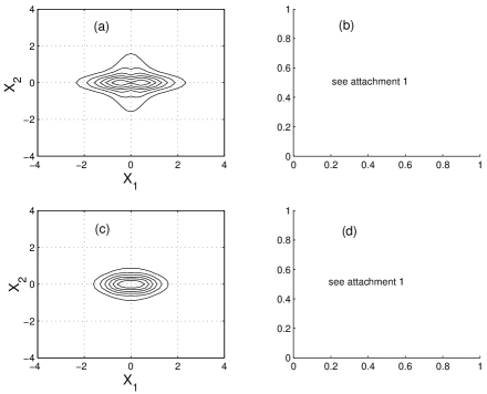
FIG. 6.: Wigner functions of the steady states produced with simple feedback for $\chi=\pi/2$. Figs. (a) and (b) have $\lambda=2.2$, while (c) and (d) have $\lambda=0.97$. The mesh plots are included to aid the readers interpretation of the contour plots.

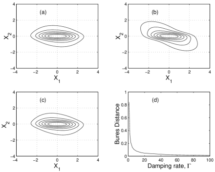
FIG. 7.: Figs. (a), (b) and (c) are Wigner functions of the steady states produced with electro-optic feedback onto a TLA for $\chi=\pi/2$ and $\lambda=2.2$. Fig. (a) is the adiabatically eliminated state. Figs. (b) and (c) represent the full dynamics with $\Gamma=2$ and $20$ respectively. Fig. (d) shows the Bures distance between the adiabatically eliminated state and the state produced with the full dynamics as $\Gamma$ increases.

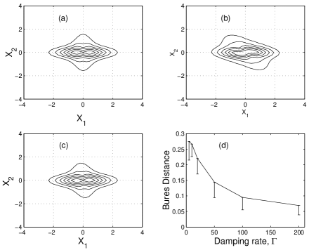
FIG. 8.: Figs. (a), (b) and (c) are Wigner functions of the steady states produced with electro-optic feedback onto a mode for $\chi=\pi/2$ and $\lambda=2.2$. Fig. (a) is the adiabatically eliminated state. Figs. (b) and (c) represent the full dynamics with $\Gamma=10$ and $100$ respectively. Fig. (d) shows the Bures distance between the adiabatically eliminated state and the state produced with the full dynamics as $\Gamma$ increases. The error bars are due to statistical error due to averaging over a less than infinite number of quantum trajectories. Only half error bars are given because, in a high-dimensional Hilbert space, a state with statistical errors will tend to be further away from the adiabatically eliminated state than the true ensemble average will be.

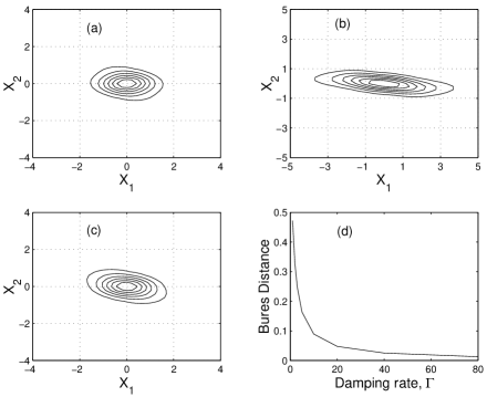
FIG. 9.: Figs. (a), (b) and (c) are Wigner functions of the steady states produced with all-optical feedback onto a TLA for $\chi=\pi/2$ and $\lambda=0.97$. Fig. (a) is the adiabatically eliminated state. Figs. (b) and (c) represent the full dynamics with $\Gamma=1$ and $10$ respectively. Fig. (d) shows the Bures distance between the adiabatically eliminated state and the state produced with the full dynamics as $\Gamma$ increases.

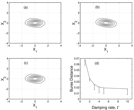
FIG. 10.: Figs. (a), (b) and (c) are Wigner functions of the steady states produced with all-optical feedback onto a mode for $\chi=\pi/2$ and $\lambda=0.97$. Fig. (a) is the adiabatically eliminated state. Figs. (b) and (c) represent the full dynamics with $\Gamma=1$ and $10$ respectively. Fig. (d) shows the Bures distance between the adiabatically eliminated state and the state produced with the full dynamics as $\Gamma$ increases. Half error bars are used for the same reason as in figure 8.

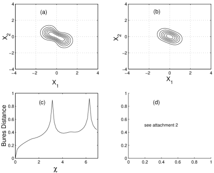
FIG. 11.: The first two plots are Wigner functions of the steady states produced with a $\chi^{(3)}=\pi/2$ non-linearity. Figs. (a) and (b) have driving strengths of $\lambda=2.2$ and $0.97$ respectively. Fig. (c) shows the Bures distance between simple and “reversible” feedback for $\lambda=0.97$. Fig. (d) is a mesh plot of the Wigner function displayed in Fig. (a).

FIG. 12.: Schematic representation of all-optical feedback onto a very large number of optical cavities that are coupled back to the system. The $j^{{\rm th}}$ ancilla cavity has damping rate $\Gamma$ and annihilation operator $b_{j}$.

REFERENCES

- [1] H.M. Wiseman and G.J. Milburn, Phys. Rev. Lett. 70, 548 (1993).
- [2] H.M. Wiseman and G.J. Milburn, Phys. Rev. A 49, 1350 (1994).
- [3] H.M. Wiseman, Phys. Rev. A 49, 2133 (1994); Errata ibid., 49 5159 (1994) and ibid. 50, 4428 (1994).
- [4] H.M. Wiseman and G.J. Milburn, Phys. Rev. A 49, 4110 (1994).
- [5] G. Lindblad, Commun. Math. Phys. 48, 199 (1976).
- [6] S. Lloyd, quant-ph/9703042, to be published in Phys. Rev. A (2000).
- [7] J.J. Slosser and G.J. Milburn, Phys. Rev. A 50, 793 (1994).
- [8] For example, the in-loop spectrum in Ref. [7] is not correct because it does not take into account the correction due to feedback as in Eq. (2.62) of Ref. [3]. Another paper [9] by the same authors also considering feedback in a compound system with adiabatic elimination has worse problems: the central equation (9) is not even dimensionally correct.
- [9] J.J. Slosser and G.J. Milburn, Phys. Rev. Lett. 75, 418 (1995).
- [10] A.C. Doherty, A.S. Parkins, S.M. Tan, and D.F. Walls, Phys. Rev. A 57, 4804 (1998).
- [11] H. J. Carmichael, An Open Systems Approach to Quantum Optics (Springer, Berlin 1993).
- [12] C. W. Gardiner and M. J. Collett, Phys. Rev. A 31, 3761 (1985).
- [13] R. L. Liboff, Introductory Quantum Mechanics (Addison Wesley, Sydney, 1998).
- [14] C. W. Gardiner, Quantum Noise (Springer-Verlag, Berlin, 1991).
- [15] C. W. Gardiner, Handbook of Stochastic Methods (Springer-Verlag, Berlin, 1985).
- [16] H. J. Carmichael, Phys. Rev. Lett. 70 2273 (1993).
- [17] C. W. Gardiner, Phys. Rev. Lett. 70, 2269 (1993).
- [18] D. Bures, Trans. Am. Math. Soc. 135, 199 (1969).
- [19] D. F. Walls and G. J. Milburn, Quantum Optics (Springer, Berlin 1994).
- [20] An accurate simulation is taken to mean .
- [21] Quantum Optics Toolbox, Version 0.10 11-Jan-1999 (University of Auckland); see S.M. Tan, J. Opt. B 1, 424 (1999).
- [22] S. L. Braunstein and C. M. Caves, Phys. Rev. Lett. 72, 3439 (1994).
- [23] P. A. M. Dirac, Proc. R. Soc. Lond. A 114, 243 (1927).
- [24] C. W. Gardiner, A. S. Parkins, and P. Zoller, Phys. Rev. A 46, 4363 (1992).
- [25] J. Dalibard, Y. Castin and K. Mølmer Phys. Rev. Lett. 68, 580 (1992).
- [26] P. D. Drummond and D. F. Walls, J. Phys. A 13, 725 (1980).