Bayesian Reconstruction of Approximately Periodic Potentials at Finite Temperature

Abstract

The paper discusses the reconstruction of potentials for quantum systems at finite temperatures from observational data. A nonparametric approach is developed, based on the framework of Bayesian statistics, to solve such inverse problems. Besides the specific model of quantum statistics giving the probability of observational data, a Bayesian approach is essentially based on a priori information available for the potential. Different possibilities to implement a priori information are discussed in detail, including hyperparameters, hyperfields, and non–Gaussian auxiliary fields. Special emphasis is put on the reconstruction of potentials with approximate periodicity. The feasibility of the approach is demonstrated for a numerical model.

1 Introduction

A successful application of quantum mechanics to real world systems relies essentially on an adequate reconstruction of the underlying potential, describing the forces governing the system. The reconstruction of potentials or forces from available observational data defines an empirical learning task. It also constitutes a typical example of an inverse problem. Such problems are notoriously ill–defined in the sense of Tikhonov Tikhonov-Arsenin-1977 ; Kirsch-1996 ; Vapnik-1998 ; Honerkamp-1998 . In that case additional a priori information is required to yield a unique and stable solution. A Bayesian framework is especially well suited to include both, observational data and a priori information, in a quite flexible manner.

Inverse scattering theory Newton-1989 ; Chadan-Sabatier-1989 ; Chadan-Colton-Paivarinta-Rundell-1997 and inverse spectral theory Gelfand-Levitan-1951 ; Kac-1966 ; Marchenko-1986 ; Zakhariev-Chabanov-1997 are two classical research fields which deal in particular with the reconstruction of potentials from spectral data. Both theories describe the kind of data which are necessary, in addition to a given spectrum, to determine a potential uniquely. In inverse scattering theory these additional data are for example phase shifts, obtained far away from the scatterer. For the bound state problems studied in inverse spectral theory these additional data may consist of a second spectrum obtained for boundary conditions different from those for the first spectrum. The approach of Bayesian Inverse Quantum Mechanics (BIQM) we will refer to in the following is not exclusively designed for spectral data but is able to work with quite arbitrary observational data Lemm-IQS-2000 . It can thus be easily adapted to a large variety of different reconstruction scenarios Lemm-BFT-1999 ; Lemm-TDQ-2000 ; Lemm-IHF-2000 .

The basics of a Bayesian framework are summarized in Section 2. Setting up a Bayesian approach for a specific application area requires the definition of two basic probabilistic models. First, a likelihood model is needed giving, for each possible potential, the probability of the observational data. The likelihood model of quantum statistics is discussed in Section 3. Second, a prior model has to be chosen to implement available a priori information. Prior models which are useful for inverse quantum statistics are presented in Section 4. Technically the most convenient prior models are Gaussian processes, presented in Section 4.1. Section 4.2 shows how covariance and mean of a Gaussian process can be related to a priori information about approximate symmetries of the potentials to be reconstructed. Section 4.3 concentrates on approximate periodicity, Section 4.4 on potentials with discontinuities. Prior models are made more flexible by using hyperparameters (Section 4.5), or more general hyperfields, being function hyperparameters (Section 4.6). Related non–Gaussian priors are the topic of Section 4.7. Having defined liklihood and prior models Section 5 discusses the equations to be solved for reconstructing a potential. Finally, Section 6 presents numerical applications.

2 Bayesian approach

Empirical learning is based on observational data $D$. In particular, we will distinguish “dependent” variables $x$, representing measurement results, and “independent” variables $O$, characterizing the kind of measurement performed. In the context of inverse quantum mechanics the latter denotes the observables which are measured. Such observables may for example be the position, the momentum, or the energy of a quantum particle. Variables $x$ and $O$ are assumed to be measurable and represent therefore visible variables. Observational data will be assumed to consist of $n$ pairs $D$ = $\{(x_{i},O_{i})|1\leq i\leq n\}$ = $(x_{T},O_{T})$, where $x_{T}$ and $O_{T}$ denote the vectors with components $x_{i}$ or $O_{i}$, respectively. Such data will also be called training data. In empirical learning one tries to extract a “general law” from observations. In this paper the quantum potential $V$ to be reconstructed will represent this “general law”. (Similarly, in the Bayesian reconstruction of quantum states the object to be reconstructed is the density operator of an unknown state Helstrom:1976 ; Holevo:1982 ; Tan:1997 ; Buzek-Drobny-Derka-Adam-Wiedemann:1998 .) Potentials, considered not to be directly observable, represent in our context the hidden or latent variables. We will now use the Bayesian framework to relate unobservable potentials to observational data.

The Bayesian approach is a general probabilistic framework to deal with empirical learning problems Bayes-1763 ; Berger-1980 ; Loredo-1990 ; Bernado-Smith-1994 ; Gelman-Carlin-Stern-Rubin-1995 ; Sivia-1996 ; Carlin-Louis-1996 ; Lemm-BFT-1999 . Predicting results of future measurements on the basis of given training data is achieved by means of the predictive probability $p(x|O,D)$ (or predictive density for continuous $x$), which is the probability of finding the value $x$ when measuring observable $O$ under the condition that the training data $D$ are given. To calculate the predictive probability a probabilistic model is needed which describes the measurement process. Such a model is specified by giving the probability $p(x|O,V)$ of finding $x$ when measuring observable $O$ for each possible potential $V$. As $p(x|O,V)$, considered as function of $V$ for fixed $x$ and $O$, is known as likelihood of $V$, we will call this the likelihood model. For inverse quantum problems the likelihood model is given by the axioms of quantum mechanics and will be discussed in Section 3.

According to the rules of probability theory the predictive probability can now be written as an integral over the space of all possible potentials $V$,

$$p(x|O,D)=\int\!dV\,p(x|O,V)\,p(V|D).$$ (1)

We note that in Eq.(1) we have assumed that the probability of $x$ is completely determined by giving potential and observable and does not depend on the training data, $p(x|O,V,D)$ = $p(x|O,V)$, and that the probability of the potential given the training data does not depend on the observables selected in the future, $p(V|O,D)$ = $p(V|D)$. If the set of possible potentials is a space of functions, the integral in (1) is a functional integral.

As the likelihood model is assumed to be given, learning consists in the determination of $p(V|D)$, known as the posterior for $V$. To this end, we relate the posterior for $V$ to the likelihood of $V$ under the training data by applying Bayes’ theorem,

$$p(V|D)=\frac{p(x_{T}|O_{T},V)\,p(V)}{p(x_{T}|O_{T})},$$ (2)

assuming $p(V|O_{T})$ = $p(V)$, analogous to Eq. (1). In the numerator of Eq. (2) appears, besides the likelihood, the so called prior $p(V)$. This prior gives the probability of $V$ before training data have been collected. Hence it has to comprise all a priori information available for the potential. The need for a prior model, complementing the likelihood model, is characteristic for a Bayesian approach. The denominator in Eq. (2) plays the role of a normalization factor and can be obtained from likelihood and prior by integration over $V$ as $p(x_{T}|O_{T})$ = $\int\!dV\,p(x_{T}|O_{T},V)\,p(V)$.

From a Bayesian perspective learning appears as updating the probability for $V$ caused by the arrival of new data $D$. If more data become available this process can be iterated, the old posterior becoming the new prior which is then updated yielding a new posterior.

In practice, a major difficulty is the calculation of the integral over all possible $V$ to get the predictive probability (1). Even if one resorts to a discrete approximation for $x$ the integral (1) is typically still very high dimensional. The key point is thus to find a feasible approximation for that integral. Two approaches are common in Bayesian statistics. The first one is an evaluation of the integral by Monte Carlo methods Gelman-Carlin-Stern-Rubin-1995 ; Metropolis-Rosenbluth-Rosenbluth-Teller-Teller-1953 ; Binder-Heermann-1988 ; Neal-1997 . The second one, which we will pursue in the following, is the so called maximum a posteriori approximation (MAP), being a variant of the saddle point method Berger-1980 ; Gelman-Carlin-Stern-Rubin-1995 ; De-Bruijn-1981 ; Bleistein-Handelsman-1986 ; Girosi-Jones-Poggio-1995 ; Lemm-1996 ; Lemm-1998 . In MAP one assumes the posterior to be sufficiently peaked around the potential $V^{*}$ which maximizes the posterior, so that approximately

$$p(x|O,D)\approx p(x|O,V^{*}),$$ (3)

with

$$V^{*}={\rm argmax}_{V\in{\cal V}}p(V|D)={\rm argmax}_{V\in{\cal V}}p(x_{T}|O_{T},V)p(V).$$ (4)

Maximizing the posterior with respect to $V\in{\cal V}$ means, according to Eq. (2) with the denominator independent of $V$, maximizing the product of likelihood and prior.

The Bayesian framework discussed so far can analogously be applied to a variety of different contexts, including regression, density estimation and classification problems Lemm-BFT-1999 . The case of a Gaussian likelihood with fixed variance, for example, is known as regression problem, while problems with general likelihoods are known as density estimation.

3 Likelihood model of quantum statistics

The first step in applying the Bayesian framework to inverse problems of quantum mechanics or quantum statistics is the definition of the likelihood model Lemm-IQS-2000 . This is easily obtained from the axioms of quantum mechanics. Consider a system prepared in a state described by a density operator $\rho$. As our aim will be to reconstruct potentials $V$ from observational data, we have to choose a $\rho$ which depends on the potential. The probability to find value $x$, when measuring an observable represented by the Hermitian operator $O$, is given by

$$p(x|O,V)={\rm Tr}\Big{(}P_{O}(x)\,\rho(V)\Big{)},$$ (5)

where $P_{O}(x)$ = $\sum_{\zeta}\mbox{$|\,x,\zeta\rangle\langle x,\zeta\,|$}$ denotes the projector on the space of (orthonormalized) eigenfunctions $|x,\zeta\rangle$ of $O$ with eigenvalue $x$ and the variable $\zeta$ distinguishes eigenfunctions with degenerate eigenvalues.

In particular, for a canonical ensemble at temperature $1/\beta$ (setting Boltzmann’s constant equal to 1) the density operator reads

$$\rho=\frac{e^{-\beta H}}{{\rm Tr\,}e^{-\beta H}}.$$ (6)

To be specific, we will study in the following Hamiltonians of the form $H$ = $T+V$, with kinetic energy $T$ = $-(1/2m)\Delta$, (with Laplacian $\Delta$, mass $m$, and setting $\hbar$ = $1$) and a local potential

$$V(x,x^{\prime})=v(x)\delta(x-x^{\prime}),$$ (7)

defined by the function $v(x)$. Note that the formalism presented in the following works with nonlocal potentials as well, numerical calculations, however, would in that case be more demanding. For the likelihood models corresponding to time–dependent quantum systems and to many–body systems in Hartree–Fock approximation we refer to Lemm-TDQ-2000 ; Lemm-IHF-2000 .

In the following we will study observational data consisting of $n$ position measurements $x_{i}$. This corresponds to choosing the position operator for the observables $O_{i}$ = $\hat{x}$ with $\hat{x}\mbox{$|x_{i}\rangle$}$ = $x_{i}\mbox{$|x_{i}\rangle$}$. Hence, for a canonical ensemble, the likelihood (5) becomes for a single position measurement

$$p(x_{i}|\hat{x},v)=\sum_{\alpha}p_{\alpha}|{\phi}_{\alpha}(x_{i})|^{2}=\mbox{$\langle\,|{\phi}(x_{i})|^{2}\,\rangle$}$$ (8)

with (non–degenerate) eigenfunctions ${\phi}_{\alpha}$ of $H$ and energies $E_{\alpha}$, i.e., $H\mbox{$|{\phi}_{\alpha}\rangle$}$ = $E_{\alpha}\mbox{$|{\phi}_{\alpha}\rangle$}$. Angular brackets $\langle\,\cdots\,\rangle$ denote a thermal expectation under the probabilities $p_{\alpha}$ = $\exp(-\beta E_{\alpha})/Z$ with $Z$ = $\sum_{\alpha}\exp(-\beta E_{\alpha})$ according to Eq. (6). For independent data $D_{i}$ = $(x_{i},O_{i})$,

$$p(x_{T}|O_{T},v)=\prod_{i=1}^{n}p(x_{i}|\hat{x},v)=\prod_{i=1}^{n}\mbox{$\langle\,|{\phi}(x_{i})|^{2}\,\rangle$}.$$ (9)

A quantum mechanical measurement changes the state of the system, i.e., it changes $\rho$. Hence, to obtain independent data under constant $\rho$ requires the density operator to be restored before each measurement. For a canonical ensemble this means to wait between two consecutive observations until the system is thermalized again.

Choosing a parametric family of potentials $v(x;\xi)$ one could now maximize the likelihood with respect to the parameters $\xi$, and choose as reconstructed potential

$$v^{*}(x)=v(x;\xi^{*})\quad\mbox{with}\quad\xi^{*}=\mbox{\rm argmax}_{\xi}\,p(x_{T}|O_{T},v(\xi)).$$ (10)

This is known as maximum likelihood approximation and works well if the number of data is large compared to the flexibility of the selected parametric family of potentials. This method does however not yield a unique optimal potential if the flexibility is too large for the available number of observations. (A possible measure of the “flexibility” of a parametric family is given by the Vapnik-Chervonenkis dimension Vapnik-1998 or variants thereof.) In such cases, the inclusion of additional restrictions on $v$ in form of a priori information is essential. This holds especially for nonparametric approaches, where each number $v(x)$ is treated as individual degree of freedom. Including a priori information generalizes the maximum likelihood approximation of Eq. (10) to the MAP of Eq. (4).

4 Prior models

4.1 Gaussian processes

A finite number of observational data cannot completely determine a function $v(x)$. Hence, besides observational data, additional a priori information is necessary to reconstruct a potential in BIQM. In nonparametric approaches it is advantageous to formulate a priori information directly in terms of the function $v(x)$ itself. A convenient choice for a prior is a Gaussian process,

$$p(v)=\left(\det\frac{{\bf K}_{0}}{2\pi}\right)^{\frac{1}{2}}e^{-\frac{1}{2}\langle v-v_{0}\,|\,{\bf K}_{0}\,|\,v-v_{0}\rangle},$$ (11)

where

$$\langle v-v_{0}\,|\,{\bf K}_{0}\,|\,v-v_{0}\rangle=$$ (12)

$$\int\!dx\,dx^{\prime}\,[v(x)-v_{0}(x)]{\bf K}_{0}(x,x^{\prime})[v(x^{\prime})-v_{0}(x^{\prime})].$$

The function $v_{0}$ is the mean or regression function, representing a reference potential or template for $v$. The inverse covariance ${\bf K}_{0}$ is a real symmetric, positive (semi)definite operator which acts on potentials rather than on wave functions and defines a distance measure on the space of potentials. For technical convenience one may introduce explicitly a factor $\lambda$ multiplying ${\bf K}_{0}$ to balance the influence of the prior against the likelihood term. A Gaussian prior as in Eq. (11) is already a quite flexible tool for implementing a priori knowledge. A bias towards smooth functions $v(x)$, for instance, can be implemented by choosing the negative Laplacian as inverse covariance ${\bf K}_{0}$ = $-\Delta$. Including higher derivatives in ${\bf K}_{0}$ would result in even smoother potentials, in the sense that higher derivatives of $v(x)$ become continuous. For example, a common smoothness prior used for regression problems is the Radial Basis Function prior ${\bf K}_{0}$ = $\exp{(-{\sigma_{\rm RBF}^{2}}{\Delta}/2)}$ Girosi-Jones-Poggio-1995 .

4.2 Covariances and approximate symmetries

Prior information on potentials $v$ can often be related to approximate invariance under specific transformations Lemm-BFT-1999 . Typical examples of such transformations are symmetry operations like translations or rotations. To be specific, assume that a (not necessarily local) potential $V$ commutes approximately, but not exactly, with some unitary operator $S$,

$$V\approx S^{\dagger}VS={\bf S}V,$$ (13)

which defines an operator ${\bf S}$ acting on $V$. In particular, we may choose a prior $p(V)\propto\exp\{-E_{S}(V)\}$ with a prior energy

$$E_{S}=\frac{1}{2}\mbox{$\langle V-{\bf S}V\,|\,V-{\bf S}V\rangle$}=\frac{1}{2}\langle V\,|\,{\bf K}_{0}\,|\,V\rangle.$$ (14)

This shows that the expectation of an approximate symmetry of $V$ under $S$ can be implemented by choosing a Gaussian prior with inverse covariance operator

$${\bf K}_{0}=({\bf I}-{\bf S})^{\dagger}({\bf I}-{\bf S}),$$ (15)

where ${\bf I}$ denotes the identity operator. Symmetry operations $S(\theta)$, with corresponding ${\bf S}(\theta)$, may depend on a parameter (vector) $\theta$. Approximate invariance under $S(\theta_{i})$ for several $\theta_{i}$ can be implemented by using the sum (or integral, for continuous variables)

$$E_{S} = \frac{1}{2}\sum_{i}\mbox{$\langle V-{\bf S}(\theta_{i})V\,|\,V-{\bf S}(\theta_{i})V\rangle$}$$ (16)

$$= \frac{1}{2}\sum_{i}\langle V\,|\,{\bf K}_{0}(\theta_{i})\,|\,V\rangle.$$

Alternatively, one may require approximate symmetry for only one value of $\theta$, not fixed a priori. For example, one may expect an approximately periodic potential with unknown periodicity length $\theta$ which also has to be determined from the data. Such $\theta$ are known as hyperparameters and will be discussed in Section 4.5.

Lie groups are continuously parameterized transformations

$${\bf S}(\theta)=e^{\sum_{i}\theta_{i}{\bf s}_{i}},$$ (17)

where $\theta_{i}$ are the real parameters and the ${\bf s}_{i}$ = $-{\bf s}_{i}^{T}$ (the superscript ^T denoting the transpose) are antisymmetric operators representing the generators of the infinitesimal transformations of the Lie–group. We can define a prior energy as an error measure with respect to an infinitesimal transformation,

$$E_{S} = \frac{1}{2}\sum_{i}\Big{\langle}\frac{{V}-(1+\theta_{i}{\bf s}_{i}){V}}{\theta_{i}}\,\Big{|}\,{\frac{{V}-(1+\theta_{i}{\bf s}_{i}){V}}{\theta_{i}}}\Big{\rangle}$$ (18)

$$= \frac{1}{2}\langle{V}\,|\,\sum_{i}{\bf s}_{i}^{T}{\bf s}_{i}\,|\,{V}\rangle.$$

For instance, a Laplacian smoothness prior for a local potential $v(x)$ can be related to an approximate symmetry under infinitesimal translations. For the group of $d$–dimensional translations which is generated by the gradient operator $\nabla$ this can be verified by recalling the multidimensional Taylor formula for expanding ${v}$ around $x$

$${\bf S}(\theta){v}(x)=e^{\sum_{i}\theta_{i}\nabla_{i}}{v}(x)=\sum_{k=0}^{\infty}\frac{\left(\sum_{i}\theta_{i}\nabla_{i}\right)^{k}}{k!}{v}(x)={v}(x+\theta).$$ (19)

Up to first order ${\bf S}\approx 1+\sum_{i}\theta_{i}\nabla_{i}$. Hence, for infinitesimal translations, the error measure of Eq. (18) becomes

$$E_{S} = \frac{1}{2}\sum_{i}\Big{\langle}\frac{{v}-(1+\theta_{i}{\nabla}_{i}){v}}{\theta_{i}}\,\Big{|}\,{\frac{{v}-(1+\theta_{i}{\nabla}_{i}){v}}{\theta_{i}}}\Big{\rangle}$$ (20)

$$= -\frac{1}{2}\langle{v}\,|\,\Delta\,|\,{v}\rangle,$$

assuming vanishing boundary terms. This is the classical Laplacian smoothness term.

4.3 Approximate periodicity

In this paper we will in particular be interested in potentials which are approximately periodic. To measure the deviation from exact periodicity for a local potential $v(x)$ let us define the difference operators

$$\left(\nabla^{R}_{\theta}v\right)(x) = {v}(x+\theta)-{v}(x).$$ (21)

$$\left(\nabla^{L}_{\theta}v\right)(x) = {v}(x)-{v}(x-\theta),$$ (22)

For periodic boundary conditions $(\nabla^{L}_{\theta})^{T}$ = $-\nabla^{R}_{\theta}$, where $(\nabla^{L}_{\theta})^{T}$ denotes the transpose of $\nabla^{L}_{\theta}$. Hence, the operator

$$-\Delta_{\theta}=-\nabla^{L}_{\theta}\nabla^{R}_{\theta}=(\nabla^{R}_{\theta})^{T}\nabla^{R}_{\theta}$$ (23)

defined in analogy to the negative Laplacian, is positive (semi)definite, and a possible prior energy is an error term which measures the deviation from exact periodicity for given period $\theta$,

$$E_{S} = \frac{1}{2}\int\!dx\;|{v}(x)-{v}(x+\theta)|^{2}$$ (24)

$$= \frac{1}{2}\mbox{$\langle\nabla^{R}_{\theta}{v}\,|\,\nabla^{R}_{\theta}{v}\rangle$}$$

$$= -\frac{1}{2}\langle{v}\,|\,\Delta_{\theta}\,|\,{v}\rangle.$$

Discretizing $v$ the operator $\nabla^{R}_{\theta}$ for periodic boundary conditions becomes, for example on a mesh with six points and $\theta$ = $2$, the matrix

$$\nabla^{R}_{\theta}=\left(\begin{tabular}[]{ c c c c c c }$-1$&0&$1$&0&0&0\\ 0&$-1$&0&$1$&0&0\\ 0&0&$-1$&0&$1$&0\\ 0&0&0&$-1$&0&$1$\\ $1$&0&0&0&$-1$&0\\ 0&$1$&0&0&0&$-1$\\ \end{tabular}\right),$$ (25)

so that

$$-\Delta_{\theta}=\left(\begin{tabular}[]{ c c c c c c }2&0&$-1$&0&$-1$&0\\ 0&2&0&$-1$&0&$-1$\\ $-1$&0&2&0&$-1$&0\\ 0&$-1$&0&2&0&$-1$\\ $-1$&0&$-1$&0&2&0\\ 0&$-1$&0&$-1$&0&2\\ \end{tabular}\right).$$ (26)

As every periodic function with ${v}(x)={v}(x+\theta)$ is in the null space of $\Delta_{\theta}$ typically another error term has to be added to get a unique maximum of the posterior. For example, combining a prior energy (24) with a Laplacian smoothness term yields a Gaussian prior of the form (11) with inverse covariance ${\bf K}_{0}$ = $-\lambda(\Delta+\gamma\Delta_{\theta})$ and prior energy

$$E_{S}=-\frac{\lambda}{2}\langle{v}\,|\,\Delta+\gamma\Delta_{\theta}\,|\,{v}\rangle,$$ (27)

with weighting factors $\lambda$, $\gamma$. In case the period $\theta$ is not known, it can be treated as hyperparameter as will be discussed in Section 4.5. Clearly, a nonzero reference potential $v_{0}$ can be included in Eq. (27). In Eq. (24), one may also sum over several periods

$$E_{S}=\frac{1}{2}\sum_{k=1}^{k_{\rm max}}w(k)\int\!dx\;|{v}(x)-{v}(x+k\theta)|^{2},$$ (28)

where $w(k)$ is a weighting function, decreasing for larger $k$. Prior energies as in (28) enforce approximate periodicity over longer distances than a prior energy of the form (24). The latter, on the other hand, is more robust than (28) with respect to local deviations from periodicity, like a locally varying frequency.

Instead of choosing an inverse covariance ${\bf K}_{0}$ with symmetric functions in its null space, approximate symmetries can be implemented by using explicitly a symmetric reference function $v_{0}$ = ${\bf S}v_{0}$ for the Gaussian prior (11). For approximate periodicity, this would mean to choose a periodic reference potential $v_{0}(x)$ = $v_{0}(x+\theta)$ in the prior energy $E_{S}=\frac{1}{2}\langle{v}-v_{0}\,|\,{\bf K}_{0}\,|\,{v}-v_{0}\rangle$ where ${\bf K}_{0}$ could be for example the identity or a differential operator. Thus a periodic reference potential favors a specific form for the reconstructed potential, including a specific frequency and phase. This is different for the covariance implementation (24) of approximate periodicity where only the frequency is relevant and reference potentials can still be chosen arbitrarily. They may, for example be nonperiodic functions or functions with even higher symmetry like in Eq. (27) where $v_{0}\equiv 0$ is invariant under all translations. Flexible reference potentials will be studied in Section 4.5.

4.4 Potentials with discontinuities

Smooth potentials $v(x)$ with discontinuities can either be approximated by using discontinuous templates $v_{0}(x;\theta)$ or by eliminating matrix elements of the inverse covariance which connect the two sides of the discontinuity. For example, consider the discrete version of a negative Laplacian with unit lattice spacing and periodic boundary conditions,

$${\bf K}_{0}=-\Delta=\left(\begin{tabular}[]{ c c c c c c }2&$-1$&0&0&0&$-1$\\ $-1$&2&$-1$&0&0&0\\ 0&$-1$&2&$-1$&0&0\\ 0&0&$-1$&2&$-1$&0\\ 0&0&0&$-1$&2&$-1$\\ $-1$&0&0&0&$-1$&2\\ \end{tabular}\right).$$ (29)

Decomposing the matrix (29) into square roots we write ${\bf K}_{0}$ = ${\bf W}^{T}{\bf W}$ (see also Section 4.6) where a possible square root is

$${\bf W}=\nabla_{1}^{R}=\left(\begin{tabular}[]{ c c c c c c }$-1$&$1$&0&0&0&0\\ 0&$-1$&$1$&0&0&0\\ 0&0&$-1$&$1$&0&0\\ 0&0&0&$-1$&$1$&0\\ 0&0&0&0&$-1$&$1$\\ $1$&0&0&0&0&$-1$\\ \end{tabular}\right).$$ (30)

Similarly, the derivative operator $\partial/\partial x$ represents a square root of the negative Laplacian for periodic boundary conditions. Two regions can now be disconnected by deleting all lines of ${\bf W}$ which have matrix elements in both regions. For instance, the first three points in the six–dimensional space of Eq. (30) can be disconnected from the last three points by setting ${\bf W}(3,\cdot)$ and ${\bf W}(6,\cdot)$ to zero,

0−11000000000000−1100000−11000000).~𝐖fragments 0fragments11000000000000fragments1100000fragments11000000\tilde{\bf W}=\left(\begin{tabular}[]{ c c c | c c c }$-1$&$1$&0&0&0&0\\ 0&$-1$&$1$&0&0&0\\ 0&0&0&0&0&0\\ \hline\cr 0&0&0&$-1$&$1$&0\\ 0&0&0&0&$-1$&$1$\\ 0&0&0&0&0&0\\ \end{tabular}\right).

−110000−110000 (31)

Squaring of $\tilde{\bf W}$ yields a positive semidefinite operator

−12−10000−110000001−10000−12−10000−11)subscript~𝐊0superscript~𝐖𝑇~𝐖fragments fragments12fragments10000fragments11000fragments0001fragments10000fragments12fragments10000fragments11\tilde{\bf K}_{0}={\tilde{\bf W}}^{T}\tilde{\bf W}=\left(\begin{tabular}[]{ c c c | c c c }1&$-1$&0&0&0&0\\ $-1$&2&$-1$&0&0&0\\ 0&$-1$&1&0&0&0\\ \hline\cr 0&0&0&1&$-1$&0\\ 0&0&0&$-1$&2&$-1$\\ 0&0&0&0&$-1$&1\\ \end{tabular}\right)

1−100001−10000 (32)

resulting in a smoothness prior which is ineffective between points from different regions. In contrast to using discontinuous templates, the height of the jump at the discontinuity has not to be given in advance when working with disconnected Laplacians (or other disconnected inverse covariances). On the other hand training data are then required for all separated regions to determine the free constants which correspond to the zero modes of the local Laplacians. The reconstruction of discontinuous functions with non–Gaussian priors will be discussed in Section 4.7.

4.5 Hyperparameters

Parameters of the prior are known as hyperparameters Lemm-BFT-1999 ; Carlin-Louis-1996 ; Bishop-1995b . Like potentials $v$, hyperparameters $\theta$ are not directly observable and represent hidden variables. In the presence of hyperparameters a prior for $v$ can be decomposed as follows

$$p(v)=\int\!d\theta\,p(v|\theta)\,p(\theta),$$ (33)

where $p(\theta)$ is known as hyperprior. The likelihood does not depend on $\theta$, the predictive probability (1), however, contains then an integral over $\theta$,

$$p(x|O,D)=$$ (34)

$$\frac{1}{p(x_{T}|O_{T})}\int\!dv\,d\theta\,p(x|O,v)\,p(x_{T}|O_{T},v)\,p(v|\theta)\,p(\theta).$$

Like the integral over $v$, the integral over $\theta$ can be calculated either by Monte Carlo methods or in MAP. We remark that, when a $\theta$–dependent prior is written in terms of a corresponding prior energy $p(v|\theta)\propto e^{-E(v|\theta)}$, the normalization $\int\!dv\,e^{-E(v|\theta)}$ is independent of $v$ but does in general depend on $\theta$.

Hyperparameters $\theta$ can be single numbers or vectors. They can describe continuous transformations, like translation, rotation or scaling of template functions and scaling of inverse covariance operators. For real $\theta$ and differentiable posterior, stationarity conditions can be found by differentiating the posterior with respect to $\theta$.

Instead of continuous transformations of templates or inverse covariances one can consider a finite collection of alternative reference potentials $v_{i}$ or alternative inverse covariances ${\bf K}_{i}$. For example, a potential to be reconstructed may be expected to be similar to one reference potential out of a small number of possible alternatives $v_{i}$. The “class” variables $i$ are then nothing else but hyperparameters $\theta$ with integer values.

Binary parameters allow to select from two reference functions or two inverse covariances that one which fits the data best. Indeed, writing

$$v_{0}(\theta) = (1-\theta)v_{1}+\theta v_{2},$$ (35)

$${\bf K}_{0}(\theta) = (1-\theta){\bf K}_{1}+\theta{\bf K}_{2},$$ (36)

a binary $\theta\in\{0,1\}$ implements hard switching between alternative templates or inverse covariances, corresponding to a conditional prior

$$p(v|\theta)\propto e^{-(1-\theta)E_{1}(v)-\theta E_{2}(v)}$$ (37)

with

$$E_{1}(v) = \frac{1}{2}\langle v-v_{1}\,|\,{\bf K}_{1}\,|\,v-v_{1}\rangle,$$ (38)

$$E_{2}(v) = \frac{1}{2}\langle v-v_{2}\,|\,{\bf K}_{2}\,|\,v-v_{2}\rangle.$$ (39)

Similarly, a real $\theta\in[0,1]$ in (35) or (36) yields soft mixing. In that case, however, the mixing of templates in (35) is not equivalent to a mixing of prior energies as in (37) because for real $\theta$ Eqs. (35) and (36) lead to mixed terms, like $(1-\theta)\theta\langle v-v_{1}\,|\,{\bf K}_{0}\,|\,v-v_{2}\rangle/2$ for ${\bf K}_{1}$ = ${\bf K}_{2}$. When $\theta$ takes integer values the integral $\int\!d\theta$ becomes a sum $\sum_{\theta}$ so that prior, posterior, and predictive probability have the form of a finite mixture with components $\theta$ lemm-mixture-1999 .

For a moderate number of components one may be able to include all of the mixture components in the calculations. If the number of mixture components is too large one must select some of the components, for example by creating a random sample using Monte Carlo methods, or by solving for the $\theta^{*}$ with maximal posterior. In contrast to typical optimization problems for real variables, the corresponding integer optimization problems are usually not very smooth with respect to $\theta$ (with smoothness defined in terms of differences instead of derivatives), and are therefore often much harder to solve.

There exists a variety of deterministic and stochastic integer optimization algorithms, which may be combined with ensemble methods like genetic algorithms Holland-1975 ; Goldberg-1989 ; Michalewicz-1992 ; Schwefel-1995 ; Mitchell-1996 , and with homotopy methods like simulated annealing Kirkpatrick-Gelatt-Vecchi-1983 ; Mezard-Parisi-Virasoro-1987 ; Aarts-Korts-1989 ; Gelfand-Mitter-1991 ; Yuille-Kosowski-1994 . Annealing methods are similar to (Markov chain) Monte Carlo methods, which aim at sampling many points from a specific distribution (i.e., for example at fixed temperature). For Monte Carlo methods it is important to have (nearly) independent samples and the correct limiting distribution for the Markov chain. For annealing methods the aim is to find the correct minimum by smoothly changing the temperature from a finite value to zero. For the latter it is thus less important to model the distribution for nonzero temperatures exactly, but it is important to use an adequate cooling scheme for lowering the temperature.

4.6 Hyperfields

The hyperparameters $\theta$ considered so far have been real or integer numbers, or vectors with real or integer components $\theta_{i}$. In this section we will discuss priors parameterized by functions, called hyperfields Lemm-BFT-1999 , resulting in a still larger flexibility of the formalism. In numerical calculations where functions have to be discretized hyperfields stand for high dimensional hyperparameter vectors.

Using hyperfields one has to keep in mind that a gain in flexibility at the same time tends to lower the influence of the prior. For example, consider as hyperfield a completely adaptive reference potential $\theta(x)$ = $v_{0}(x)$ within a Gaussian prior (11). Then, for any $v(x)$ the prior energy vanishes for $v_{0}(x)$ = $v(x)$. In the absence of additional hyperpriors $p(\theta)$ the corresponding MAP solution for the hyperfield $\theta(x)$ = $v_{0}(x)$ is thus $\theta^{*}(x)$ = $v(x)$ for which the Gaussian prior (11) becomes uniform in $v(x)$. Hence the price to be paid for the additional flexibility introduced by hyperfields are weaker priors and a large number of additional degrees of freedom. This can considerably complicate calculations and requires sufficiently restrictive hyperpriors for the hyperfields.

Let us define local hyperfields $\theta(x)$ to be hyperfields depending on the position variable $x$. (In general hyperfields can be introduced which depend on other real variables or on several position variables.) Local hyperfields can be used, for example, to adapt templates or inverse covariances locally. To this end, we express real symmetric, positive (semi)definite inverse covariances by square roots or (real) filter operators ${\bf W}$, so that

$${\bf K}_{0}={\bf W}^{T}{\bf W}.$$ (40)

In components

$${\bf K}_{0}(x,x^{\prime})=\int\!dx^{\prime\prime}\;{\bf W}^{T}(x,x^{\prime\prime}){\bf W}(x^{\prime\prime},x^{\prime}),$$ (41)

and therefore

$$\langle{v}-v_{0}\,|\,{\bf K}_{0}\,|\,{v}-v_{0}\rangle = \int\!dx\,dx^{\prime}\,dx^{\prime\prime}\,[{v}(x)-v_{0}(x)]$$ (42)

$$\times\;{\bf W}^{T}(x,x^{\prime}){\bf W}(x^{\prime},x^{\prime\prime})$$

$$\times\;[{v}(x^{\prime\prime})-v_{0}(x^{\prime\prime})]$$

$$= \int\!dx\,|\omega(x)|^{2},$$

where we define the filtered difference

$$\omega(x)=\int\!dx^{\prime}\,{\bf W}(x,x^{\prime})[{v}(x^{\prime})-v_{0}(x^{\prime})].$$ (43)

For instance, a square root (30) of the discrete negative Laplacian (29) corresponds for $v_{0}\equiv 0$ to a filtered difference $\omega(x)$ = $v(x+1)-v(x)$.

The exponent of a Gaussian prior for a local potential ${v}$ can thus be written as an integral over $x$,

$$p({v})\propto e^{-E(v)};\quad E(v)=\frac{1}{2}\int\!dx\,|\omega(x)|^{2}.$$ (44)

In contrast to Eqs. (35) and (36) the representation (44) is well suited for introducing local hyperfields. For instance, an adaptive prior

$$p({v}|\theta)=e^{-E(v|\theta)},$$ (45)

with a real local hyperfield $\theta(x)\in[0,1]$ can be obtained by mixing locally two alternative filtered differences

$$\omega(x;\theta)=[1-\theta(x)]\,\omega_{1}(x)+\theta(x)\,\omega_{2}(x),$$ (46)

where the two $\omega_{i}$ may differ in their filters and/or reference potentials. In that case the hyperfield $\theta(x)$ can locally select the best mixture of the filtered differences $\omega_{i}$, i.e., that one which yields in (45) the largest probability or smallest prior energy

$$E(v|\theta) = \frac{1}{2}\int\!dx|\omega(x;\theta)|^{2}+\ln Z_{\cal V}(\theta)$$

$$= \frac{1}{2}\!\int\!\!dx\Big{|}[1-\theta(x)]\omega_{1}(x)+\theta(x)\omega_{2}(x)\Big{|}^{2}\!+\ln Z_{\cal V}(\theta).$$

Here the normalization factor

$$Z_{\cal V}(\theta)=\int_{v\in{\cal V}}d\!v\,e^{-\frac{1}{2}\int\!dx|\omega(x;\theta)|^{2}},$$ (48)

depends in general on $\theta$ if the filters of the $\omega_{i}$ differ. Clearly, allowing an unbounded $-\infty\leq\theta(x)\leq\infty$ any function $\omega(x;\theta)$ can be written in the form of Eq. (46), provided $\omega_{1}(x)\neq\omega_{2}(x)$ for all $x$.

In contrast to soft mixing with real functions $\theta(x)$ a binary local hyperfield $\theta(x)\in\{0,1\}$ implements hard switching between alternative filtered differences. Since in the binary case $\theta^{2}$ = $\theta$, $(1-\theta)^{2}$ = $(1-\theta)$, and $\theta(1-\theta)$ = $0$, Eq. (4.6) becomes [compare Eq. (37)]

$$E({v}|\theta) = \frac{1}{2}\int\!dx\,\Big{(}[1-\theta(x)]|\omega_{1}(x)|^{2}$$ (49)

$$\quad+\theta(x)|\omega_{2}(x)|^{2}\Big{)}+\ln Z_{\cal V}(\theta),$$

while for real $\theta(x)$ Eq. (4.6) includes a mixed term in $\omega_{1}\omega_{2}$. It is sometimes helpful to transform an unrestricted real hyperfield $-\infty\leq g(x)\leq\infty$ into a bounded real hyperfield $\theta(x)\in[0,1]$ by

$$\theta(x)=\sigma(g(x)-\vartheta),$$ (50)

with threshold $\vartheta$ and sigmoidal transformation

$$\sigma(x)=\frac{1}{1+e^{-2\nu x}}=\frac{1}{2}(\tanh(\nu x)+1).$$ (51)

In the limit $\nu\rightarrow\infty$ the transformation $\sigma(x)$ of (51) approaches the step function $\Theta(x)$ and (50) results in a binary $\theta(x)$ = $\Theta(g(x)-\vartheta)\in\{0,1\}$.

Analogous to the global mixing or global switching in Eq. (35) and Eq. (36), the alternative filtered differences $\omega_{i}(x)$ at position $x$ in Eq. (46) can be constructed by local mixing or switching between template functions $v_{1}(x^{\prime})$, $v_{2}(x^{\prime})$ or filters ${\bf W}_{1}(x,x^{\prime})$, ${\bf W}_{2}(x,x^{\prime})$ using a local hyperfield $\theta(x)$,

$$v_{x}(x^{\prime};\theta) = [1-\theta(x)]\,v_{1}(x^{\prime})+\theta(x)\,v_{2}(x^{\prime}),$$ (52)

$${\bf W}(x,x^{\prime};\theta) = [1\!-\theta(x)]{\bf W}_{1}(x,x^{\prime})\!+\theta(x){\bf W}_{2}(x,x^{\prime}).\;\;$$ (53)

It is important to note that the local templates or reference potentials $v_{x}(x^{\prime};\theta)$ are functions of $x^{\prime}$ and $x$. Indeed, to obtain a filtered difference $\omega(x;\theta)$ at position $x$, a reference function $v_{x}$ is needed for all $x^{\prime}$ for which the corresponding ${\bf W}(x,x^{\prime})$ is nonzero, since

$$\omega(x;\theta)=\int\!dx^{\prime}\,{\bf W}(x,x^{\prime})[{v}(x^{\prime})-v_{x}(x^{\prime};\theta)].$$ (54)

In this way the whole template function $v_{x}(x^{\prime};\theta)$, rather than individual function values $v_{0}(x,\theta)$, is adapted individually for every local filtered difference. In particular, the local reference potentials of Eq. (52) have to be distinguished from one global, locally adapted reference potential

$$v_{0}(x^{\prime};\theta)=[1-\theta(x^{\prime})]\,v_{1}(x^{\prime})+\theta(x^{\prime})\,v_{2}(x^{\prime}),$$ (55)

which at first glance seems to be the natural generalization of Eq. (35) to local hyperfields. Only in Gaussian prior terms with the identity ${\bf I}$ as covariance, local template functions $v_{x}(x^{\prime},\theta)$ are not required. In that case $v_{x}(x^{\prime};\theta)$ is only needed for $x$ = $x^{\prime}$ and we may directly write $v_{x}(x^{\prime};\theta)$ = $\tilde{v}_{0}(x^{\prime};\theta)$, skipping the variable $x$, and obtain the prior energy

$$\frac{1}{2}\int\!dx\;|\omega(x;\theta)|^{2}=\frac{1}{2}\mbox{$\langle v-\tilde{v}_{0}(\theta)\,|\,v-\tilde{v}_{0}(\theta)\rangle$}.$$ (56)

We remark that one can also generalize Eq. (52), which uses the same $v_{1}(x^{\prime})$, $v_{2}(x^{\prime})$ for all $x$, by working with reference potentials $v_{1,x}(x^{\prime})$, $v_{2,x}(x^{\prime})$ which vary with the position $x$ at which the filtered difference $\omega(x)$ is required. This yields

$$v_{x}(x^{\prime};\theta)=[1-\theta(x)]\,v_{1,x}(x^{\prime})+\theta(x)\,v_{2,x}(x^{\prime}).$$ (57)

For binary $\theta(x)$ Eq. (53) corresponds to an inverse covariance

$${\bf K}_{0}(\theta) = \int\!dx\;{\bf K}_{x}(\theta)=\int\!dx\,{W}_{x}(\theta){W}^{T}_{x}(\theta)$$ (58)

$$= \int\!\!dx\left([1-\theta(x)]{W}_{1,x}{W}^{T}_{1,x}+\theta(x){W}_{2,x}{W}^{T}_{2,x}\right)\qquad$$

with

$${\bf K}_{x}(\theta)={W}_{x}(\theta){W}^{T}_{x}(\theta)$$ (59)

written as dyadic product of the vector $W_{x}(\theta)$ = ${\bf W}(x,\cdot\,;\theta)$ and with analogously defined $W_{i,x}$ = ${\bf W}_{i}(x,\cdot)$. For $\theta$–dependent inverse covariances the normalization factors $Z_{\cal V}(\theta)$ become $\theta$–dependent. They have to be included when integrating over $\theta$ or solving for the optimal $\theta$ in MAP.

In Eqs. (52) and (53) it is straightforward to introduce two binary hyperfields $\theta$, $\theta^{\prime}$, one for the reference potential $v_{x}$ and one for the filter ${\bf W}$. This results in a conditional prior

$$p({v}|\theta,\theta^{\prime}) \propto e^{-\frac{1}{2}\int\!dx\,\langle{v}-v_{x}(\theta)\,|\,{\bf K}_{x}(\theta^{\prime})\,|\,{v}-v_{x}(\theta)\rangle}$$ (60)

$$= e^{-\frac{1}{2}\int\!dx\,|\omega(x;\theta,\theta^{\prime})|^{2}}.$$

Here we can write

$$\int\!dx\,|\omega(x;\theta,\theta^{\prime})|^{2} = \langle{v}-v_{0}(\theta,\theta^{\prime})\,|\,{\bf K}_{0}(\theta^{\prime})\,|\,{v}-v_{0}(\theta,\theta^{\prime})\rangle$$ (61)

$$+\int\!dx\,\langle v_{x}(\theta)\,|\,{\bf K}_{x}(\theta^{\prime})\,|\,v_{x}(\theta)\rangle$$

$$-\langle v_{0}(\theta,\theta^{\prime})\,|\,{\bf K}_{0}(\theta^{\prime})\,|\,v_{0}(\theta,\theta^{\prime})\rangle,$$

with an effective template $v_{0}(\theta,\theta^{\prime})$ given by

$$v_{0}(\theta,\theta^{\prime})={\bf K}_{0}(\theta^{\prime})^{-1}\int\!dx\,{\bf K}_{x}(\theta^{\prime})\,v_{x}(\theta),$$ (62)

and effective inverse covariance ${\bf K}_{0}(\theta^{\prime})$ = $\int\!dx\,{\bf K}_{x}(\theta^{\prime})$ as in Eq. (58). Since the last two terms in Eq. (61) are ${v}$–independent constants (only depending on $\theta$, $\theta^{\prime}$) we see that for fixed hyperfields this prior is minimized by $v$ = $v_{0}(\theta,\theta^{\prime})$. For given hyperparameters $\theta$, $\theta^{\prime}$ we can write $p({v}|\theta,\theta^{\prime})\propto e^{-E({v}|\theta,\theta^{\prime})}$ with a prior energy of the form $E({v}|\theta,\theta^{\prime})$ = $\frac{1}{2}\langle{v}-v_{0}(\theta,\theta^{\prime})\,|\,{\bf K}_{0}(\theta^{\prime})\,|\,{v}-v_{0}(\theta,\theta^{\prime})\rangle$.

As the product of Gaussians is again a Gaussian several Gaussian prior factors can easily be combined. In this way one can implement a nonlocal property like smoothness and still avoid local template functions $v_{x}(x^{\prime},\theta)$ by combining a Gaussian prior with ${\bf K}_{0}$ = ${\bf I}$ as in (56) with a Gaussian prior with nondiagonal covariance and zero (or fixed) template,

$$E({v}|\theta)=\frac{1}{2}\mbox{$\langle{v}-\tilde{v}_{0}(\theta)\,|\,{v}-\tilde{v}_{0}(\theta)\rangle$}+\frac{1}{2}\langle{v}\,|\,{\bf K}\,|\,{v}\rangle.$$ (63)

Combining both terms yields

$$E({v}|\theta) = \frac{1}{2}\bigg{(}\langle{v}-v_{0}(\theta)\,|\,{\bf K}_{0}\,|\,{v}-v_{0}(\theta)\rangle$$ (64)

$$\quad+\;\;\langle\tilde{v}_{0}(\theta)\,|\,{\bf I}-{\bf K}_{0}^{-1}\,|\,\tilde{v}_{0}(\theta)\rangle\bigg{)},$$

with the second term being independent of $v$ and with effective template and effective inverse covariance

$$v_{0}(\theta)={\bf K}_{0}^{-1}\tilde{v}_{0}(\theta),\quad{\bf K}_{0}={\bf I}+{\bf K}.$$ (65)

For differential operators ${\bf K}_{0}$ the effective $v_{0}(\theta)$ is thus a smoothed version of $\tilde{v}_{0}(\theta)$.

The extreme case would be to treat $v_{0}$ and ${\bf W}$ itself as unrestricted hyperfields. As already discussed, this just eliminates the corresponding prior term. Hence, to restrict the flexibility, typically a smoothness hyperprior may be imposed to prevent highly oscillating functions $\theta(x)$. For real $\theta(x)$, for example, a smoothness prior like a Laplacian prior $\langle\theta\,|\,\!-\!\Delta\,|\,\theta\rangle/2$ can be used in regions where it is defined. (The space of functions for which a smoothness prior with discontinuous templates is defined depends on the locations of the discontinuities.) An example of a non–Gaussian hyperprior is

$$p(\theta)\propto e^{-\frac{\tau}{2}\int\!dx\,C_{\theta}(x)},$$ (66)

where $\tau$ is a constant and

$$C_{\theta}(x)=\sigma\left(\left(\frac{\partial\theta}{\partial x}\right)^{2}-\vartheta_{\theta}\right),$$ (67)

with a sigmoid $\sigma(x)$ as in (51). For $\nu\rightarrow\infty$ the sigmoid approaches a step function and $C_{\theta}(x)$ becomes zero at locations where the square of the first derivative is smaller than a certain threshold $0\leq\vartheta_{\theta}<\infty$, and one otherwise. For discrete $x$ one can analogously count the number of jumps larger than a given threshold. One can then penalize the number $N_{d}(\theta)$ of discontinuities where $\left(\partial\theta/\partial x\right)^{2}$ = $\infty$ and use

$$p(\theta)\propto e^{-\frac{\tau}{2}N_{d}(\theta)}.$$ (68)

In the case of a binary field this corresponds to counting the number of times the field changes its value. The expression $C_{\theta}$ of Eq. (67) can be generalized to

$$C_{\theta}(x)=\sigma\left(|\omega_{\theta}(x)|^{2}-\vartheta_{\theta}\right),$$ (69)

where, analogous to Eq. (43),

$$\omega_{\theta}(x)=\int\!dx^{\prime}\,{\bf W}_{\theta}(x,x^{\prime})[\theta(x^{\prime})-t_{\theta}(x^{\prime})],$$ (70)

with template $t_{\theta}(x^{\prime})$ representing the expected form for the hyperfield, and a filter operator ${\bf W}_{\theta}$ defining a distance measure for hyperfields. Parameters of the hyperprior like $\tau$ in Eq. (66) or Eq. (68) can be treated as higher level hyperparameters.

4.7 Non–Gaussian priors and auxiliary fields

As an alternative to introducing hyperfields $\theta(x)$ one can work with priors which are explicitly non–Gaussian with respect to $v$. This can be done by introducing auxiliary fields $B(x;v)$ whose function values are not considered as independent variables but are directly defined as functionals of $v$. (For the sake of simplicity we will for $B(x;v)$ also write $B(x)$ or $B(v)$, depending on the context.) Like hyperfields, auxiliary fields can select locally the best adapted filtered difference from a set of alternative $\omega_{i}$.

For instance, consider the auxiliary field [compare with Eqs. (50) or (69)]

$$B(x)=\sigma\left(u(x)-\vartheta\right),$$ (71)

where

$$u(x)=|\omega_{1}(x)|^{2}-|\omega_{2}(x)|^{2},$$ (72)

$\vartheta$ represents a threshold, $\sigma(x)$ a sigmoidal function as in (51), and the $\omega_{i}$ are filtered differences defined in terms of $v$ according to Eq. (43). Again a binary field $B(x)$ is obtained by letting the sigmoid approach the step function. Because the $\omega_{i}$ depend on $v$, it is clear from the definition (71) that the auxiliary field $B(x)$ is no independent hyperfield but has values being functionals of ${v}$. Notice that $B(x)$ is nonlocal with respect to ${v}(x)$ if $\omega_{i}(x)$ is nonlocal; a value $B(x)$ then depends on more than one ${v}(x)$–value. For a negative Laplacian prior in one–dimension Eq. (71) reads,

$$B(x)=\sigma\left(\left|\frac{\partial({v}-v_{1})}{\partial x}\right|^{2}-\left|\frac{\partial({v}-v_{2})}{\partial x}\right|^{2}-\vartheta\right).$$ (73)

While auxiliary fields $B(x)$ are directly determined by ${v}$, hyperfields are indirectly coupled to $v$ through the MAP stationarity equations. Conversely, an auxiliary field $B(x)$ can be treated formally as independent hyperfield if a Lagrange multiplier term $\lambda\left[B(x)-\sigma\left(u(x)-\vartheta\right)\right]$ is added to the prior energy in the limit $\lambda\rightarrow\infty$.

Like hyperfields $\theta(x)$ auxiliary fields $B(x)$ can be used to adapt reference potentials $v_{0}$ or filters ${\bf W}$. However, a prior as in Eq. (11) is non–Gaussian with respect to $v$ if $v_{0}(B)$ and ${\bf K}_{0}(B)$ depend on $B$ and thus also on $v$. Furthermore, analogous to hyperpriors $p(\theta)$, additional prior terms $p(B(v))\propto\exp(-E_{B}(v))$ for $v$ can be included, formulated in terms of an auxiliary field $B(x)$. As in Eq. (49) a binary $B(x)$ can switch between two filtered differences

$$|\omega(x;B)|^{2}=[1-B(x)]|\omega_{1}(x)|^{2}+B(x)|\omega_{2}(x)|^{2},$$ (74)

within a (non–Gaussian) prior for ${v}$

$$p({v})\propto e^{-E(v)-E_{B}(v)},$$ (75)

where the normalization factor $Z$ = $\int\!dv\,e^{-E(v)-E_{B}(v)}$ of (75) is by definition independent of $v$. Hence it can be skipped for MAP calculations also for non–Gaussian $p(v)$. In Eq. (75)

$$E(v)=\frac{1}{2}\int\!dx\,\left([1-B(x)]|\omega_{1}(x)|^{2}+B(x)|\omega_{2}(x)|^{2}\right),$$ (76)

according to Eq. (74), while $E_{B}(v)$ depends on $v$ only through $B(v)$. For example, the number of switchings can be restricted by taking

$$E_{B}(v)=\frac{\tau}{2}N_{d}(B),$$ (77)

where $N_{d}(B)$ counts the number of discontinuities of $B(x)$. Other choices, for real $B(x)$, are quadratic energies

$$E_{B}(v)=\frac{\tau}{2}\int\!dx|\omega_{B}(x)|^{2}$$ (78)

or non–quadratic energies of the form

$$E_{B}(v)=\frac{\tau}{2}\int\!dx\,C_{B}(x)$$ (79)

where, similar to (69),

$$C_{B}(x)=\sigma\left(|\omega_{B}(x)|^{2}-\vartheta_{B}\right).$$ (80)

and

$$\omega_{B}(x)=\int\!dx^{\prime}\,{\bf W}_{B}(x,x^{\prime})[B(x^{\prime})-t_{B}(x^{\prime})],$$ (81)

is a filtered difference of $B$ with filter operator ${\bf W}_{B}$ and template $t_{B}$.

Let us compare a non–Gaussian prior built of prior energies  (76) and (77) for a binary auxiliary field (71)

$$p(v)\propto e^{-\frac{1}{2}\int\!dx\,\left([1-B(x)]|\omega_{1}(x)|^{2}+B(x)|\omega_{2}(x)|^{2}\right)-\frac{\tau}{2}N_{d}(B)},$$ (82)

with the similar–looking combination of Gaussian prior (49) with hyperprior (68) for a binary hyperfield,

$$p({v},\theta)=p(v|\theta)p(\theta)\propto$$ (83)

$$e^{-\frac{1}{2}\int\!dx\,\left[(1-\theta(x))|\omega_{1}(x)|^{2}+\theta(x)|\omega_{2}(x)|^{2}\right]-\frac{\tau}{2}N_{d}(\theta)-\ln Z_{\cal V}(\theta)}.$$

Eq. (83) works with conditional probabilities $p(v|\theta)$, hence the corresponding normalization factors are in general $\theta$–dependent and have to be included for MAP calculations. Typically, MAP solutions for $B$, $N_{d}(B)$ and $C_{B}$ being directly defined in terms of the corresponding MAP solution for $v$ are different from the MAP solutions for $\theta$, $N_{d}(\theta)$ and $C_{\theta}$, respectively. However, if the filtered differences $\omega_{i}$ in Eq. (83) differ only in their templates, the normalization term can be skipped. Then assuming $\vartheta$ = $0$, $p(\theta)\propto 1$, $p(B)\propto 1$ the two equations are equivalent for $\theta(x)$ = $\Theta\left(|\omega_{1}(x)|^{2}-|\omega_{2}(x)|^{2}\right)$. In the absence of hyperpriors, it is indeed easily seen that this is a selfconsistent solution for $\theta$ for every given ${v}$. In general, however, when hyperpriors are included, another solution for $\theta$ may have a larger posterior.

Hyperpriors $p(\theta)$ or additional auxiliary prior terms $p(B)$ can be useful to enforce specific global constraints for $\theta(x)$ or $B(x)$. In natural images, for example, discontinuities are expected to form closed curves. Priors or hyperpriors, organizing discontinuities along lines or closed curves, are thus important for image segmentation or image restoration Geman-Geman-1984 ; Poggio-Torre-Koch-1985 ; Marroquin-Mitter-Poggio-1987 ; Geiger-Girosi-1991 ; Zhu-Yuille-1996 . A similar method has been used in the determination of piecewise smooth relaxation time spectra from rheological data Roths-Maier-Friedrich-Marth-Honerkamp-2000 .

Another useful class of non–Gaussian priors generalizing (44) has the form Winkler-1995 ; Zhu-Mumford-1997 ; Zhu-Wu-Mumford-1997

$$p(v)\propto e^{-\frac{1}{2}\int\!dx\,\psi[\omega(x)]},$$ (84)

where $\psi$ is a non–quadratic function. This function $\psi$ can be fixed in advance for a given problem or adapted using hyperparameters. Typical choices to allow discontinuities are symmetric “cup” functions with minimum at zero and flat tails for which one large step is cheaper than many small ones (see Fig. 1).

Table 1 summarizes the basic variants of prior energies discussed in the paper.

Figure 1: Example of a non–quadratic “cup”–function $\psi(x)$ = $a(1.0-1/(1+(|x-x_{0}|/b)^{\gamma}))$, with $a$= $5$, $b$ = $10$, $\gamma$ = $0.7$, $x_{0}$ = $0$.

Gaussian prior
$E(v)$ = $\frac{1}{2}\langle v-v_{0}\,|\,{\bf K}_{0}\,|\,v-v_{0}\rangle$	(11)
with hyperparameter $\theta$
$E(v|\theta)$ = $\frac{1-\theta}{2}\langle v-v_{1}\,|\,{\bf K}_{1}\,|\,v-v_{1}\rangle$
$\quad\qquad+\frac{\theta}{2}\langle v-v_{2}\,|\,{\bf K}_{2}\,|\,v-v_{2}\rangle$	(37)
with local hyperfield $\theta(x)$
$E(v|\theta)$ = $\frac{1}{2}\int\!dx\,\Big{(}[1-\theta(x)]|\omega_{1}(x)|^{2}$
$\qquad\qquad+\theta(x)|\omega_{2}(x)|^{2}\Big{)}+\ln Z_{\cal V}(\theta)$	(49)
$E(v|\theta)$ = $\frac{1}{2}\mbox{$\langle{v}-\tilde{v}_{0}(\theta)\,|\,{v}-\tilde{v}_{0}(\theta)\rangle$}+\frac{1}{2}\langle{v}\,|\,{\bf K}\,|\,{v}\rangle$	(63)
Non–Gaussian prior with auxiliary field $B(x;v)$
$E(v)$ = $\frac{1}{2}\int\!dx\,\left([1-B(x)]|\omega_{1}(x)|^{2}+B(x)|\omega_{2}(x)|^{2}\right)$	(76)

Table 1: Summary of basic prior energy variants discussed in this paper.

5 Stationarity equations

To reconstruct a local potential $v$ in MAP we have to maximize the posterior $p(v|D)$ with respect to $v$. If the functional derivative of the posterior with respect to $v$ exists, the reconstructed potential can be found by solving the stationarity equation

$$\delta_{v}\ln p(v|D)=0,$$ (85)

where we have chosen the logarithm for technical convenience, and $\delta_{v}$ denotes the functional derivative with respect to $v$.

For observational data consisting of $n$ independent position measurements the posterior (2) reads

$$p(v|D)\propto p(v)\prod_{i=1}^{n}p(x_{i}|\hat{x},v).$$ (86)

To formulate the stationarity equation (85) we have to calculate the functional derivatives of likelihood and prior. For inverse quantum statistics Lemm-IQS-2000 the likelihood for position measurements (8) on a canonical ensemble (6) depends on the eigenfunctions and eigenvalues of the $v$–dependent Hamiltonian $H(v)$. We thus have to find the functional derivatives of the eigenfunctions $\phi_{\alpha}$ and eigenvalues $E_{\alpha}$. Those can be obtained by taking the functional derivative of the eigenvalue equation $H\mbox{$|\phi_{\alpha}\rangle$}$ = $E_{\alpha}\mbox{$|\phi_{\alpha}\rangle$}$, where we will assume the eigenfunctions to be orthonormalized. Choosing $\langle\phi_{\alpha}\,|\,\delta_{v(x)}\phi_{\alpha}\rangle$ = 0 and utilizing

$$\delta_{v(x)}H(x^{\prime},x^{\prime\prime})=\delta_{v(x)}V(x^{\prime},x^{\prime\prime})=\delta(x-x^{\prime})\delta(x^{\prime}-x^{\prime\prime}),$$ (87)

we find for nondegenerate eigenfunctions

$$\delta_{v(x)}E_{\alpha} = \langle\phi_{\alpha}\,|\,\delta_{v(x)}H\,|\,\phi_{\alpha}\rangle=|\phi_{\alpha}(x)|^{2},$$ (88)

$$\delta_{v(x)}\phi_{\alpha}(x^{\prime}) = \sum_{\gamma\neq\alpha}\frac{1}{E_{\alpha}-E_{\gamma}}\phi_{\gamma}(x^{\prime})\phi^{*}_{\gamma}(x)\phi_{\alpha}(x).$$ (89)

It follows for the functional derivative of the likelihood

$$\delta_{v(x)}p(x_{i}|\hat{x},v) = \langle\,\left(\delta_{v(x)}\phi^{*}(x_{i})\right)\phi(x_{i})\,\rangle$$ (90)

$$+\mbox{$\langle\,\phi^{*}(x_{i})\delta_{v(x)}\phi(x_{i})\,\rangle$}$$

$$-\beta\Big{(}\mbox{$\langle\,|\phi(x_{i})|^{2}|\phi(x)|^{2}\,\rangle$}$$

$$-\mbox{$\langle\,|\phi(x_{i})|^{2}\,\rangle$}\mbox{$\langle\,|\phi(x)|^{2}\,\rangle$}\Big{)}.$$

Having obtained Eq. (90) for the likelihood we now have to find the functional derivative of the prior. For the Gaussian prior (11) one gets directly

$$\delta_{v}\ln p(v)=-{\bf K}_{0}(v-v_{0}).$$ (91)

If hyperparameters $\theta$ are included and treated in MAP (i.e., not integrated out by Monte Carlo techniques), the posterior has to be maximized simultaneously with respect to $v$ and $\theta$. We have already mentioned that $\theta$–dependent inverse covariances lead to normalization factors which are independent of $v$ but depend on $\theta$. Such factors have to be included when maximizing with respect to $\theta$.

As a non–Gaussian example consider a prior where two filtered differences are mixed by an auxiliary field $B(x)$ and an additional prior factor $p(B)$ is included, for example to prevent fast oscillations of $B(x)$. With $B(x)$ = $\sigma(u(x)-\vartheta)$, threshold $\vartheta$, sigmoidal function $\sigma(x)$ as in Eq. (51), and $u(x)$ = $|\omega_{1}(x)|^{2}-|\omega_{2}(x)|^{2}$ this gives

$$p(v)\propto e^{-\frac{1}{2}\,\int\!dx\,\big{|}[1-B(x)]\omega_{1}(x)+B(x)\omega_{2}(x)\big{|}^{2}-E_{B}}.$$ (92)

Analogous to Eq. (75), the term

$$E_{B}=\int\!dx\,E_{B}(x),$$ (93)

represents an auxiliary prior energy formulated in terms of the mixing function $B(x)$. Like $\omega(x)$ the function value $E_{B}(x)$ may depend on the whole function $B$ and not necessarily only on the function value $B(x)$. Using $\omega_{i}(x)$ = $\langle x\,|\,{\bf W}_{i}(v-v_{i})\rangle$ we find

$$\delta_{v(x)}\omega_{i}(x^{\prime})={\bf W}_{i}(x^{\prime},x),$$ (94)

and thus

$$\delta_{v(x)}u(x^{\prime})=2\left({\bf W}^{T}_{1}(x,x^{\prime})\,\omega_{1}(x^{\prime})-{\bf W}^{T}_{2}(x,x^{\prime})\,\omega_{2}(x^{\prime})\right).$$ (95)

Furthermore, we obtain for the functional derivative of $E_{B}$

$$\delta_{v(x)}E_{B}(x^{\prime})=\int\!dx^{\prime\prime}\,\left[\delta_{v(x)}B(x^{\prime\prime})\right]\,\left[\delta_{B(x^{\prime\prime})}E_{B}(x^{\prime})\right],$$ (96)

where with Eq. (71)

$$\delta_{v(x)}B(x^{\prime\prime})=\sigma^{\prime}(u(x^{\prime\prime})-\vartheta)\delta_{v(x)}u(x^{\prime\prime}),$$ (97)

and $\sigma^{\prime}(u)$ = $d\sigma(u)/du$. For a prior energy as in (78) which is quadratic in $B(x)$

$$E_{B}(x)=|\omega_{B}(x)|^{2},$$ (98)

$\omega_{B}(x)$ defined in Eq. (81), the functional derivative with respect to $B(x)$ becomes

$$\delta_{B(x)}E_{B}(x^{\prime})=2{\bf W}_{B}^{T}(x,x^{\prime})\,\omega_{B}(x^{\prime}).$$ (99)

For a non–Gaussian prior with energy (79) an additional derivative of the sigmoid appears. Now all terms can be collected and inserted into the functional derivative of the prior (92)

$$\delta_{v}\ln p(v) = -\int\!dx\,\Big{(}\left[[1-B(x)]\omega_{1}(x)+B(x)\omega_{2}(x)\right]$$ (100)

$$\qquad\times\big{(}[1-B(x)]\delta_{v}\omega_{1}(x)+B(x)\delta_{v}\omega_{2}(x)$$

$$\qquad\qquad+\;\delta_{v}B(x)[\omega_{2}(x)-\omega_{1}(x)]\big{)}$$

$$\qquad+\;\delta_{v}E_{B}(x)\Big{)}.$$

The Bayesian approach to inverse quantum mechanics is not restricted to position measurements, but allows to deal with all kinds of observations for which the likelihood can be calculated. To have better information about the depth of a potential it is useful to include information on the ground state energy of a system. For instance, including a noisy measurement of the average energy

$$U=\mbox{$\langle\,E\,\rangle$}=\sum_{\alpha}p_{\alpha}E_{\alpha},$$ (101)

yields an additional factor in the posterior of the form

$$p_{U}\propto e^{-E_{U}},\quad E_{U}=\frac{\mu}{2}(U-\kappa)^{2}.$$ (102)

In the noise free limit $\mu\rightarrow\infty$ this yields $U\rightarrow\kappa$.

Calculating the functional derivative of $U$ with respect to a local potential

$$\delta_{v(x)}U=\mbox{$\langle\,\delta_{v(x)}E\,\rangle$}-\beta\mbox{$\langle\,E\;\delta_{v(x)}E\,\rangle$}+\beta\mbox{$\langle\,E\,\rangle$}\mbox{$\langle\,\delta_{v(x)}E\,\rangle$},$$ (103)

it is straightforward to obtain

$$\delta_{v(x)}E_{U}=\mu\left(U\!-\!\kappa\right)\mbox{$\langle\,|\phi(x)|^{2}\left[1-\beta\left(E-U\right)\right]\,\rangle$}.$$ (104)

Stationarity equations are typically nonlinear and have to be solved by iteration. A possible iteration scheme is

$$v^{(r+1)} = v^{(r)}\!+\eta{\bf A}^{-1}\Big{[}\delta_{v}\ln p(v^{(r)})$$ (105)

$$\quad+\sum_{i}\delta_{v}\ln p(x_{i}|\hat{x},v^{(r)})-\delta_{v}E_{U}^{(r)}\Big{]}.$$

Here $\eta$ is a step width which can be optimized by a line search algorithm and the positive definite operator ${\bf A}$ distinguishes different learning algorithms.

6 Numerical examples

As numerical application of BIQM and to test several variants of implementing a priori information we will study the reconstruction of an approximately periodic, one–dimensional potential. Such a potential may represent a one–dimensional surface where a periodic structure, e.g. that of a regular crystal, is distorted by impurities, located at unknown positions and of unknown form.

To test the quality of reconstruction algorithms, artificial data will be sampled from a model with known “true” potential $v_{\rm true}$. Selecting a specific prior model and applying the corresponding Bayesian reconstruction algorithm to the sampled data, we will be able to compare the reconstructed potential with the original one. In particular, we will take as true potential the following perturbed periodic potential

$$v_{\rm true}(x)=\left\{{\sin\left(\frac{2\pi}{6}x\right);\quad 1\leq x\leq 12,\,\;25\leq x\leq 36,\atop\!\!\!\!\!\!\!\!\!\!\!\!\!\!\!\!\!\!\!\!\!\!\!\!\!\!\!\!\!\!\!\!\!\!\sin\left(\frac{2\pi}{12}x\right);\quad 13\leq x\leq 24,}\right.$$ (106)

using for the numerical calculations a mesh of size 36. Considering a system prepared as canonical ensemble the potential $v_{\rm true}$ defines a corresponding canonical density operator $\rho$ as given in Eq. (6). Artificial data $D$ can then be sampled according to the likelihood model of quantum mechanics (5). For the following examples, $n$ = 200 data points representing position measurements have been sampled using the transformation method Press-Teukolsky-Vetterling-Flannery-1992 . In all calculations we used periodic boundary conditions for quantum mechanical wave functions while the potential $v$ has been set to zero at the boundaries.

We will now discuss the results of a Bayesian reconstruction under varying prior models. As first example, consider a simple Gaussian prior (11) with negative Laplacian inverse covariance ${\bf K}_{0}$ = $-\lambda\Delta$, zero reference potential $v_{0}\equiv 0$, and an additional prior factor (102) representing a noisy measurement of the average energy. The reconstruction results are shown in Fig.  3. In particular, the figure on top compares the reconstructed likelihood $p_{\rm BIQM}(x|\hat{x},v_{\rm BIQM})$ with the true likelihood $p_{\rm true}(x|\hat{x},v_{\rm true})$ and with the empirical density, i.e., the relative frequencies of the sampled data

$$p_{\rm emp}(x)=\frac{1}{n}\sum_{i=1}^{n}\delta(x-x_{i}).$$ (107)

Similarly, the lower figure compares the reconstructed potential $v_{\rm BIQM}$ with the true potential $v_{\rm true}$. Since information on the average energy was available the depth of the potential is well approximated at least at one of its minima. This is sufficient to fulfill the noisy average energy condition. However, because only smoothness and no periodicity information is implemented by the prior the reconstructed potential is too flat. The effect is stronger near the maxima than near the minima of the potential because near the maxima only few data points are available and hence the reconstructed potential is there dominated by the zero reference potential in the smoothness prior.

To include information on approximate periodicity we have replaced in the next example the zero reference potential $v_{0}\equiv 0$ by the strictly periodic reference potential

$$v_{0}(x)=\sin\left(\frac{2\pi}{6}x\right),$$ (108)

shown as dashed line in the following figures of potentials. A reconstruction with the periodic reference potential (108) but without average energy information, and starting the iteration with the reference potential as initial guess $v^{(0)}$ = $v_{0}$ is shown in Fig. 4. Due to missing average energy information the depth of the potential is not well approximated. It is also clearly visible in Fig. 4 that the smoothness prior does not favor solutions which are similar to the reference $v_{0}$ itself but solutions which have derivatives similar to that of $v_{0}$. Fig. 4 also displays that the reconstruction of the potential does clearly identify the impurity. As the reference potential is not adapted to the impurity region the reconstruction is there poorer than in the regular region.

Furthermore, it is worth emphasizing that the reconstructed likelihood fits the empirical density well, even slightly better than the true likelihood does. This is due to the flexibility of a nonparametric approach which allows to fit the fluctuations of the empirical density caused by the finite sample size. The effect is well known in empirical learning and leads to so called “overfitting” if the influence of the prior becomes to small. Since observational data influence the reconstruction only through the likelihood, the reconstruction of potentials is in general a more difficult task than the reconstruction of likelihoods. This indicates the special importance of a priori information when reconstructing potentials. Indeed, even if the complete likelihood is given, the problem of determining the potential can still be ill–defined in regions where the likelihood is small Zhu-Rabitz-1999 .

A prior model with periodic reference potential can be made more flexible by adapting amplitude, frequency, and phase of the reference potential (108). For this purpose one can introduce a hyperparameter vector $\theta$ = $(\theta_{1},\theta_{2},\theta_{3})$ parameterizing amplitude, frequency, and phase and take as reference potential

$$v_{0}(x;\theta)=\theta_{1}\sin\left(\frac{2\pi}{\theta_{2}}x+\theta_{3}\right).$$ (109)

The corresponding maximization of the posterior with respect to $\theta$ is easy in that case and does not change the results of Fig. 4 where the hyperparameters are already optimally adapted.

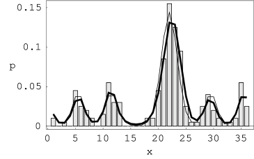
Figure 6: Gaussian prior with periodic reference potential and additional energy measurement, with initial guess $v^{(0)}$ different from that of Fig. 5. (Reference potential $v_{0}$ given in (108), energy penalty term as in (102) All parameters as for Fig. 5. Iterated with initial guess $v^{(0)}(x)$ = $v_{0}(x)$ for $0<x\leq 12,\,25\leq x$ and $v^{(0)}(x)$ = $0$ for $13\leq x\leq 24$.)

Including an additional noisy energy measurement (102) Fig. 5 shows that the depth of the potential is indeed better approximated than in Fig. 4. To avoid local maxima of the posterior the solution of Fig. 4 has been used as initial guess and the factor $\mu$ multiplying the average energy term has been slowly increased to its final value. Fig. 5 still only represents a local and no global maximum of the posterior, as can be by seen by starting with a different initial guess $v^{(0)}$. In Fig. 6 a better solution for the same parameters is presented where the initial guess has been selected using a priori information about the location of the impurity region.

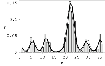
Figure 7: Approximate periodicity implemented by an inverse covariance ${\bf K}_{0}$ = $-\lambda(\Delta+\gamma\Delta_{\theta})$ as in Eq. (27). (With $\gamma$ = 1.0, $\lambda$ = 0.2, a fixed $\theta$ = 6, energy penalty term with $\mu$ = 1000, and zero reference potential $v_{0}\equiv 0$. Initial guess $v^{(0)}$ = $v_{0}\equiv 0$. All other parameters as for Fig. 4. )

Alternatively to a Gaussian prior with periodic reference, approximate periodicity can be enforced by the inverse covariance of a Gaussian prior. In this case the prior favors periodicity but no special form of the potential. The prior is thus less specific than a prior with explicit periodic reference function. Corresponding BIQM results for the inverse covariance (27) are shown in Fig. 7. Indeed while the potential is well approximated in regions where many observations have been collected, it is not as well approximated in regions where no or only few data are available. These are the regions where the prior dominates the observational data. In particular, in the case presented in Fig. 7, the zero reference function $v_{0}\equiv 0$ of an additional Laplacian smoothness prior implements a tendency to flat potentials.

If impurities are expected, a prior with one fixed periodic reference potential for the whole region is no adequate choice. Near impurities one would like to switch off the standard periodic reference potential which in these regions will be misleading. Because it is usually not known in advance where a given reference should be used and where not, those regions must be identified during learning. As first example we study a prior energy similar to Eq. (63),

$$E(v) = \frac{\lambda_{1}}{2}\int\!dx\,|v(x)-v_{0}(x)|^{2}[1-B(x)]-\frac{\lambda_{2}}{2}\langle v\,|\,\Delta\,|\,v\rangle,$$

which allows to switch off a given reference locally by means of a binary switching function defined as $B(x)$ = $\Theta\left(|v(x)-v_{0}(x)|^{2}-\vartheta\right)$. (An average energy term $E_{U}$ = $\frac{\mu}{2}(U-\kappa)^{2}$ could easily be included.) In the prior energy (LABEL:eq1) the reference $v_{0}$ is only used if $|v(x)-v_{0}(x)|^{2}$ is smaller than the given threshold $\vartheta$. Starting with a smoothed version of Eq. (LABEL:eq1) with a real mixing function $B(x)$ = $\sigma\left(|v(x)-v_{0}(x)|^{2}-\vartheta\right)$, the results of Fig. 8 have been obtained by changing during iteration $\sigma(x)$ slowly from a sigmoid to a step function. Using a step function for $B$ directly from the beginning leads to nearly indistinguishable results. Compared to Fig. 7 the reconstruction in Fig. 8 is improved mainly in the unperturbed region where the algorithm can now use the correct reference potential. An additional advantage is that the final auxiliary field $B(x)$ directly shows the identified impurity regions. One sees in Fig. 8 that the auxiliary field $B(x)$ is always switched off if the solution $v(x)$ is similar enough to the template $v_{0}(x)$.

The two $v$–dependent terms in Eq. (LABEL:eq1) can be combined [compare Eqs. (63) and (64)]. Skipping a term which only depends on $v$ through $B(x)$, one arrives at another prior which also implements local switching. More general, choosing the prior energy (76) for switching between two filtered differences with two reference potentials $v_{1}$ and $v_{2}$ leads to

$$E(v) = \frac{\lambda_{1}}{2}\int\!dx\,[1-B(x)]|\omega_{1}(x)|^{2}$$ (111)

$$+\frac{\lambda_{2}}{2}\int\!dx\,B(x)|\omega_{2}(x)|^{2},$$

where the switching is controlled by the binary function $B(x)$ = $\Theta\left(|\omega_{1}(x)|^{2}-|\omega_{2}(x)|^{2}-\vartheta\right)$ defined in terms of the filtered differences $\omega_{i}(x)$ = $(\partial/\partial x)[v(x)-v_{i}(x)]$. A prior energy (111) with two different nonzero reference potentials $v_{1}$ and $v_{2}$ is obtained, for example, when a different nonzero reference potential is given for the unperturbed and the perturbed region. The number of changes in the switching function $B(x)$ = $\Theta\left(|\omega_{1}(x)|^{2}-|\omega_{2}(x)|^{2}-\vartheta\right)$, can be controlled by adding a prior term $p(B)$ penalizing the number of times the function $B(x)$ changes its value. To avoid local minima for binary $B(x)$, simulated annealing techniques are useful. We have obtained an initial guess for $v$, and thus for $B(x)$, by writing $v(x)$ = $[1-c(x)]v_{1}(x)+c(x)v_{2}(x)$ and optimizing the binary function $c(x)$ by simulated annealing with respect to the likelihood and the additional prior $p(B)$. In particular, starting from $c(x)$ = $0$, new trial functions have been generated by selecting two points $x_{1}$, $x_{2}$ randomly and exchanging the function values zero and one in between (see Fig. 2). A new trial function has been accepted or rejected using the Metropolis rule $p($accept) = min$[1,\exp({-\beta_{\rm ann}\Delta E_{\rm ann}})]$ with $\Delta E_{\rm ann}$ denoting the difference in the error between actual function and new trial function. In the present case we have $E_{\rm ann}(v)$ = $\sum_{i}E(x_{i}|\hat{x},v)$ + $E_{B}(v)$ where $E(x_{i}|\hat{x},v)$ = $-\ln p(x_{i}|\hat{x},v)$ and $p(B)\propto\exp(-E_{B})$. The annealing temperature $1/\beta_{\rm ann}$ decreases during optimization.

Fig. 9 shows the reconstruction results using the following two reference potentials

$$v_{1}(x) = \frac{2}{3}\sin\left(\frac{2\pi}{6}x\right),$$ (112)

$$v_{2}(x) = \sin^{2}\left(\frac{2\pi}{6}x\right){\rm sign}\left[\sin\left(\frac{2\pi}{6}x\right)\right].$$ (113)

Compared to Fig. 8 the reconstruction is improved in the perturbed region, where the algorithm can now rely on a useful reference potential.

Finally, the switching function can be introduced as local hyperfield. As an example for a prior with hyperfield, Fig. 10 shows the reconstruction with the prior energy

$$E(v,\theta)=\frac{\lambda_{1}}{2}\mbox{$\langle v-v_{0}(\theta)\,|\,v-v_{0}(\theta)\rangle$}-\frac{\lambda_{2}}{2}\langle v\,|\,\Delta\,|\,v\rangle-\ln p(\theta),$$ (114)

where $v_{0}(x;\theta)$ = $v_{1}(x)[1-\theta(x)]+v_{2}(x)\theta(x)$ with the reference potentials of Eq. (112) and Eq. (113). A hyperprior $p(\theta)$ has been used penalizing the number of discontinuities of the hyperfield $\theta(x)$, analogous to $p(B)$ for Fig. 9. The $E(v|\theta)$ part of the prior energy (114) is of the form (49) with $\theta$–independent covariances. Hence the $\theta$–independent normalization factor can be skipped. An initial guess for the local hyperfield $\theta(x)$ has been obtained by simulated annealing as described for Fig. 9. As in this case optimization is required only with respect to the $\theta$–dependent parts of the posterior, optimizing $\theta(x)$ for given $v$ is faster than optimizing $v$ through $c(x)$ which requires diagonalization of the hamiltonian $H$ for every new trial function. However, as $\theta(x)$ is independent of $v$, the hyperfield has to be updated during iteration which has also been done by simulated annealing. As expected, a reconstruction with the non–Gaussian prior corresponding to the prior energy (111) is very similar to a reconstruction using hyperfields as in Eq. (114).

Figure 2: Generation of new trial configurations for simulated annealing by selecting two points randomly and exchanging the values zero and one of the binary function in between. This mechanism has been used to optimize the binary functions $c(x)$ and $\theta(x)$.

7 Conclusion

A nonparametric Bayesian approach has been developed and applied to the inverse problem of reconstructing potentials of quantum systems from observational data. Relying on observational data only the problem is typically ill–defined. It is therefore essential to include adequate a priori information. Since reconstructed potentials obtained by Bayesian Inverse Quantum Mechanics (BIQM) depend sensitively on the implemented a priori information, flexible prior models are required which can be adapted to the specific situation under study. In particular, the use of hyperparameters, hyperfields, and non–Gaussian priors with auxiliary fields has been discussed in detail. In this paper we have focussed on the implementation of approximate periodicity for potentials in inverse problems of quantum statistics. The presented prior models, however, can be useful for many empirical learning problems, including for example regression or general density estimation. Several variants of implementing a priori information on approximate periodicity have been tested and compared numerically.

Figure 3: Gaussian prior with Laplacian inverse covariance, zero reference potential, and additional noisy energy measurement. Top: Empirical density $p_{\rm emp}$ (bars), true likelihood $p_{\rm true}$ (thin), reconstructed likelihood $p_{\rm BIQM}$ (thick) Bottom: Reconstructed potential $v_{\rm BIQM}$ (thick) and true potential $v_{\rm true}$ (thin). (With 200 data points, $m$ = 0.25 for $\hbar$ = 1, $\beta$ = 4. Gaussian prior (11) with inverse covariance ${\bf K}_{0}$ = $-\lambda\Delta$, $\lambda$ = 0.2, zero reference potential $v_{0}\equiv 0$, and an additional energy penalty term of the form (102) with $\mu$ = 1000 and $\kappa$ = $-0.330$, equal to the true average energy $U(v_{\rm true})$. The solution has been obtained by iterating according to Eq. (105) with ${\bf A}$ = ${\bf K}_{0}$, starting with initial guess $v^{(0)}\equiv 0$. The optimal step width $\eta$ has been determined for each iteration by a line search algorithm.)

Figure 4: Gaussian prior with periodic reference potential without noisy energy measurement. Top: Empirical density $p_{\rm emp}$ (bars), true likelihood $p_{\rm true}$ (thin), reconstructed likelihood $p_{\rm BIQM}$ (thick) Bottom: Reconstructed potential $v_{\rm BIQM}$ (thick). true potential $v_{\rm true}$ (thin), and reference potential $v_{0}$ (dashed) of Eq. (108). (Number of data points and parameters $m$, $\beta$, ${\bf K}_{0}$, and $\lambda$ as for Fig. 3 but with $\mu$ = 0. The solution has been obtained by iterating according to (105) as described for Fig.3 with initial guess $v^{(0)}=v_{0}$.)

Figure 5: Gaussian prior with periodic reference potential and additional energy measurement, improving the approximation of the minima. (Reference potential $v_{0}$ given in (108), energy penalty term as in (102) with $\mu$ = 1000 and $\kappa$ = $-0.330$. All other parameters as for Fig. 4. Iterated with the solution shown in Fig. 4 as initial guess $v^{(0)}$.)

Figure 8: Local switching between periodic and zero reference potential. The black bars on top indicate regions where $B(x)$ = 1, i.e., regions where impurities have been identified. (Prior of Eq. (LABEL:eq1) with $\lambda_{1}$ = 0.2, $\lambda_{2}$ = 0.2, $\mu$ = 0, and reference potential as in (108). The $v$–dependent function $B(x)$ was slowly changed from a sigmoid to a step function during iteration, keeping the threshold $\vartheta$ = $0.15$ fixed. All other parameters as in Fig. 4. Initial guess $v^{(0)}$ as for Fig. 6)

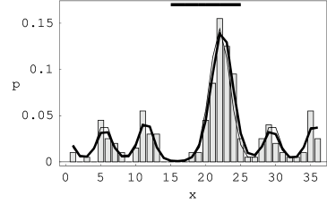
Figure 9: Local switching between two nonzero reference potentials. (Reference potentials $v_{1}$, $v_{2}$ given in (112) and (113). Prior of Eq. (111), with $\lambda_{1}$ = $\lambda_{2}$ = 10, $\mu$ = 0. Step function for $B(x)$ with $\vartheta$ = 0. An additional prior $p(B)$ on $B$ has been included with $-\ln p(B)/10$ counting the number of discontinuities of the function $B(x)$. Other parameters as in Fig. 4.)

Figure 10: Prior with local hyperfield. (Prior of Eq. (114), with $\lambda_{1}$ = 10, $\lambda_{2}$ = 1, $\vartheta$ = 0, $\mu$ = 0, including a hyperprior $p(\theta)$ with $E_{B}/10$ counting the number of discontinuities of the hyperfield $\theta(x)$. Other parameters as in Fig. 4.)

References

- (1) A.N. Tikhonov, V. Arsenin, Solution of Ill–posed Problems. (New York: Wiley, 1977).
- (2) A. Kirsch, An Introduction to the Mathematical Theory of Inverse Problems. (New York: Springer Verlag, 1996).
- (3) V.N. Vapnik, Statistical Learning Theory. (New York: Wiley, 1998).
- (4) J. Honerkamp, Statistical Physics. (New York: Springer Verlag, 1998)
- (5) R.G. Newton, Inverse Schrödinger Scattering in Three Dimensions. (New York: Springer Verlag, 1989).
- (6) K. Chadan, P.C. Sabatier, Inverse Problems in Quantum Scattering Theory. (Berlin: Springer Verlag, 1989)
- (7) K. Chadan, D. Colton, L. Päivärinta, W. Rundell, An Introduction to Inverse Scattering and Inverse Spectral Problems. (Philadelphia: SIAM, 1997).
- (8) I.M. Gel’fand, B.M. Levitan, Trans. Amer. Soc. 1, 253–302 (1951).
- (9) M. Kac, Can one hear the shape of a drum? Am. Math. Mon. 73, 1–23 (1966).
- (10) V.A. Marchenko, Sturm–Liouville Operators and Applications. (Basel: Birkhäuser, 1986).
- (11) B.N. Zakhariev, V.M. Chabanov, Inverse Problems 13, R47–R79 (1997).
- (12) J.C. Lemm, J. Uhlig, A. Weiguny, Phys. Rev. Lett. 84, 2068 (2000).
- (13) J.C. Lemm, Bayesian Field Theory. Technical Report No. MS-TP1-99-1, Univ. of Münster, arXiv:physics/9912005, (1999).
-
(14)
J.C. Lemm,
Inverse Time–Dependent Quantum Mechanics.
Technical Report, MS-TP1-00-1, Münster University,
arXiv:quant-ph/0002010, (2000). - (15) J.C. Lemm, J. Uhlig, Phys. Rev. Lett. 84, 4517 (2000)
- (16) C.W. Helstrom, Quantum Detection and Estimation Theory. (New York: Academic Press, 1976).
- (17) A.S. Holevo, Probabilistic and Statistical Aspects of Quantum Theory. (Amsterdam: North–Holland, 1982).
- (18) M. Tan, J. Mod. Opt. 44 2233 (1997).
- (19) V. Buz̃ek, G. Drobný, R. Derka, G. Adam, H. Wiedemann, arXiv:quant-ph/9805020.
- (20) T.R. Bayes, Phil. Trans. Roy. Soc. London 53, 370 (1763), reprinted in Biometrika 45, 293 (1958).
- (21) J.O. Berger, Statistical Decision Theory and Bayesian Analysis. (New York: Springer Verlag, 1980).
- (22) T. Loredo, From Laplace to Supernova SN 1987A: Bayesian Inference in Astrophysics. In Fougère, P.F. (ed.) Maximum-Entropy and Bayesian Methods, Dartmouth, 1989, 81–142. (Dordrecht: Kluwer, 1990), available at http://bayes.wustl.edu/gregory/gregory.html.
- (23) J.M. Bernado, A.F. Smith, Bayesian Theory. (New York: John Wiley, 1994).
- (24) A. Gelman, J.B. Carlin, H.S. Stern, D.B. Rubin, Bayesian Data Analysis. (New York: Chapman & Hall, 1995).
- (25) D.S. Sivia, Data Analysis: A Bayesian Tutorial. (Oxford: Oxford University Press, 1996).
- (26) B.P. Carlin, T.A. Louis, Bayes and Empirical Bayes Methods for Data Analysis. (Boca Raton: Chapman & Hall/CRC, 1996).
- (27) N. Metropolis, A.W. Rosenbluth, M.N. Rosenbluth, A.H. Teller, E. Teller, Journal of Chemical Physics 21, 1087–1092, (1953).
- (28) K. Binder, D.W. Heermann, Monte Carlo simulation in statistical physics: an introduction. (Berlin: Springer Verlag, 1988).
- (29) R.M. Neal, Monte Carlo Implementation of Gaussian Process Models for Bayesian Regression and Classification. Technical Report No. 9702, Dept. of Statistics, Univ. of Toronto, Canada (1997).
- (30) N.G. De Bruijn, Asymptotic Methods in Analysis. (New York: Dover, 1981), originally published in 1958 by the North–Holland Publishing Co., Amsterdam.
- (31) N. Bleistein, N. Handelsman, Asymptotic Expansions of Integrals. (New York: Dover 1986), originally published in 1975 by Holt, Rinehart and Winston, New York.
- (32) F. Girosi, M. Jones, T. Poggio, Neural Computation 7 (2), 219–269 (1995).
- (33) J.C. Lemm, Prior Information and Generalized Questions. A.I.Memo No. 1598, C.B.C.L. Paper No. 141, Massachusetts Institute of Technology, (1996), available at http://pauli.uni-muenster.de/∼lemm.
- (34) J.C. Lemm, How to Implement A Priori Information: A Statistical Mechanics Approach. Technical Report MS-TP1-98-12, Münster University, arXiv:cond-mat/9808039 (1998).
- (35) C.M. Bishop, Neural Networks for Pattern Recognition. (Oxford: Oxford University Press, 1995).
- (36) J.C. Lemm, Mixtures of Gaussian Process Priors. In Proceedings of ICANN 99 IEEE Conference Publication, Vol. 1, pp 292–297 (London, IEEE, 1999).
- (37) J.H. Holland, Adaption in Natural and Artificial Systems. (University of Michigan Press, 1975), 2nd ed. MIT Press, 1992.
- (38) D.E. Goldberg, Genetic Algorithms in Search, Optimization, and Machine Learning. (Redwood City, CA: Addison–Wesley, 1989).
- (39) Z. Michalewicz, Genetic Algorithms + Data Structures = Evolution Programs. (Berlin: Springer Verlag, 1992).
- (40) H.–P. Schwefel, Evolution and Optimum Seeking. (New York: Wiley, 1995).
- (41) M. Mitchell, An Introduction to Genetic Algorithms. (Cambridge, MA: MIT Press, 1996).
- (42) S. Kirkpatrick, C.D. Gelatt Jr., M.P. Vecchi, Science 220, 671–680 (1983).
- (43) M. Mezard, G. Parisi, M.A. Virasoro, Spin Glass Theory and Beyond. (Singapore: World Scientific, 1987).
- (44) E. Aarts, J. Korts, Simulated Annealing and Boltzmann Machines. (New York: Wiley, 1989).
- (45) S.B. Gelfand, S.K. Mitter, Algorithmica 6 (3) 419-436 (1991).
- (46) A.L. Yuille, J.J. Kosowski, Neural Computation 6 (3), 341–356 (1994).
- (47) S. Geman, D. Geman, Stochastic relaxation, Gibbs distributions and the Bayesian restoration of images. IEEE Trans. on Pattern Analysis and Machine Intelligence 6, 721–741 (1984), reprinted in Shafer & Pearl (eds.) Readings in Uncertainty Reasoning. (San Mateo, CA: Morgan Kaufmann, 1990)
- (48) T. Poggio, V. Torre, C. Koch, Computational vision and regularization theory. Nature 317, 314–319, (1985).
- (49) J.L. Marroquin, S. Mitter, T. Poggio, J. Am. Stat. Assoc. 82, 76–89 (1987).
- (50) D. Geiger, F. Girosi, IEEE Trans. on Pattern Analysis and Machine Intelligence 13 (5), 401–412 (1991).
- (51) S.C. Zhu, A.L. Yuille, IEEE Trans. on Pattern Analysis and Machine Intelligence 18 (9), 884–900 (1996).
- (52) T. Roths, D. Maier, Chr. Friedrich, M. Marth, J. Honerkamp, Rheol. Acta 39 (2) 163-173 (2000).
- (53) G. Winkler, Image Analysis, Random Fields and Dynamic Monte Carlo Methods. (Berlin: Springer Verlag, 1995).
- (54) S.C. Zhu, D. Mumford, IEEE Trans. on Pattern Analysis and Machine Intelligence 19 (11), 1236–1250 (1997).
- (55) S.C. Zhu, Y.N. Wu, D. Mumford, Neural Computation, 9 (8), 1627–1660 (1997).
- (56) W.H. Press, S.A. Teukolsky, W.T. Vetterling, B.P. Flannery, Numerical Recipes in C. (Cambridge: Cambridge University Press, 1992).
- (57) W. Zhu, H. Rabitz, J. Chem. Phys. 111, 472–480 (1999).