Interference at quantum transitions: lasing without inversion and resonant four-wave mixing in strong fields at Doppler-broadened transitions

Abstract

An influence of nonlinear interference processes at quantum transitions under strong resonance electromagnetic fields on absorption, amplification and refractive indices as well as on four-wave mixing processes is investigated. Doppler broadening of the coupled transitions, incoherent excitation, relaxation processes, as well as power saturation processes associated with the coupled levels are taken into account. Both closed (ground state is involved) and open (only excited states are involved) energy level configurations are considered. Common expressions are obtained which allow one to analyze the optical characteristics (including gain without inversion and enhanced refractive index at vanishing absorption) for various $V$, $\Lambda$ and $H$ configurations of interfering transitions by a simple substitution of parameters. Similar expressions for resonant four-wave mixing in Raman configurations are derived too. Crucial role of Doppler broadening is shown. The theory is applied to numerical analysis of some recent and potential experiments.

Keywords: quantum interference, lasing without inversion, resonant four-wave mixing, Doppler and strong field effects. PACS: 42.50.Gy, 42.55.-f, 42.65

I INTRODUCTION

Many concepts of quantum optics were originated proceeding from the assumed equality of probabilities of induced transitions accompanied by an absorption and emission of photons predicted by A. Einstein. Requirement of population inversion for lasing is direct consequence from this equality.

At the presence of several resonant electromagnetic fields, probability amplitudes of a coupled quantum states contain several oscillating components at close frequencies. Therefore alongside with squared modules of appropriate components cross terms indicating an interference of quantum transitions appear while calculating transitions probabilities. The coherent nonlinear optical phenomena stipulated by the indicated evolution of quantum states, driven by several fields, were called as nonlinear interference effects ($NIE$) [1, 2]. In quantum optics $NIE$ may result in different coupling of a radiation with atoms in absorbing and emitting states controlled by the auxiliary fields [3, 4]. Various appearances of these effects are feasible. Soon after discovery of lasers Rautian and Sobelman [5] showed feasibility of amplification without inversion ($AWI$) in two-level systems. The features of $AWI$ in optical three-level systems were explored in [6, 2]. Studies of $NIE$ in absorption/gain spectra including experiments on generation of an optical radiation in three-level systems, so that generation was possible only at the expense of nonlinear interference effects, drew much attention in 60th and 70th [7]. (Review of relevant optical experiments and of earlier papers on $AWI$ in microwave range see in [9, 8].) Coherent population trapping ($CPT$) is one of the appearances of $NIE$ for the states with negligible relaxation rates and Doppler effects. In 80th – 90th studies of coherent interference processes at quantum transitions have been attracting much interest again in the context of $AWI$, electromagnetically - induced transparency ($EIT$), $CPT$, enhanced nonlinear optical frequency conversion and other manifestations of these effects [10].

In classical terms an emission and absorption of a radiation are stipulated by forced oscillations of bound charges and depend on phase difference between radiation and induced oscillations. However, a radiation may simultaneously drive several coherent interfering oscillations of a various origin. Depending on a relation of their phases and amplitudes the interference can be either constructive or destructive, full or partial. Thus the matching components of an optical response can either amplify or suppress each other. On the other hand, the macroscopic response of a medium can be thought as result of quantum transitions, at which the photons can

11th International Vavilov Conference on Nonlinear Optics, 24-28 June 1997, Novosibirsk, Russia SPIE Vol. 3485

simultaneously contribute in several quantum pathways. By applying semi-classical approach a deep analogy with many well known effects of classical physics can be used to interpret and foresee the relevant quantum optics effects. Thus, leaving aside classifications of involved elementary quantum processes (introduced and valid for weak fields in the limits of perturbation theory), it is possible to predict and to explain wide range of optical processes, stipulated by quantum interference, some of them are quite unusual.

The objective of the paper is to consider various appearance of interference effects in resonance nonlinear - optical processes with the aid of the outlined approach in a context of some recent experiments. The amplitude and phase relations of interfering intra-atomic oscillations depend on configuration and on relaxation characteristics of the coupled transitions, on type of nonlinear-optical process, on intensities and frequency detunings of the radiations from resonances. Due to the difference in Doppler shifts the contributions to the macroscopic polarization of atoms at various velocities in gases may interfere in a different way too. The interference appears differently in an absorption, refraction and in different four-wave mixing ($FWM$) processes.

As an illustration of $NIE$ the following results will be presented:

1. The possibility of an amplification of a radiation without inversion of saturated populations on resonant transition is investigated. Influence of the growth of intensity of an amplified radiation on inversionless amplification in various open and closed transition configurations is analyzed. The conditions are formulated and with the concrete examples is shown, that by proper change of incoherent excitation rate of levels and of auxiliary radiation intensity the index of an inversionless amplification does not decrease with growth of intensity of an amplified radiation. The elements of the theory of such lasing without inversion are presented.

2. It is shown, that due to Maxwell velocity distribution of atoms and corresponding inhomogeneous broadening of the coupled transitions, incoherent excitation of the intermediate levels may drastically change both spectral properties and a magnitude (by orders of magnitude) of nonlinear susceptibilities for resonant $FWM$ processes. As the consequence, important power saturation effects appear. These features must be taken into account for explanation of the experiments and optimization of frequency-conversion. Resonant $FWM$ coupling of two strong and two weak radiations is considered. Formulas for both cases of coupling, one is relevant to coherent population trapping, another – when each level is coupled to only one driving field are derived. The outcomes are applied to numerical analysis and to discussion of recent experiments [11].

II ABSORPTION AND REFRACTION INDICES FOR A STRONG RADIATION AT THE PRESENCE OF OTHER STRONG RADIATION, COUPLED TO AN ADJACENT TRANSITION

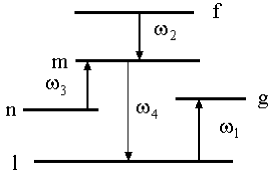
FIG. 1: Transition configurations.

First, consider interaction of two strong laser fields at the three-level system. Possible configurations of such systems are shown in FIG.1: folded $V$ and $\Lambda$, and cascade - $H$. In further we shall investigate spectral features of a gas material for a radiation $E_{4}$ at frequency $\omega_{4}$, tunable in the vicinity of a transition $l-m$. It’s intensity is not supposed weak. Depending on the configuration of transitions under consideration one of the auxiliary strong fields $E_{1}$, $E_{3}$ or $E_{2}$ with frequencies $\omega_{1}$, $\omega_{3}$, $\omega_{2}$, resonant to adjacent transitions shown in the figure is turned on. All radiations are supposed to be uniformly polarized co- or counter-propagating travelling wave: $E_{j}(z,t)=E_{j}\exp\{-[i(\omega_{j}t-k_{j}z)]\}+k.c.,$ where $k_{j}$ - can take both positive and negative values, $j=1,2,3,4$. Incoherent excitation of the levels with Maxwell’s velocity distribution, all possible population and coherence relaxation channels are accounted for.

It is necessary to distinguish the open and closed energy-level configurations. In open one (lowest level is not ground), the rate of incoherent excitation of the levels by an external source practically does not depend on the rate of induced transitions between considered levels. In the closed one (lowest level is ground one), the excitation rate for atoms at different levels and velocities depends on the value and velocity distribution of the other populations, which are dependent on the intensity of the driving fields.

A General equations for absorption end refraction indices

Power dependent susceptibility $\chi_{4}$, responsible for absorption and refraction, can be found from the equation:

$$P^{NL}(\omega_{4})=N\chi_{4}E_{4},$$ (1)

where polarization $P^{NL}(\omega_{4})$ is convenient to calculate with aid of density matrix $\rho_{ij}$:

$${P}=N\rho_{ij}d_{ji}+{c.c.}.$$ (2)

Taking into account above discussed relaxation and incoherent excitation processes, density matrix equations for a mixture of pure quantum mechanical ensembles in the interaction representation can be written in general form as:

$$L_{nn}\rho_{nn}=q_{n}-i[V,\rho]_{nn}+\gamma_{mn}\rho_{mm},L_{lm}\rho_{lm}=L_{4}\rho_{4}=-i[V,\rho]_{lm},$$ (3)

$$L_{ij}=d/dt\,+\Gamma_{ij},\quad V_{lm}=G_{lm}\cdot\exp\{i[\Omega_{4}t-kz]\},\quad G_{lm}=-{\bf E_{4}\cdot d_{lm}}/2\hbar,$$

where $\Omega_{4}=\omega_{4}-\omega_{mn}$ - frequency detuning from resonance; $\Gamma_{mn}$ - homogeneous half-widths of transitions, in absence of collisions $\Gamma_{mn}=(\Gamma_{m}+\Gamma_{n})/2$; $\Gamma_{n}=\sum_{j}\gamma_{nj}$ - inverse lifetimes of levels; $\gamma_{mn}$ - rate of relaxation from the level $m$ to $n$, $q_{n}=\sum_{j}w_{nj}r_{j}$ - rate of incoherent excitation to a state $n$ from underlying levels. For open configurations $q_{i}$ - is mainly determined by the population of the ground state and practically does not depend on the driving fields.

In a steady-state regime a set of density-matrix equation may be reduced to the set of algebraic equations [12]. Below we present only results of calculations. Despite of essential distinctions in manifestations of $NIE$ in different open and closed configuration, formulas for absorption/gain ($\alpha$) and resonant part of refractive ($\delta n$) indices and also for power dependent populations of the levels can be presented uniformly for all configurations shown on FIG.1:

$$\alpha_{4}/\alpha_{04}=Re\{\chi_{4}/\chi_{4}^{0}\},\>\delta n_{4}/2\delta n_{04}=Im\{\chi_{4}/\chi_{4}^{0}\},\>\alpha_{i}/\alpha_{0i}=Re\{\chi_{i}/\chi_{i}^{0}\},\>\delta n_{i}/2\delta n_{0i}=Im\{\chi_{i}/\chi_{i}^{0}\},$$

$$\dfrac{\chi_{4}}{\chi_{4}^{0}}=\dfrac{\Gamma_{4}}{P_{4}}\dfrac{\Delta r_{4}(1+u_{2})\mp\Delta r_{i}g_{2}}{\Delta n_{4}(1+g_{1}+u_{2})},\qquad\dfrac{\chi_{i}}{\chi_{i}^{0}}=\dfrac{\Gamma_{i}}{P_{i}}\dfrac{\Delta r_{i}(1+g_{1}^{*})\mp\Delta r_{4}u_{1}^{*}}{\Delta n_{4}(1+g_{1}^{*}+u_{2}^{*})},$$ (4)

Here and further index $i$ specifies transition, resonant to the auxiliary radiation (see FIG.1), $\chi$ is susceptibility, $\alpha_{0},\delta n_{0},\chi_{0}$ are corresponding maximum resonant values at zero field intensities, $P_{j}=\Gamma_{j}+i\Omega_{j}$ (for example: $P_{lm}=P_{4}=\Gamma_{4}+i\Omega_{4}$, $P_{lm}=P_{ml}^{*}$, $P_{lf}=P_{42}=\Gamma_{lf}+i(\Omega_{4}+\Omega_{2})$ etc.). If the atom moves with speed $v$, Doppler shift of resonances must be taken into account by substitution $\Omega_{j}$ for $\Omega_{j}^{{}^{\prime}}=\Omega_{j}-k_{j}v$. In further strokes will be omitted, but it is supposed, that the Doppler shift in the formulas is taken into account. $\Delta r_{4}=r_{l}-r_{m}$ is power dependent population difference; $\Delta n_{4}=n_{l}-n_{m}$, $n_{i}$ - population of the level in absence of driving fields, which is described by the formula: $n_{i}=(q_{i}/\Gamma_{i})+(\gamma_{ki}/{\Gamma_{i}})({q_{k}}/{\Gamma_{k}})$.

$$g_{1}={|G_{i}|^{2}}/{P_{4}P_{4i}},g_{2}={|G_{i}|^{2}}/{P_{i}^{*}P_{4i}},u_{1}={|G_{4}|^{2}}/{P_{4}P_{4i}},u_{2}={|G_{4}|^{2}}/{P_{i}^{*}P_{4i}}.$$ (5)

$G_{j}$ are coupling Rabi frequencies. Formulas for populations differences can be presented uniformly too:

$$\Delta r_{4}=(\Delta n_{4}X_{2}\mp\Delta n_{i}X_{3})/(X_{1}X_{2}-X_{3}X_{4}),\Delta r_{i}=(\Delta n_{i}X_{1}\mp\Delta n_{4}X_{4})/(X_{1}X_{2}-X_{3}X_{4}).$$ (6)

$$X_{2}=1+Re\{a_{24}\hbox{\ae}_{4}\dfrac{\Gamma_{4}}{P_{4}}\dfrac{g_{2}}{1+g_{1}+u_{2}}+a_{2i}\hbox{\ae}_{i}\dfrac{\Gamma_{i}}{P_{i}}\dfrac{1+g_{1}^{*}}{1+g_{1}^{*}+u_{2}^{*}}\},$$

$$X_{3}=Re\{a_{34}\hbox{\ae}_{4}\dfrac{\Gamma_{4}}{P_{4}}\dfrac{g_{2}}{1+g_{1}+u_{2}}+a_{3i}\hbox{\ae}_{i}\dfrac{\Gamma_{i}}{P_{i}}\dfrac{1+g_{1}^{*}}{1+g_{1}^{*}+u_{2}^{*}}\},$$

$$X_{1}=1+Re\{a_{14}\hbox{\ae}_{4}\dfrac{\Gamma_{4}}{P_{4}}\dfrac{1+u_{2}}{1+g_{1}+u_{2}}+a_{1i}\hbox{\ae}_{i}\dfrac{\Gamma_{i}}{P_{i}}\dfrac{u_{1}^{*}}{1+g_{1}^{*}+u_{2}^{*}}\},$$

$$X_{4}=Re\{a_{44}\hbox{\ae}_{4}\dfrac{\Gamma_{4}}{P_{4}}\dfrac{1+u_{2}}{1+g_{1}+u_{2}}+a_{4i}\hbox{\ae}_{i}\dfrac{\Gamma_{i}}{P_{i}}\dfrac{u_{1}^{*}}{1+g_{1}^{*}+u_{2}^{*}}\},$$

$$a_{14}=-a_{34},a_{1i}=-a_{3i},a_{24}=-a_{44},a_{2i}=-a_{4i}.$$ (7)

Sign minus in (A),(6) concerns to folded $V$ ($E_{4},E_{1}$) and $\Lambda$ ($E_{4},E_{3}$) schemes, plus - to cascade $H$ ($E_{4},E_{2}$) scheme. Beside that in the ladder $H$-scheme, $P_{i}$ must be substituted for $P_{i}^{*}$, and vice a versa: $P_{i}^{*}$ for $P_{i}$. $\hbox{\ae}_{4}$ and $\hbox{\ae}_{i}$ - are saturation parameters accordingly for transitions $4$ and $i$. For open configurations

$$\hbox{\ae}_{4}={2|G_{4}|^{2}(\Gamma_{l}+\Gamma_{m}-\gamma_{4})}/{(\Gamma_{l}\Gamma_{m}\Gamma_{4})},$$ (8)

whereas $\hbox{\ae}_{i}$ and parameters $a_{ij}$ depending only on relaxation constants are defined below for each configuration.

1. $V$ - scheme (fields $E_{4}$, $E_{1}$; $i=1$)

OPEN CONFIGURATION

$$\hbox{\ae}_{i}=\hbox{\ae}_{1}=\dfrac{2|G_{1}|^{2}(\Gamma_{g}+\Gamma_{l}-\gamma_{1})}{\Gamma_{g}\Gamma_{l}\Gamma_{1}},a_{2i}=a_{21}=1,a_{14}=1,a_{3i}=a_{31}=\dfrac{\Gamma_{g}-\gamma_{1}}{\Gamma_{g}+\Gamma_{l}-\gamma_{1}},a_{44}=\dfrac{\Gamma_{m}-\gamma_{4}}{\Gamma_{l}+\Gamma_{m}-\gamma_{4}}.$$ (9)

CLOSED CONFIGURATION

$$\hbox{\ae}_{4}={4|G_{4}|^{2}}/{\Gamma_{m}\Gamma_{4}},\hbox{\ae}_{i}=\hbox{\ae}_{1}={4|G_{1}|^{2}}/{\Gamma_{g}\Gamma_{1}},$$

$$a_{3i}=a_{31}=0.5\Delta n_{4},a_{44}=0.5\Delta n_{1},a_{2i}=a_{21}=0.5[1+\Delta n_{1}],a_{14}=0.5[1+\Delta n_{4}].$$ (10)

2. $\Lambda$ - scheme (fields $E_{4}$, $E_{3}$, $i=3$)

OPEN CONFIGURATION

$$\hbox{\ae}_{3}={2|G_{3}|^{2}(\Gamma_{m}+\Gamma_{n}-\gamma_{3})}/{\Gamma_{m}\Gamma_{n}\Gamma_{3}},\quad a_{2i}=a_{23}=1,\quad a_{14}=1,$$

$$a_{3i}=a_{33}={\Gamma_{n}}{(\Gamma_{l}-\gamma_{4})}/{\Gamma_{l}}{(\Gamma_{m}+\Gamma_{n}-\gamma_{3})},\quad a_{44}={\Gamma_{l}}{(\Gamma_{n}-\gamma_{3})}/{\Gamma_{n}}{(\Gamma_{m}+\Gamma_{l}-\gamma_{4})}.$$ (11)

CLOSED CONFIGURATION

$$\hbox{\ae}_{4}=\dfrac{4|G_{4}|^{2}}{\Gamma_{m}\Gamma_{4}},\quad a_{3i}=a_{33}=1+\Delta n_{4}-(1+2\Delta n_{4})\dfrac{\Gamma_{m}-\gamma_{3}}{\Gamma_{m}+\Gamma_{n}-\gamma_{3}},\ a_{44}=0.5[1-\dfrac{\gamma_{3}}{\Gamma_{n}}+\Delta n_{3}(1+\dfrac{\gamma_{3}}{\Gamma_{n}})],$$

$$a_{2i}=a_{23}=1+\Delta n_{3}(\Gamma_{n}-\Gamma_{m}+\gamma_{3})/(\Gamma_{n}+\Gamma_{m}-\gamma_{3}),\ a_{14}=0.5[1+\Delta n_{4}(1+\gamma_{3}/\Gamma_{n})].$$ (12)

H-scheme (fields $E_{4}$, $E_{2}$; $i=2$)

OPEN CONFIGURATION

$$\hbox{\ae}_{2}=\dfrac{2|G_{2}|^{2}(\Gamma_{f}+\Gamma_{m}-\gamma_{2})}{\Gamma_{f}\Gamma_{m}\Gamma_{2}};\ a_{14}=1;\quad a_{2i}=a_{22}=1;\ a_{3i}=a_{32}=\dfrac{\Gamma_{l}-\gamma_{4}}{\Gamma_{l}}\dfrac{\Gamma_{f}-\gamma_{2}}{\Gamma_{m}+\Gamma_{f}-\gamma_{2}};\ a_{44}=\dfrac{\Gamma_{l}}{\Gamma_{l}+\Gamma_{m}-\gamma_{4}}.$$ (13)

CLOSED CONFIGURATION

$$\hbox{\ae}_{4}={4|G_{4}|^{2}}/{\Gamma_{m}\Gamma_{4}},\ a_{3i}=a_{32}=(1+2\Delta n_{4})(\Gamma_{f}-\gamma_{2})/(\Gamma_{m}+\Gamma_{f}-\gamma_{2})-\Delta n_{4},\ a_{44}=0.5(1-\Delta n_{2}),$$

$$a_{14}=0.5(1+\Delta n_{4}),\ a_{2i}=a_{22}=1+\Delta n_{2}(\Gamma_{m}-\Gamma_{f}+\gamma_{2})/(\Gamma_{m}+\Gamma_{f}-\gamma_{2}).$$ (14)

$NIE$ are associated with coherence at two-photon transitions and disappear at $|P_{4i}|\rightarrow\infty$. At $G_{4}=0$ formulas (A), (6) converge into those, similar to discussed and analyzed in [6, 2, 8, 9]. Following [6], range of parameters where amplification is not accompanied by the inversion of power-dependent populations can be easily found from (A), (6). For the resonant coupling in $V$ and $\Lambda$ schemes conditions for AWI at the transitions 4 and $i$ take the form, correspondingly:

$${\Delta r_{4}}/{\Delta r_{i}}<{g_{2}}/{(1+u_{2})};\quad{\Delta r_{i}}/{\Delta r_{4}}<{u_{1}}/{(1+g_{1})}.$$ (15)

Similar formulas for $H$ schemes show, that on the contrary to the previous configurations, inversion of populations on the adjacent transition is required for $AWI$ in center of the resonance, or amplification under certain conditions arises in wings of a resonance. (More detail formulas and analysis are given in [12].

Threshold and output power of lasing without inversion can be found from the equation:

$$\alpha_{4}=T,$$ (16)

Where $T$ is loss of a radiation from a laser cavity per one pass, scaled to the unit of length of the amplifying medium. Thus, the derived expressions determine conditions and characteristics of inversionless generation too.

B Numerical analysis

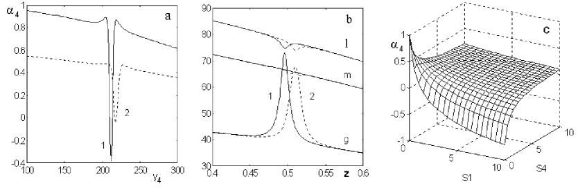
FIG. 2: Velocity-averaged absorption/gain index and populations vs velocities at inhomogeneously broadened $l-m$ transition ($l$ – excited state, open configuration) in the presence of strong field at $l-g$ transition ($Ne$, $2s_{2}$ – $2p_{4}$ – $3s_{2}$) (co-propagating waves). $\lambda_{1}=1150nm$, $\lambda_{4}=630nm$ ($Ne$), $\Gamma_{m}=3\cdot 10^{7}c^{-1}$, $\Gamma_{l}=5\cdot 10^{7}c^{-1}$, $\Gamma_{g}=10^{7}c^{-1}$, $\gamma_{ml}=\gamma_{ml}=0.5\cdot 10^{7}c^{-1}$. Ratio of initial populations is: $N_{l}:N_{g}:N_{m}=100:50:85$. a – absorption index ($y_{4}=\Omega_{4}/\Gamma_{lm}$), b – populations vs velocities ($z=v/\bar{v}$, frequency $\omega_{4}$ is locked to the absorption minimum). 1 – $S_{1}=|E_{1}d_{lg}/2\hbar|^{2}/\Gamma_{1}\Gamma_{gm}=5$, $S_{4}=|E_{4}d_{ml}/2\hbar|^{2}/\Gamma_{4}\Gamma_{gm}=0$. $\Omega_{1}=350\Gamma_{lg}$; 2 – $S_{1}=5$, $S_{4}=1$, $\Omega_{1}=360\Gamma_{lg}$. c – velocity-averaged absorption/gain index vs field intensities ($\Omega_{1}=\Omega_{4}=0$).

Below we shall apply the derived expressions for numerical analysis of $NIE$ in open ($Ne$) and closed ($Na$) configurations of transitions. The same transitions of $Ne$ were considered in [6] for illustration of possible AWI of weak probe field. The formulas for velocity averaged absorption index were derived and difference in $NIE$ for backward and forward waves in inhmogeneously broadened transitions was analyzed in [4, 2] for the cases of weak probe field and coupling Rabi frequency of driving field not exceeding Doppler width of the transition. Therefore in further main attention will be given to effects accompanying increase of intensity of an amplifying radiation.

FIG. 2a shows that inhomogeneous broadening does not destroy macroscopic coherence effects and $NIE$. The relative change of absorption index by an auxiliary field appears even larger, than for a homogeneously broadened transition. Coherent coupling gives rise to amplification at $\omega_{4}$ and establishes populations so that there is no inversion neither on one- nor on two-photon transitions FIG. 2b. With the growth of $E_{4}$ populations of $m$ and $g$ levels aim to equal magnitude, which indicates appearance of coherent population trapping. In the latter case a small modulation of velocity distribution on the level $m$ appears. Like in [6, 2], analysis shows that in order to attain $AWI$ certain ratio between initial (in the absence of the radiations) populations must be fulfilled. FIG. 2c shows that absorption (gain) strongly depends on the intensities of both driving and probe fields. As it was outlined, the open and closed systems differ both in possible magnitudes of relaxation parameters and in dependence of incoherent excitation on an intensity of the driving fields. FIG. 4 considers the case, when 36% of a ground state atoms are initially excited by an incoherent pump to a level $m$, that still may correspond to strong absorption at the transition $ml$. By that strong driving field $E_{1}$ may produce $AWI$ for co-propagating shorter-wavelength weak radiation at $\omega_{4}$, which makes approximately 50% from an initial absorption (FIG. 4a). The amplification happens in absence of saturated population inversion for all transitions (FIG. 4b). It is essential that a population of a top level $m$ depends on the strength of $E_{1}$ even at zero intensities of a probe radiation $E_{4}$.

FIG. 3: Velocity-averaged absorption - gain index (a) and populations vs velocities ($z=v/\bar{v}$) (b) at inhomogeneously broadened $l-m$ transition in the presence of strong field at $l-g$ transition ($l$ - ground state, closed configuration, co-propagating waves). $\lambda_{4}=330nm$, $\lambda_{1}=590nm$ ($Na$; $3P_{1/2}$ – $3S$ – $4P_{1/2}$). $\Gamma_{m}=9\cdot 10^{7}c^{-1}$, $\Gamma_{g}=63\cdot 10^{7}c^{-1}$, $N_{l}:N_{g}:N_{m}=64:0:36$. a: $1$ – $S_{1}=10,S_{4}=0,$ $y_{1}=0$;   $2$ – $S_{1}=10,S_{4}=20$, $y_{1}=20$. b – $\omega_{4}$ corresponds to: $1$ – to the right, $2$ – to the left point of a zero absorption of the appropriate curve in a .

FIG. 4: Velocity-averaged absorption/gain index vs field intensities for co-propagating waves ($\Omega_{1}=\Omega_{4}=0$). a – $N_{l}:N_{g}:N_{m}=64:0:36$; b – $N_{l}:N_{g}:N_{m}=60:0:40$. Other parameters are like in FIG. 4.

Curve 2 (FIG. 4a) shows, that the AWI strongly depend on intensity of an amplified radiation, that is accompanied for the given configuration by noticeable change of populations of levels $m$ and $l$. (FIG. 4b) displays energy and velocity distribution of the atoms corresponding to appearance of transparency at $\omega_{4}$. It is interesting to note that the distribution sharply varies with increase of intensity of $E_{1}$.

FIG. 4 shows, that $AWI$ may be maintained in a certain level with growth of intensity of an amplified radiation by changing incoherent excitation rate and strength of an auxiliary radiation.

III INTERFERENCE EFFECTS IN RESONANT $FWM$ AT DOPPLER BROADENED TRANSITIONS

The use of resonant $FWM$ in gases for frequency conversion allows one to decrease the required power of fundamental radiations down to the magnitudes characteristic for cw lasers [11, 13, 14, 15, 16]. $FWM$ concerns to so-called coherent nonlinear - optical processes, depending on phase-mismatch. As it was outline above, at resonant coupling, various coherent component stipulated by correlated quantum transitions and giving contribution to the process of radiation conversion can interfere. Constructive interference gives rise to enhancement of appropriate components of nonlinear polarization and destructive on the contrary - to elimination. Studies of appearances of quantum interference at $FWM$ continue to attract significant interest [17] in the context of possible use for increase of conversion efficiency. The values of interfering components depend on energy level populations, which, in turn, depend on intensity of radiations and on processes of incoherent excitation and relaxation. Constructive or destructive character of an interference depends on a relation of phases coherent component and, therefore, on detunings from resonance and on type of nonlinear - optical process. In gaseous media inhomogeneous Doppler broadening of transitions is characteristic of typical experimental conditions. Depending on energy level, value and sign of Doppler shift, contributions of atoms, moving at various speeds, to macroscopic nonlinear polarization can both enhance and suppress each other. The above listed effects appear in a different way in absorption, refraction and in $FWM$ macroscopic polarization. It turns out that even small incoherent excitation of the levels at Doppler broadened transitions may drastically change spectral properties and by orders of magnitude value of the nonlinear susceptibility [18, 2, 19]. The choice of optimal conditions of conversion is essentially determined not only by influence of interference processes on nonlinear susceptibilities, but also on indices of an absorption (amplification) and refraction for coupled waves propagating through a resonance medium. Velocity selective population transfer and other effects of resonant coupling with strong fields give rise to specific power saturation effects in $FWM$. In [11] experimental features were observed, which did not find explanations in framework of before published lowest order perturbation theory.

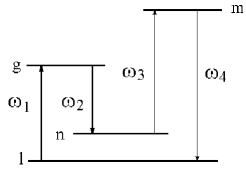
FIG. 5: Coupled transitions.

This section is devoted to investigation of mutual influence of quantum interference, relaxation, incoherent pump of levels, Doppler broadening, effects of strong fields on $FWM$ nonlinear polarization, and absorption of coupled radiations in the context of experiments [11]. We shall consider Raman like coupling (FIG.5) and $FWM$ processes of a type $\omega_{4}=\omega_{1}-\omega_{2}+\omega_{3}$ as well as inverse process $\omega_{3}=\omega_{4}-\omega_{1}+\omega_{2}$. That allows to compare influence of the above discussed elementary effects on conversion processes in different conditions. The elementary quantum mechanical processes, determining $FWM$, essentially depend on that whether the atom at an energy level couples with two strong fields or with one strong and one weak field.

In the range of negligibly small change of the strong radiations both due to absorption and conversion and assuming exact phase-matching, quantum efficiency of conversion $E_{3}$ in $E_{4}$ $\eta_{q4}(\omega_{2})=(k_{3}/k_{4})|E_{4}(z)/E_{3}|^{2}$ can be presented in the form:

$$\eta_{q4}=k_{3}k_{4}{\mid 2\pi N\chi^{(3)}_{4}E_{1}E_{2}^{*}/(\Delta\alpha/2)\mid^{2}}exp\{-\alpha_{4}z\}(exp\{-(\Delta\alpha/2)z\}-1)^{2},$$ (17)

where $N$ – atomic number density, $\chi^{(3)}_{4}$ – nonlinear susceptibility, $\Delta\alpha=\alpha_{1}+\alpha_{2}+\alpha_{3}-\alpha_{4}\approx\alpha_{3}-\alpha_{4}$, $\alpha_{j}$ – absorption index for corresponding radiation. Quantum efficiency for conversion of $E_{4}$ in $E_{3}$ is written in symmetrical form by substitution of $\chi_{4}^{(3)},\alpha_{4}$ for $\chi_{3}^{(3)},\alpha_{3}$. For small length $z<<min\{(\alpha_{4,3})^{-1},(\Delta\alpha/2)^{-1}\}$ spectral features of conversion is determined only by nonlinear susceptibility and by intensities of the strong fields.

$$\eta_{q4,3}=k_{3}k_{4}\mid 2\pi N\chi^{(3)}_{4,3}E_{1}E_{2}\mid^{2}z^{2}$$ (18)

A $FWM$ in two strong and one weak fields at the conditions of maximum coherence and coherent population trapping

In this section expressions for nonlinear polarization at frequencies $\omega_{3}$ and $\omega_{4}$ will be presented for cases, when the fields $E_{1}$ and $E_{2}$ are strong. Their frequencies $\omega_{1}$ and $\omega_{2}$ are close accordingly to the transition frequencies $\omega_{lg}$ and $\omega_{ng}$. Radiations $E_{3}$ and $E_{4}$ with frequencies $\omega_{3}$ and $\omega_{4}$, close to the transition frequencies $\omega_{nm}$ and $\omega_{lm}$ - are supposed nonperturbatively weak. $NIE$ in two strong fields may give rise to such population transfer between levels $l$ and $n$ that population of the intermediate level $g$ change negligibly. Such behavior is similar to $CPT$ (for review see [20]). In more general sense a term $CPT$ is often applied to the processes whereas contribution of $NIE$ in population transfer is crucial. Such type of coupling will be considered in this section.

Nonlinear $FWM$ susceptibilities $\tilde{\chi}^{(3)}_{3,4}$ are determined by the equations:

$$P^{NL}(\omega_{3})=N\tilde{\chi}^{(3)}_{3}E_{1}^{*}E_{2}E_{4},\quad P^{NL}(\omega_{4})=N\tilde{\chi}^{(3)}_{4}E_{1}E_{2}^{*}E_{3}.$$ (19)

Expressions for $\tilde{\chi}_{3,4}$ as well as for absorption (refractive) susceptibilities $\chi_{i}$, derived with density matrix in similar way as that in Section II, are given by [21]:

$$\tilde{\chi}_{3}=\dfrac{-iK}{d_{3}(1+q_{2})}\left[\dfrac{R_{1}^{*}}{P_{1}^{*}}\left(\dfrac{1}{P_{41}}+\dfrac{1}{P_{12}^{*}}\right)+\dfrac{R_{2}}{P_{2}P_{12}^{*}}+\dfrac{R_{4}}{P_{4}P_{41}}\right],$$

$$\tilde{\chi}_{4}=\dfrac{-iK}{d_{4}(1+q_{1})}\left[\dfrac{R_{1}}{P_{1}P_{12}}+\dfrac{R_{2}^{*}}{P_{2}^{*}}\left(\dfrac{1}{P_{32}}+\dfrac{1}{P_{12}}\right)+\dfrac{R_{3}}{P_{3}P_{32}}\right],$$ (20)

$$\chi_{i}/\chi_{i}^{0}=\Gamma_{i}{R_{i}}/{P_{i}}{\Delta n_{i}},R_{1}=[{(1+g_{2}^{*})\Delta r_{1}-u_{1}^{*}\Delta r_{2}}]/({1+g_{2}^{*}+u_{2}}),R_{2}=[{(1+u_{2}^{*})\Delta r_{2}-g_{3}\Delta r_{1}}]/({1+g_{2}+u_{2}^{*}}),$$

$$R_{3}=\dfrac{\Delta r_{3}(1+q_{1})-u_{3}R_{2}^{*}(1-q_{3})+q_{1}u_{2}R_{1}}{1+q_{1}+u_{4}},\quad R_{4}=\dfrac{\Delta r_{4}(1+q_{2})-g_{1}R_{1}^{*}(1-q_{4})+q_{2}g_{2}R_{2}}{1+q_{2}+g_{4}}.$$

$$g_{1}=\dfrac{|G_{1}|^{2}}{P_{41}P_{1}^{*}},g_{2}=\dfrac{|G_{1}|^{2}}{P_{12}^{*}P_{2}},g_{3}=\dfrac{|G_{1}|^{2}}{P_{12}^{*}P_{1}^{*}},g_{4}=\dfrac{|G_{1}|^{2}}{P_{41}P_{4}},u_{1}=\dfrac{|G_{2}|^{2}}{P_{12}^{*}P_{2}},u_{2}=\dfrac{|G_{2}|^{2}}{P_{12}P_{1}},u_{3}=\dfrac{|G_{2}|^{2}}{P_{32}P_{2}^{*}},u_{4}=\dfrac{|G_{2}|^{2}}{P_{32}P_{3}},$$

$$q_{1}=\dfrac{|G_{1}|^{2}}{P_{32}d_{4}},q_{2}=\dfrac{|G_{2}|^{2}}{P_{41}d_{3}},q_{3}=\dfrac{|G_{1}|^{2}}{P_{12}d_{4}},q_{4}=\dfrac{|G_{2}|^{2}}{P_{12}^{*}d_{3}},\Delta r_{1}=\dfrac{\Delta n_{1}X_{2}-\Delta n_{2}X_{3}}{X_{1}X_{2}-X_{3}X_{4}},\Delta r_{2}=\dfrac{\Delta n_{2}X_{1}-\Delta n_{1}X_{4}}{X_{1}X_{2}-X_{3}X_{4}},$$

$$d_{3}=\Gamma_{3}+i(\Omega_{4}-\Omega_{1}+\Omega_{2}),d_{4}=\Gamma_{4}+i(\Omega_{1}-\Omega_{2}+\Omega_{3}),$$

$$r_{j}=n_{j}+\Delta r_{2}(b_{1}^{j}\hbox{\ae}_{1}F_{2}+b_{2}^{j}\hbox{\ae}_{2}F_{3})-\Delta r_{1}(b_{1}^{j}\hbox{\ae}_{1}F_{1}+b_{2}^{j}\hbox{\ae}_{2}F_{4}),$$

$$X_{1}=1+a_{1}\hbox{\ae}_{1}F_{1}-a_{2}\hbox{\ae}_{2}F_{4},\quad X_{2}=1+a_{3}\hbox{\ae}_{2}F_{3}-a_{4}\hbox{\ae}_{1}F_{2},$$

$$X_{3}=a_{2}\hbox{\ae}_{2}F_{3}-a_{1}\hbox{\ae}_{1}F_{2},\quad X_{4}=a_{4}\hbox{\ae}_{1}F_{1}-a_{3}\hbox{\ae}_{2}F_{4}.$$ (21)

$$F_{1}=Re\{\dfrac{\Gamma_{1}}{P_{1}}\dfrac{1+g_{2}^{*}}{1+g_{2}^{*}+u_{2}}\},F_{2}=Re\{\dfrac{\Gamma_{1}}{P_{1}}\dfrac{u_{1}^{*}}{1+g_{2}^{*}+u_{2}}\},F_{3}=Re\{\dfrac{\Gamma_{2}}{P_{2}^{*}}\dfrac{1+u_{2}}{1+g_{2}^{*}+u_{2}}\},F_{4}=Re\{\dfrac{\Gamma_{2}}{P_{2}^{*}}\dfrac{g_{3}^{*}}{1+g_{2}^{*}+u_{2}}\}.$$

Here and further $\Delta r_{1}=r_{l}-r_{g},\Delta r_{2}=r_{n}-r_{g},\Delta r_{3}=r_{n}-r_{m},\Delta r_{4}=r_{l}-r_{m},\Delta n_{4}=n_{l}-n_{m}$, etc., $r_{j}$ and $n_{j}$ are population of levels accordingly power dependent and in absence of the fields; $\hbox{\ae}_{1}$, $\hbox{\ae}_{2}$ – saturation parameters; $a_{k}$, $b_{k}^{j}$ - coefficients, determined by relaxation properties of the transitions, which are different for open and closed transition configurations and will be defined below; $K$ is constant.
OPEN CONFIGURATIONS
For the open system the parameters in (A)are:

$$\hbox{\ae}_{1}=\dfrac{2|G_{1}|^{2}(\Gamma_{g}+\Gamma_{l}-\gamma_{1})}{\Gamma_{g}\Gamma_{l}\Gamma_{1}},\quad\hbox{\ae}_{2}=\dfrac{2|G_{2}|^{2}(\Gamma_{g}+\Gamma_{n}-\gamma_{2})}{\Gamma_{g}\Gamma_{n}\Gamma_{2}},$$

$$a_{2}=\dfrac{\Gamma_{n}}{\Gamma_{l}}\dfrac{\Gamma_{l}-\gamma_{1}}{\Gamma_{g}+\Gamma_{n}-\gamma_{2}},\quad a_{4}=\dfrac{\Gamma_{l}}{\Gamma_{n}}\dfrac{\Gamma_{n}-\gamma_{2}}{\Gamma_{l}+\Gamma_{g}-\gamma_{1}},\quad a_{1}=a_{3}=1,$$

$$b_{1}^{g}=-\dfrac{\Gamma_{l}}{\Gamma_{l}+\Gamma_{g}-\gamma_{1}},\quad b_{2}^{g}=\dfrac{\Gamma_{n}}{\Gamma_{g}+\Gamma_{n}-\gamma_{2}},\quad b_{1}^{n}=-\dfrac{\gamma_{2}}{\Gamma_{n}}b_{1}^{g},\quad$$

$$b_{2}^{n}=-\dfrac{\Gamma_{g}-\gamma_{2}}{\Gamma_{g}+\Gamma_{n}-\gamma_{2}},\quad b_{1}^{l}=\dfrac{\Gamma_{g}-\gamma_{1}}{\Gamma_{l}+\Gamma_{g}-\gamma_{1}},\quad b_{2}^{l}=\dfrac{\gamma_{1}}{\Gamma_{l}}b_{2}^{g},\quad b_{i}^{m}=0.$$

CLOSED CONFIGURATION
The corresponding parameters in (A) take the values:

$$\hbox{\ae}_{1}={4|G_{1}|^{2}}/{\Gamma_{g}\Gamma_{1}},a_{1}=0.5[1+\Delta n_{1}(1+{\gamma_{2}}/{\Gamma_{n}})],a_{2}=1+\Delta n_{1}-(1+2\Delta n_{1})({\Gamma_{g}-\gamma_{2}})/({\Gamma_{g}+\Gamma_{n}-\gamma_{2}}),$$

$$a_{3}=1+\Delta n_{2}[1-2({\Gamma_{g}-\gamma_{2}})/({\Gamma_{g}+\Gamma_{n}-\gamma_{2}})],a_{4}=0.5[1-({\gamma_{2}}/{\Gamma_{n}})+\Delta n_{2}[1+({\gamma_{2}}/{\Gamma_{n}})],$$

$$b_{1}^{l}/n_{l}=b_{1}^{m}/n_{m}=({\Gamma_{n}+\gamma_{2}})/{2\Gamma_{n}},b_{2}^{l}/n_{l}=b_{2}^{l}/n_{l}=-({\Gamma_{n}-\Gamma_{g}+\gamma_{2}})/({\Gamma_{g}+\Gamma_{n}-\gamma_{2}}),$$

$$b_{1}^{n}=0.5n_{n}-(1-n_{n}){\gamma_{2}}/{2\Gamma_{n}},b_{2}^{n}=(2n_{n}-1)({\Gamma_{g}-\gamma_{2}})/({\Gamma_{g}+\Gamma_{n}-\gamma_{2}})-n_{n},$$

$$b_{1}^{g}=n_{g}({\Gamma_{n}+\gamma_{2}})/{2\Gamma_{n}}-0.5,b_{2}^{g}=1-n_{g}-(1-2n_{g})({\Gamma_{g}-\gamma_{2}})/({\Gamma_{g}+\Gamma_{n}-\gamma_{2}}),$$

$$n_{l}={(1+w_{m}/\Gamma_{m}+w_{g}/\Gamma_{g}+w^{\prime}_{n}/\Gamma_{n})}^{-1},n_{m}=w_{m}n_{l}/\Gamma_{m},n_{g}=w_{g}n_{l}/\Gamma_{g},$$

$$n_{n}=w_{n}^{\prime}n_{l}/\Gamma_{n},w_{n}^{\prime}=w_{n}+w_{g}\gamma_{gn}/\Gamma_{g}+w_{m}\gamma_{mn}/\Gamma_{m}$$

B $FWM$ of two strong and two weak radiations under condition of perturbation of each resonant energy level only by one strong radiation

In [11] the features coming out from increase of intensity of a radiation at frequency $\omega_{3}$ were investigated too. Consider a case, where the fields $E_{1}$ and $E_{3}$ are strong, and $E_{2}$ and $E_{4}$ - weak. With the aid of solution of a set of equations for off- and diagonal elements of density matrix up to the first order of perturbation theory in respect of the weak fields equations for the susceptibilities can be presented as [22]:

$$\tilde{\chi}_{2}=\dfrac{-iK}{d_{2}(1+v_{5}^{*}+g_{5}^{*})}\left[\left(\dfrac{\Delta r_{1}}{P_{1}P_{41}^{*}}+\dfrac{\Delta r_{3}}{P_{3}P_{43}^{*}}\right)+\dfrac{R_{4}^{*}}{P_{4}^{*}}\left(\dfrac{1}{P_{41}^{*}}+\dfrac{1}{P_{43}^{*}}\right)\right],v_{5}=\dfrac{|G_{3}|^{2}}{P_{41}d_{2}^{*}},g_{5}=\dfrac{|G_{1}|^{2}}{P_{43}d_{2}^{*}},v_{1}=\dfrac{|G_{3}|^{2}}{P_{43}P_{3}^{*}},$$

$$\tilde{\chi}_{4}=\dfrac{-iK}{d_{4}(1+v_{7}^{*}+g_{7}^{*})}\left[\left(\dfrac{\Delta r_{1}}{P_{1}P_{12}}+\dfrac{\Delta r_{3}}{P_{3}P_{32}}\right)+\dfrac{R_{2}^{*}}{P_{2}^{*}}\left(\dfrac{1}{P_{12}}+\dfrac{1}{P_{32}}\right)\right],v_{7}=\dfrac{|G_{3}|^{2}}{P_{12}^{*}d_{4}^{*}},g_{7}=\dfrac{|G_{1}|^{2}}{P_{32}^{*}d_{4}^{*}},v_{2}=\dfrac{|G_{3}|^{2}}{P_{32}^{*}P_{2}},$$ (22)

$$R_{2}=\dfrac{\Delta r_{2}(1+g_{7}+v_{7})-v_{3}(1+v_{7}-g_{8})\Delta r_{3}-g_{3}(1+g_{7}-v_{8})\Delta r_{1}}{(1+g_{2}+v_{2})+[g_{7}+g_{2}(g_{7}-v_{8})+v_{7}+v_{2}(v_{7}-g_{8})]},v_{8}=\dfrac{|G_{3}|^{2}}{P_{32}^{*}d_{4}^{*}},g_{8}=\dfrac{|G_{1}|^{2}}{P_{12}^{*}d_{4}^{*}},v_{3}=\dfrac{|G_{3}|^{2}}{P_{32}^{*}P_{3}^{*}},$$

$$R_{4}=\dfrac{\Delta r_{4}(1+v_{5}+g_{5})-g_{1}(1+g_{5}-v_{6})\Delta r_{1}-v_{1}(1+v_{5}-g_{6})\Delta r_{3}}{(1+g_{4}+v_{4})+[v_{5}+v_{4}(v_{5}-g_{6})+g_{5}+g_{4}(g_{5}-v_{6})]},v_{6}=\dfrac{|G_{3}|^{2}}{P_{43}d_{2}^{*}},g_{6}=\dfrac{|G_{1}|^{2}}{P_{41}d_{2}^{*}},v_{4}=\dfrac{|G_{3}|^{2}}{P_{43}P_{4}},$$

$$d_{2}=\Gamma_{ng}+i(\Omega_{1}+\Omega_{3}-\Omega_{4}),\chi_{i}/\chi_{i}^{0}=\Gamma_{i}{\Delta r_{i}}/{P_{i}}{\Delta n_{i}},(i=1,3),\chi_{i}/\chi_{i}^{0}=\Gamma_{i}{R_{i}}/{P_{i}}{\Delta n_{i}},(i=2,4).$$ (23)

The rest notations are the same as in Subsection III.A. Expressions for the populations are:
OPEN CONFIGURATION

$$\Delta r_{1}=[{(1+\hbox{\ae}_{3})\Delta n_{1}+b_{1}\hbox{\ae}_{3}\Delta n_{3}}]/[{(1+\hbox{\ae}_{1})(1+\hbox{\ae}_{3})-a_{1}\hbox{\ae}_{1}b_{1}\hbox{\ae}_{3}}],$$

$$\Delta r_{3}=[{(1+\hbox{\ae}_{1})\Delta n_{3}+a_{1}\hbox{\ae}_{1}\Delta n_{1}}]/[{(1+\hbox{\ae}_{1})(1+\hbox{\ae}_{3})-a_{1}\hbox{\ae}_{1}b_{1}\hbox{\ae}_{3}}],$$

$$\Delta r_{2}=\Delta n_{2}-b_{2}\hbox{\ae}_{3}\Delta r_{3}-a_{2}\hbox{\ae}_{1}\Delta r_{1},\ \Delta r_{4}=\Delta n_{4}-a_{3}\hbox{\ae}_{1}\Delta r_{1}-b_{3}\hbox{\ae}_{3}\Delta r_{3},$$

$$r_{m}=n_{m}+(1-b_{2})\hbox{\ae}_{3}\Delta r_{3},r_{g}=n_{g}+(1-a_{3})\hbox{\ae}_{1}\Delta r_{1},$$

$$r_{n}=n_{n}-b_{2}\hbox{\ae}_{3}\Delta r_{3}+a_{1}\hbox{\ae}_{1}\Delta r_{1},r_{l}=n_{l}-b_{1}\hbox{\ae}_{3}\Delta r_{3}+a_{3}\hbox{\ae}_{1}\Delta r_{1},$$

$$\hbox{\ae}_{1}=\hbox{\ae}_{1}^{0}\dfrac{\Gamma_{lg}^{2}}{|P_{1}|^{2}},\ \hbox{\ae}_{1}^{0}=\dfrac{2(\Gamma_{l}+\Gamma_{g}-\gamma_{gl})}{\Gamma_{l}\Gamma_{g}\Gamma_{lg}}|G_{1}|^{2},\ \hbox{\ae}_{3}=\hbox{\ae}_{3}^{0}\dfrac{\Gamma_{mn}^{2}}{|P_{3}|^{2}},\ \hbox{\ae}_{3}^{0}=\dfrac{2(\Gamma_{m}+\Gamma_{n}-\gamma_{mn})}{\Gamma_{m}\Gamma_{n}\Gamma_{mn}}|G_{3}|^{2},$$

$$a_{1}=\dfrac{\gamma_{gn}a_{2}}{\Gamma_{n}-\gamma_{gn}}=\dfrac{\gamma_{gn}\Gamma_{l}a_{3}}{\Gamma_{n}(\Gamma_{g}-\gamma_{gl})}=\dfrac{\gamma_{gn}\Gamma_{l}}{\Gamma_{n}(\Gamma_{l}+\Gamma_{g}-\gamma_{gl})},$$

$$b_{1}=\dfrac{\gamma_{ml}\Gamma_{n}b_{2}}{\Gamma_{l}(\Gamma_{m}-\gamma_{mn})}=\dfrac{\gamma_{ml}b_{3}}{\Gamma_{l}(\Gamma_{l}-\gamma_{ml})}=\dfrac{\gamma_{ml}\Gamma_{n}}{\Gamma_{l}(\Gamma_{m}+\Gamma_{n}-\gamma_{mn})}.$$

CLOSED CONFIGURATION
The populations of levels are described by the equations:

$$\Gamma_{m}r_{m}=w_{m}r_{l}-2\hbox{Re}\hskip 0.2pt\left\{iG_{3}^{*}r_{3}\right\},\quad\Gamma_{g}r_{g}=w_{g}r_{l}-2\hbox{Re}\hskip 0.2pt\left\{iG_{1}^{*}r_{1}\right\},$$

$$\Gamma_{n}r_{n}=w_{n}r_{l}+2\hbox{Re}\hskip 0.2pt\left\{iG_{3}^{*}r_{3}\right\}+\gamma_{gn}r_{g}+\gamma_{mn}r_{m},\quad r_{l}=1-r_{m}-r_{g}-r_{n},$$

where $r_{1}=iG_{1}\Delta r_{1}/P_{1}$, $r_{3}=iG_{3}\Delta r_{3}/P_{3}$. The solution is

$$r_{l}=n_{l}(1+\hbox{\ae}_{3})(1+\hbox{\ae}_{1})/\beta,\quad r_{g}=(1+\hbox{\ae}_{3})[n_{l}(1+\hbox{\ae}_{1})-\Delta n_{1}]/\beta,$$

$$r_{n}=\left\{n_{m}(1+\hbox{\ae}_{3})(1+\hbox{\ae}_{1})+[\Delta n_{3}(1+\hbox{\ae}_{1})+\Delta n_{1}\gamma_{2}\hbox{\ae}_{1}/\Gamma_{n}](1+b\hbox{\ae}_{3})\right\}/\beta$$

$$r_{m}=\left\{n_{m}(1+\hbox{\ae}_{3})(1+\hbox{\ae}_{1})+[\Delta n_{3}(1+\hbox{\ae}_{1})+\Delta n_{1}\gamma_{2}\hbox{\ae}_{1}/\Gamma_{n}]b\hbox{\ae}_{3}\right\}/\beta,$$

$$\Delta r_{1}=r_{l}-r_{g}=\Delta n_{1}(1+\hbox{\ae}_{3})/\beta,\qquad\Delta r_{3}=r_{n}-r_{m}=[\Delta n_{3}(1+\hbox{\ae}_{1})+\Delta n_{1}\gamma_{2}\hbox{\ae}_{1}/\Gamma_{n}]/\beta,$$

where $\beta=(1+\hbox{\ae}_{3})[1-\Delta n_{3}+2(n_{l}+n_{m})\hbox{\ae}_{1}]+(1+2b\hbox{\ae}_{3})[\Delta n_{3}(1+\hbox{\ae}_{1})+\Delta n_{1}\gamma_{2}\hbox{\ae}_{1}/\Gamma_{n}]$, $\Delta n_{1}=n_{l}-n_{g}$, $\Delta n_{3}=n_{n}-n_{m}$, $n_{m}=n_{l}w_{m}/\Gamma_{m}$, $n_{g}=n_{l}w_{g}/\Gamma_{g}$, $n_{n}=n_{l}{w_{n}}^{\prime}/\Gamma_{n}$, $n_{l}=(1+w_{m}/\Gamma_{m}+w_{g}/\Gamma_{g}+{w_{n}}^{\prime}/\Gamma_{n})^{-1}$, ${w_{n}}^{\prime}=w_{n}+w_{g}\gamma_{gn}/\Gamma_{n}+w_{m}\gamma_{mn}/\Gamma_{n}$, $b=\Gamma_{n}/(\Gamma_{m}+\Gamma_{n}-\gamma_{3})$, $\hbox{\ae}_{1}=({2|G_{1}|^{2}}/{\Gamma_{1}\Gamma_{g}})({\Gamma_{1}^{2}}/{|P_{1}|^{2}})$, $\hbox{\ae}_{3}=({2|G_{3}|^{2}(\Gamma_{m}+\Gamma_{n}-\gamma_{3})}/{\Gamma_{m}\Gamma_{n}\Gamma_{3}})({\Gamma_{3}^{2}}/{|P_{3}|^{2}})$. The remaining denotations are former.

C Effect of Doppler broadening on resonant $FWM$

Formula for $\tilde{\chi}_{4}^{(3)}$ in lowest order of perturbation theory [18] can be derived from (A), (22) at $G_{i}\rightarrow 0$:

$$\tilde{\chi}_{4}^{(3)}(\omega_{4}=\omega_{1}-\omega_{2}+\omega_{3})=\dfrac{iK}{\Gamma_{ml}+i(\Omega^{{}^{\prime}}_{1}-\Omega^{{}^{\prime}}_{2}+\Omega^{{}^{\prime}}_{3})}\cdot$$

$$\cdot\left\{\dfrac{1}{\Gamma_{gm}+i(\Omega^{{}^{\prime}}_{3}-\Omega^{{}^{\prime}}_{2})}\cdot[\dfrac{n_{g}-n_{n}}{\Gamma_{ng}-i\Omega^{{}^{\prime}}_{2}}+\dfrac{n_{m}-n_{n}}{\Gamma_{mn}+i\Omega^{{}^{\prime}}_{3}}]+\dfrac{1}{\Gamma_{ln}+i(\Omega^{{}^{\prime}}_{1}-\Omega^{{}^{\prime}}_{2})}\cdot[\dfrac{n_{g}-n_{n}}{\Gamma_{ng}-i\Omega^{{}^{\prime}}_{2}}+\dfrac{n_{g}-n_{l}}{\Gamma_{lg}+i\Omega^{{}^{\prime}}_{1}}]\right\},$$ (24)

where $\Omega^{{}^{\prime}}_{j}=\Omega_{j}-{\bf k}_{j}{\bf v}$, $n_{i}=N_{i}\cdot exp\{-({\bf v}/\bar{v})^{2}\}/\sqrt{\pi}\bar{v}$. As the function of $v$ all terms in (24), besides those proportional to $n_{g}-n_{n}$, have all poles in one and the same complex half plane. Therefore at $\Gamma_{i}<<k_{i}\bar{v}$ only terms, proportional to $n_{g}-n_{n}$, do not vanish after averaging over Maxwell’s velocity distribution. Velocity averaged susceptibility is:

$$<\tilde{\chi}_{4}^{(3)}(\omega_{4})>_{v}=\dfrac{iK\pi^{1/2}\exp\{-(\Omega_{2}/k_{2}\bar{v})^{2}\}(N_{g}-N_{n})}{k_{2}\bar{v}[\tilde{\Gamma}_{1}+i(\Omega_{1}-k_{1}\Omega_{2}/k_{2})][\tilde{\Gamma}_{3}+i(\Omega_{3}-k_{3}\Omega_{2}/k_{2})]},$$ (25)

$$\tilde{\Gamma}_{1}=\Gamma_{nl}+({k_{1}/k_{2}}-1)\Gamma_{ng},\quad\tilde{\Gamma}_{3}=\Gamma_{gm}+({k_{3}/k_{2}}-1)\Gamma_{ng}.$$

As it is seen from (25), for the process $\omega_{4}=\omega_{1}-\omega_{2}+\omega_{3}$ interference of contributions of atoms at different velocities to the velocity averaged nonperturbed $FWM$ nonlinear susceptibility $<\tilde{\chi}_{4}>_{v}$ leads to the fact, that in the lowest order on the small parameter $\Gamma_{2}/k_{2}\bar{v}$, it is proportional to the velocity integrated difference between populations of the excited states $N_{g}-N_{n}$. In the similar way, with aid of (22) one can find, that on the contrary, $<\tilde{\chi}_{2}>_{v}$ for the process $\omega_{2}=\omega_{1}-\omega_{4}+\omega_{3}$ in the same approximation is determined by the population difference on transitions from the lowest level. For the resonant sum frequency $FWM$ $\omega_{4}=\omega_{1}+\omega_{2}+\omega_{3}$ in the cascade configuration of levels velocity averaged susceptibility occurs proportional to higher order of the small parameter $\Gamma/k\bar{v}$ compared to Raman-type difference-frequency coupling [2]. These features demonstrate great difference between resonant $FWM$ processes in homogeneously and inhomogeneously broadened transitions.

In strong electromagnetic fields above mentioned processes are accompanied by the velocity selective population transfer and by some other intensity dependent effects. In [11] experiments on resonant $cw$ $FWM$ at Raman-like electronic molecular transitions of $Na_{2}$ have been carried out. Frequency tunable radiation at $\omega_{2}$ was generated at the same transition of $Na_{2}$ either in external dimer Raman laser or $FWM$ was performed inside the Raman laser cavity. Frequency $\omega_{2}$ was tuned by tuning $\omega_{1}$. Radiation at $\omega_{3}$ was provided from $cw$ dye laser. High conversion efficiency have been attained in single frequency nearly power saturation regime. Observed $FWM$ frequency tuning characteristics occured in disagreement with the predictions of lowest order perturbative theory. From that the authors derived the questions to be answered with the aid of an advanced nonperturbative theory. We shall use above presented expressions for the numerical analysis of the models with the parameters, close to that in the experiments, in order to explain main observed features.

The electronic - vibration-rotation transitions between $X$, $A$ and $B$ electronic levels of the dimer were used in the experiments, the lowest electronic level being ground one. Two $FWM$ processes were investigated: when frequency $\omega_{3}$ less than $\omega_{2}$ and, therefore frequency of a generated radiation $\omega_{4}$ was less than $\omega_{1}$ (down conversion) and opposite upconversion process. As it was discussed above, different appearances of interference processes at Doppler broadened transitions can be expected in those cases. Main observed experimental dependencies, which did not find explanations, can be summarized as follows.

According to (25), at $\Omega_{1}-k_{1}\Omega_{2}/k_{2}=0$, in the lowest order of perturbation theory the maximum output of $FWM$ at $\omega_{4}$ as a function of $\omega_{3}$ corresponds to $\Omega_{3}=k_{3}\Omega_{2}/k_{2}=0$. Lineshape of the resonance is Lorentzian with the linewidth of the order of characteristic homogeneous widths of optical transitions. However, in the down conversion experiments the wide resonance of the order of Doppler width of transition $ml$ with the center being locked at $\omega_{3}\approx\omega_{mg}$ was observed. It’s position practically did not vary at tuning $\omega_{2}$ within Doppler resonance of the transition $gn$ (at the expense of tuning of $\omega_{1}$, so that $\Omega_{2}=k_{2}\Omega_{1}/k_{1}$). In the upconversion experiments the resonance was tunable by tuning frequency $\omega_{2}$, but with the slope less than $d\Omega_{3}/d\Omega_{2}=k_{3}/k_{2}$. Width of the resonance also was commensurable with the Doppler width of the transition $ml$.

For numerical analysis we have used a model with the transitions parameters, close to those from the experiment.
1. Down conversion: $\lambda_{ml}$ = 598 nm, $\lambda_{gl}$ = 488 nm, $\lambda_{mn}$ = 655 nm, $\lambda_{gn}$ = 525 nm; $k_{1}\bar{v}=6.94$, $k_{2}\bar{v}=6.45$, $k_{3}\bar{v}=5.17$, $k_{4}u=5.66$, (in terms of $10^{9}$ $c^{-1}$); $\Gamma_{m}=200$, $\Gamma_{n}=30$, $\Gamma_{g}=260$, $\gamma_{mn}=2$, $\gamma_{ml}=4$, $\gamma_{gn}=20$, $\gamma_{gl}=10$, $\Gamma_{ln}=40$, $\Gamma_{nm}=110$, $\Gamma_{lm}=110$, $\Gamma_{gm}=130$, $\Gamma_{ng}=140$, $\Gamma_{lg}=140$, (in terms of $10^{6}$ $c^{-1}$) $N_{l}/N_{n}=30/2$.

2. Up-conversion: $\lambda_{ml}$ = 473 nm, $\lambda_{gl}$ = 661 nm, $\lambda_{mn}$ = 514 nm, $\lambda_{gn}$ = 746 nm; $k_{1}\bar{v}=5.12$, $k_{2}\bar{v}=4.54$, $k_{3}\bar{v}=6.59$, $k_{4}\bar{v}=7.16$, (in terms of $10^{9}$ $c^{-1}$); $\Gamma_{m}=200$, $\Gamma_{n}=30$, $\Gamma_{g}=260$, $\gamma_{mn}=2$, $\gamma_{ml}=4$, $\gamma_{gn}=20$, $\gamma_{gl}=10$, $\Gamma_{ln}=40$, $\Gamma_{nm}=110$, $\Gamma_{lm}=110$, $\Gamma_{gm}=130$, $\Gamma_{ng}=140$, $\Gamma_{lg}=140$, (in terms of $10^{6}$ $c^{-1}$), $N_{l}/N_{n}=110/3.2$, population of two upper levels being negligibly small.

First, with an aid of these models we shall illustrate a role of an interference at velocity averaging of nonlinear susceptibilities in weak fields. For down conversion in exact one- and multiphoton resonances and homogeneously broadened transitions computing gives the ratio of squared modulus of nonlinear susceptibilities $|\chi_{3}^{(3)}/\chi_{4}^{(3)}|^{2}$ = 2.5. For averaged values it yields $|<\chi_{3}^{(3)}>_{v}/<\chi_{4}^{(3)}>_{v}|^{2}$ = $2.31\cdot 10^{2}$. If to change the population ratio for the inverse magnitude ($N_{n}/N_{l}=30/2$), we obtain: $|\chi_{3}^{(3)}/\chi_{4}^{(3)}|^{2}$ = 0.4. The difference between averaged values sharply decreases. Their ratio in this case yields: $|<\chi_{3}^{(3)}>_{v}/<\chi_{4}^{(3)}>_{v}|^{2}$ = 0.13.

For up-conversion similar computations give: $|\chi_{3}^{(3)}/\chi_{4}^{(3)}|^{2}$ = 2.7, $|<\chi_{3}^{(3)}>_{v}/<\chi_{4}^{(3)}>_{v}|^{2}$ = $1.45\cdot 10^{3}$. At the inverse population ratio ($N_{n}/N_{l}=110/3.2$) we obtain: $|\chi_{3}^{(3)}/\chi_{4}^{(3)}|^{2}$ = 0.37. The difference between averaged values sharply decreases. Their ratio in this case is: $|<\chi_{3}^{(3)}>_{v}/<\chi_{4}^{(3)}>_{v}|^{2}$ = 0.24.

Thus, effect of inhomogeneous broadening of the resonant transitions on $FWM$ processes may be very strongly dependent on a specific process, as well as on distribution of the populations over levels and velocities. Therefore one can expect that velocity selective population transfer and other effects of strong fields may change conclusions of the lowest order perturbative theory.

For small number density and medium length $FWM$ conversion efficiency of weak radiation is proportional to a product of intensities of the strong radiations and squared modulus of velocity averaged nonlinear susceptibility (equation (18)). The later is intensity dependent too. Further we shall numerically analyze effects of the strong fields on conversion efficiency with an aid of the expressions of the subsections III.A and III.B. Intensities of the radiations will be characterized by the parameters $S_{1}=|G_{1}|^{2}/\Gamma_{gl}\Gamma_{nl}$ and $S_{2}=|G_{2}|^{2}/\Gamma_{gn}\Gamma_{nl}$, which are chosen in near saturation range like in the experiments.

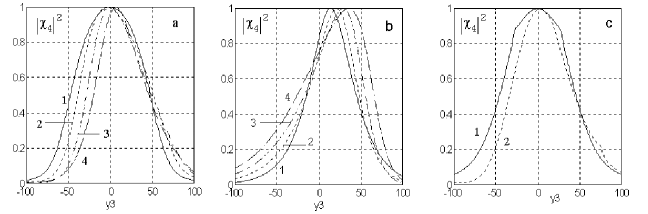
FIG. 6: Squared modulus of scaled velocity averaged nonlinear susceptibility $|<\chi^{(3)}_{4}>_{v}/<\chi^{(3)}_{40}>_{v}|^{2}$ vs scaled detuning $y_{3}=\Omega_{3}/\Gamma_{nm}$ at various detunings $\Omega_{1}$ ($\Omega_{2}=k_{2}/k_{1}\Omega_{1}$. a and b: upconversion, $S_{1}=150$, $S_{2}=350$); a: 1 – $\Omega_{1}=0$, 2 – $\Omega_{1}=10\Gamma_{lg}$, 3 – $\Omega_{1}=20\Gamma_{lg}$, 4 – $\Omega_{1}=30\Gamma_{lg}$; b: 1 -$\Omega_{1}=40\Gamma_{lg}$, 2 – $\Omega_{1}=50\Gamma_{lg}$, 3 – $\Omega_{1}=60\Gamma_{lg}$, 4 – $\Omega_{1}=70\Gamma_{lg}$. c: downconversion; $S_{1}=1000$, $S_{2}=2000$; 1 - $\Omega_{1}=0$, 2 - $\Omega_{1}=50\Gamma_{lg}$.

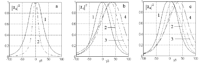
FIG. 7: Squared modulus of scaled velocity averaged nonlinear susceptibility $|<\chi^{(3)}_{4}>_{v}/<\chi^{(3)}_{40}>_{v}|^{2}$ vs scaled detuning $y_{3}=\Omega_{3}/\Gamma_{nm}$ at various detunings $\Omega_{1}$ ($\Omega_{2}=k_{2}/k_{1}\Omega_{1}$) (upconversion, each level is coupled to only one strong field). a: $\Omega_{1}=0$, $S_{1}=1000$; 1 – $S_{3}=1000$, 2 – $S_{3}=1600$. b: $S_{1}=2000$, $S_{3}=2100;$ 1 – $y_{1}=0$, 2 – $y_{1}=20$, 3 – $y_{1}=40$, 4 – $y_{1}=60$. c: same as in b, but $S_{1}=4000$, $S_{3}=4200$.

Figures 6 show, that for the chosen parameters due to power broadening the resonance is much broader than homogeneous transition width and is commensurable with Doppler linewidth, which is of the order 60 in the used scale. For the parameters, corresponding to the up-conversion experiments (FIG. 6 a,b) in the range of small detunings $\Omega_{1}$ ($\Omega_{2}=(k_{2}/k_{1})\Omega_{1}$) (FIG. 6 a) the peak of the tuning curve is displaced very insignificantly (and even in the opposite side, depending on the value of $\Omega_{1}$). At further increase of $\Omega_{1}$ (FIG. 6 b) the maximum shifts with the increase of $\Omega_{1}$, so that the slope $\Omega_{3}/\Omega_{1}$ is variable. A maximum of the slope corresponds to the detunings $\Omega_{1}$ of about a half of Doppler width of the transition $gl$. Thus for the considered intensities the value of the slope reaches $\approx 0.8$, that makes $\approx 0.5(k_{3}/k_{1})$.

FIG. 6 c is computed and drown for the parameters, corresponding to down conversion experiments. For the considered intensities the peak occurs locked to the center of transition $ml$ practically in all an interval of $\Omega_{1}$ within the Doppler width of transition $gl$.

When the weak field detunings are fixed and driving fields frequencies $\omega_{1}$ and $\omega_{2}$ ($\Omega_{2}=(k_{2}/k_{1})\Omega_{1}$) are tuned to the maximum, computer analysis of the slope $d\Omega_{1}/d\Omega_{3}$ in the range of $S_{1}=65,S_{2}=2.33\cdot S_{1}$ shows behavior similar to that observed in experiments [11] ($d\Omega_{1}/d\Omega_{3}\approx k_{1}/2k_{3}$). (Ratio $S_{1}/S_{2}=2.33$ is chosen according to the ratio of prodacts of experimental field intensities and Franck-Kondon factors.)

In the experiments [11] the features, following increase of intensity of $E_{3}$, were observed too. In order to consider effects of this field and to understand whether $CPT$ play a decisive role in observed dependencies we have carried out numerical analysis of the up-conversion model with aid of formulas from the Subsection III.B (FIG. 7).

FIG. 7 a shows that at certain ratio of intensities even power narrowing of Doppler broadened $FWM$ resonance may happen. FIG. 7 b displays approximately constant slope $d\Omega_{3}/d\Omega_{1}$ ($\Omega_{3}$ corresponds to the maximum output), which is about 0.75, in a quite wide interval of $\Omega_{1}$. Only for $\Omega_{1}$, larger than Doppler width, the slope starts decreasing. At larger intensities the slope varies more considerable, when $\Omega_{1}$ is tuned within the Doppler line. So for FIG. 7 c the slope makes up 0.1 in the vicinity of $y_{1}=20$; 0.8 - in the range of $y_{1}=40$ and 0.6 - at $y_{1}=60$.

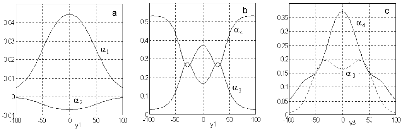
FIG. 8: Velocity-averaged absorption/gain indices scaled to the nonperturbed absorption index at $\omega=\omega_{gl}$ $<\alpha_{i}>_{v}/<\alpha_{1}^{0}>_{v}$ at $S_{1}=150$, $S_{2}=350$ (upconversion). a – absorption of strong radiations vs $\omega_{1}$ ($\Omega_{2}=k_{2}/k_{1}\Omega_{1}$); change in absorption of converting and generated radiations as tuning $\omega_{1}$ ($\Omega_{3}=0$) (b ) and $\omega_{3}$ ($\Omega_{1}=0$) (c ).

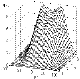
FIG. 9: Effect absorption on $FWM$.

In an absorbing medium spectral properties of absorption indices may bring important effect on $FWM$. FIG. 8 a-c display corresponding lineshapes. FIG. 9 is computed with aid of formula (17) and shows that additional broadening of the tuning curve of $FWM$ output may arise from the propagation effect in an absorbing medium ($Z=\alpha_{10}z$, $\Omega_{1}=0,S_{1}=150,S_{2}=350$ (upconversion)).

In conclusion, the theory of nonlinear interference processes at Doppler broadened quantum transitions in two strong resonant optical fields is developed. The derived formulas allow one account for such contributing processes relevant to experiments as various relaxation channels, incoherent excitation by an external source, population transfer and other coherent and incoherent effects accompanying coupling with strong optical fields in various open and closed configuration of transitions. Explicit formulae accounting for the effects of the strong fields are derived. Such appearance of quantum interference as amplification (and lasing) without inversion of power saturated populations and specific effects in resonant four wave mixing in gases are analyzed with the aid of numerical models. Parameters of the model are close to those of some recently carried out experiments. Crucial effect of Doppler-broadening on the contributions of the populations of different levels to four-wave mixing, which determine selection of optimal energy-level configuration and conditions for the experiments, is shown. Unexpected dependencies, observed in the experiments are explained.

ACKNOWLEDGMENTS

The author would like to thank S. A. Myslivets and V. M. Kuchin for assistance in calculations, A. A. Apolonskii, S. A. Babin, U. Hinze and B. Wellegehausen for useful discussion of their experiments prior publication. This work was supported by the Russian Foundation for Basic Research and by the Deutsche Forschungsgemeinschaft through collaborative Grant 96-02-00016 G. The author wishes to express his sincere thanks to L. J. F. Hermans from Hygens Laboratorium and the Netherlands Science Foundation (NWO) for support of this work.

References

• [1] S. G. Rautian, G. I. Smirnov and A. M. Shalagin, Nonlinear resonances in spectra of atoms and molecules (in Russ.), Nauka, Novosibirsk, 1979; S. G. Rautian and A. M. Shalagin, Kinetic Problems of Nonlinear Spectroscopy, North Holland, Amsterdam, 1991.
• [2] A. K. Popov, Introduction in Nonlinear Spectroscopy (in Russ.), Nauka, Novosibirsk, 1983.
• [3] G. E. Notkin, S. G. Rautian, A. A. Feoktistov, Zh. Eksp. Teor. Fiz., Vol. 52, No 6, 1673, 1967.
• [4] T. Ya. Popova, A. K. Popov, S. G. Rautian, R. I. Sokolovskii, JETP, Vol. 30, 466, 1970 (Zh. Eksp. Teor. Fiz., Vol. 57, 850, 1969), quant-ph/0005094.
• [5] S. G. Rautian and I. I. Sobelman, Zh. Eksp. Teor. Fiz., Vol.41, 456, 1961.
• [6] T. Ya. Popova and A. K. Popov, Zh. Eksp. Teor. Fiz., Vo. 52, 456, 1967; T. Ya. Popova and A. K. Popov, Journ. Appl. Spectr. (Sov.), 12, 734, 1970, Consultants Bureau, Plenum, N.Y., quant-ph/0005047; T. Ya. Popova and A. K. Popov, Sov. Phys. Journ., 13, 1435, 1970, Consultants Bureau, Plenum, N.Y., quant-ph/0005049.
• [7] I. M. Beterov, V. P. Chebotaev, Pis’ma Zh. Eksp. Teor. Fiz., Vol. 9, 216, 1969; I. M. Beterov, Cand. Diss, 1970; Th. Hansch and P. Toschek, Z.Β Physik, Bd. 236. 213 (1970); V. S. Letokhov and V. P. Chebotaev, Nonlinear Laser Spectroscopy , Springer Verlag, 1997; E. Y. Wu, et al., Phys. Rev. Lett., Vol. 38, 1077, 1977; I. S. Zelikovich, S. A. Pulkin, L. S. Gaida, V. N. Komar, Zh. Eksp. Teor. Fiz., Vol. 94, 76, 1988.
• [8] A. K. Popov, Bul. Russ. Acad. Sci., Physics, Vol. 60 (6), 927, 1996 (Allerton Press, N.Y.),
quant-ph/0005108; Proc. SPIE, Vol. 2798, 231, 1996.
• [9] A. K. Popov and S. G. Rautian, Proc. SPIE, Vol. 2798, 49, 1996, quant-ph/0005114.
• [10] Papers from: ”Atomic Coherence and Interference” (Crested Butte Workshop, 1993). Quantum Optics, 1994. 6, N4; ”Coherent phenomena and amplification without Inversion”. (15th Intern. Conf. on Coher. and Nonlin. Opt.), A. V. Andreev, O. Kcharovskaya, P. Mandel, Editors, Proc. SPIE, Vol. 2798,(1996) and ref. therein.
• [11] S. Babin, U. Hinze, E. Tiemann, B. Wellegehausen, Optics Letts, Vol. 21, 1186, 1996; A. Apolonskii, S. Baluschev, U. Hinze, E. Tiemann, B. Wellegehausen, Appl. Phys. Vol. B64, 435, 1997.
• [12] A. K. Popov, V. M. Kuchin and S. A. Myslivets, JETP, Vol. 86, 244 (1998).
• [13] Im Tkhekde, O. P. Podavalova, A. K. Popov, G. Kh. Tartakovsky, Pis’ma Zh. Eksp. Teor. Fiz. (JETP Lett.), Vol. 24, 8 ,1976; Opt. Commun., Vol. 18, 499, 1976; Im Thek-de, O. P. Podavalova, A. K. Popov and V. P. Ranshikov, Opt. Commun., Vol. 30, 196, 1979; Im Tkhekde, O. P. Podavalova, A. K. Popov, Opt. Spektr., Vol. 67, 263, 1989.
• [14] V. M. Klementjev, Yu. A. Matjugin and V. P. Chebotaev, Pis’ma Zh. Eksp. Teor. Fiz., Vol. 24, 8 , 1976.
• [15] L. T. Bolotskikh, A. L. Vysotin, Im Thek-de, O. P. Podavalova and A. K. Popov, Appl.Phys., Vol. B35, 249, 1984; V. G. Arkhipkin, A. L. Vysotin, Im Thek-de, O. P. Podavalova and A. K. Popov, Kvant. Elektron.,Vol. 13, 1352, 1986.
• [16] V. G. Arkhipkin and A. K. Popov, Nonlinear Conversion of Light in Gases (in Russ.), Novosibirsk, Nauka, 1987; V. G. Arkhipkin and A. K. Popov, Sov. Phys. Usp., Vol. 30, No 11, 952, 1987 and ref. therein.
• [17] D. A. Coppeta et al., Phys. Rev. Vol. A53, 925, 1996.
• [18] A. B. Budnitskii and A. K. Popov,Opt. Spektr., Vol. 29, 1032, 1970.
• [19] A. K. Popov and B. Wellegehausen, Laser Physics, Vol. 6, 364, 1996.
• [20] B. D. Agap’ev, M. B. Gornyi, B. G. Matisov, Yu. V. Rozhdestvenskii Yu.V. Uspekhi Fis. Nauk. (Sov. Phys. Uspekhi), Vol. 163, 1, 1993.
• [21] A. K. Popov and S. A. Myslivets, (to be published).
• [22] A. K. Popov and S. A. Myslivets, Quantum Electron., Vol. 27 (11), 1004 (1997); Vol. 28 (2), 185 (1998).