Laser Induced Condensation of Bosonic Gases in Traps

Abstract

We consider collective laser cooling of atomic gas in the Festina lente regime, when the heating effects associated with photon reabsorptions are suppressed. We demonstrate that an appropriate sequence of laser pulses allows to condense a gas of trapped bosonic atoms into the ground level of the trap in the presence of collisions. Such condensation is robust and can be achieved in experimentally feasible traps. We extend significantly the validity of our previous numerical studies, and present new analytic results concerning condensation in the limit of rapid thermalization. We discuss in detail necessary conditions to realize all optical condensate in weak condensation regime and beyond.

32.80Pj, 42.50Vk

I Introduction

Laser cooling has led to spectacular results in recent years [1]. So far, however, it has not allowed to reach temperatures for which quantum statistics become important. In particular, evaporative cooling is used to obtain Bose-Einstein condensation of trapped gases [2]. Nevertheless, several groups are pursuing the challenging goal of condensation via all–optical means [3, 4, 5, 6]. The interest in laser–induced condensation stems from the fact that, (a) a laser–cooled system is open and is not necessarilly in thermal equilibrium, i.e. its physics is in principle much richer than that of evaporatively–cooled gases; (b) laser cooling is perhaps the only method which may condense all atoms into the ground state, i.e. reach an effective zero temperature.

In traps of size larger than the inverse wavevector, $k_{L}^{-1}$, the temperatures required for condensation are typically below the photon recoil energy, $E_{R}=\hbar\omega_{R}=\hbar^{2}k_{L}^{2}/2m$, where $m$ is the atomic mass. There exist several laser cooling schemes to reach such temperatures citeVSCPT,Raman. They exploit single atom “dark states”, i.e. states which cannot be excited by the laser, but can be populated via spontaneous emission. The main difficulty in applying dark state cooling for dense gases is caused by light reabsorption. Indeed, these states are not dark with respect to the photons spontaneously emitted by other atoms. Thus, at sufficiently high densities, dark state cooling may cease to work, since multiple reabsorptions can increase the system energy by several recoil energies per atom [9, 10, 11, 12]. In particular, laser induced condensation is feasible only if the reabsorption probability is smaller than the inverse of the number of energy levels accessible via spontaneous emission processes [10].

Several remedies to the reabsorption problem have been proposed. First, the role of reabsorptions increases with the dimensionality. If the reabsorption cross section for trapped atoms is the same as in free space, i.e. $\simeq 1/k_{L}^{2}$, the reabsorptions should not cause any problem in 1D, have to be carefully considered in 2D, and forbid condensation in 3D. Working with quasi-1D or -2D systems is thus a possible way to reduce the role of reabsorptions [13]. The most promising remedy against this problem employs the dependence of the reabsorption probability for trapped atoms on the fluorescence rate $\gamma$, which can be easily adjusted in dark state cooling [14]. In particular, in the so called Festina lente limit, when $\gamma$ is much smaller than the trap frequency $\omega$ [15], the reabsorption processes in which the atoms change energy and undergo heating are suppressed. This regime can be achieved either in Raman cooling [16] by changing the intensity and/or the detuning of the repumping laser, or in systems which simply posses a narrow natural linewidth.

In a series of papers [17, 18, 19, 20] we have investigated collective cooling schemes in traps of realistic size in the Festina lente limit, and we have shown that laser induced condensation is possible. In this paper we present also such investigation taking into account the effects of atom–atom collisions. This paper is, in a sense, a final paper in a series of papers about the Festina lente regime. In the first two of those papers we have generalized dark state (Raman) cooling method beyond the Lamb-Dicke regime, i.e. beyond the regime when the size of the trap is smaller than the laser wavelength[17, 18]. In particular, in the second of these references we have demonstrated the possibility of cooling to an arbitrary state of the trap. We have then applied those methods to samples of atoms and demonstrated possibility of all optical condensation first for the case of an ideal gas [19], and then taking into account elastic interatomic collisions[20]. In all of the above paper we have limited, however, our investigations to relatively small traps with Lamb-Dicke parameter $\eta$ not greater than 5 in 1D, and not greater than 2 in 3D because of numerical complexity. Also, we have considered so far only the regime of weak condensation, when the energy levels of the trapped gas are not yet modified by the mean field interactions. That implied that we could have considered only moderate numbers of atoms in the trap of the order of few hundred up to one thousand.

In this paper we overcome the above mentioned shortcomings. In particular:

• We extend our numerical studies to traps with $\eta=8$ in 1D and $\eta=4$ in 3D.

• We present analytic description of the dynamics in the weak condensation regime and in the limit of rapid thermalization due to elastic collisions.

• We extend our theory beyond the weak condensation regime to the hydrodynamic regime, and present the analytic description of the dynamics in the limit of rapid thermalization using Bogoliubov-Hartree-Fock theory at finite temperature.

• Finally, we present a detailed discussion of requirements that have to be fulfilled in order to achieve experimentally all optical condensation in the Festina lente regime.

The paper is organized as follows. The sections II–IV deal with the weak condensation regime. In section II, we formulate the Master Equation (ME) that describes the combined effects of dark state (Raman) cooling in the Festina Lente regime, and elastic atom–atom collisions. Cooling is dynamical, and consists of sequences of pairs of laser pulses inducing stimulated and spontaneous Raman transitions between the two electronic levels of trapped atoms, $|g\rangle$ and $|e\rangle$. The stimulated Raman transition induces the energy selective transition $|g\rangle\to|e\rangle$ that depopulates all motional states except the ground state which is dark; the spontaneous Raman transition via a third auxiliary level, similarly as standard spontaneous emission, is non-selective, and repumps the atoms from $|e\rangle$ to $|g\rangle$ populating all accessible motional states. The collisions introduce a thermalization mechanism which redistribute the populations of the trap levels according to a Bose–Einstein distribution (BED). In section III we present our numerical results. We simulate the dynamics generated by the ME in 1D and 3D, and show that laser induced condensation into the ground state of the trap is not only possible with collisions, but it is even more robust when they are present. In Section IV we present analytic results concerning the limit of rapid thermalization, in which the state of the system at each instant can be described by the thermal density matrix of the canonical ensemble. We demonstrate here that laser cooling leads to final temperature of the order of $E_{R}$ or less.

In section V we extend our theory beyond the weak condensation regime. This can be done in the rapid thermalization limit, since in that case one can describe the state of the system at each instant to be thermal and well described by the Bogoliubov–Hartree–Fock theory at finite temperature $T$ [21]. Laser cooling introduces then a slow process of decrease of the effective temperature. We show that cooling down to $T\simeq 0$ is also possible beyond the weak condensation regime. This allows us to present a detailed discussion of the prospects for all optical BEC in Section VI.

II Quantum Master Equation

We consider $N$ bosonic atoms with two levels $|g\rangle$ and $|e\rangle$ in a non-isotropic dipole trap with the frequencies $\omega^{g}_{x,y,z},\omega^{e}_{x,y,z}$ different for the ground and the excited states, and non-commensurable one with another. This assumption simplifies enormously the dynamics of the spontaneous emission processes in the Festina Lente limit. We assume weak absorption pulses, so that no significant excited–state population is present. This allows to adiabatically eliminate the excited–state contribution, and consequently to consider the density matrix $\rho(t)$ describing all atoms in the ground state $|g\rangle$, and diagonal in the Fock representation corresponding to the bare trap levels. The ground state $|g\rangle$ into which the condensation will take place, should be the ground electronic state of the atom, in such a way that the inelastic collisions of two $|g\rangle$ atoms are not possible [22]. The Raman lasers are red–detuned sufficiently far from molecular resonances, such that photoassociation losses can be neglected for the regime of atomic densities considered, $n<10^{15}$atoms/cm³ [23]. For these densities, three–body losses are also negligible. We shall show that in the weak condensation regime, when the mean–field energy $E_{I}<\hbar\omega$, the laser–cooling and collisional effects can be considered separately. In particular, the latter ones can be described by a quantum Boltzmann ME [25, 26]. The extension of our results beyond the weak condensation regime ($E_{I}>\hbar\omega$) is discussed in section V.

In the following we follow the same notation as in Refs. [19, 20]. Let $g_{m}$, $g_{m}^{{\dagger}}$ ($e_{l}$, $e_{l}^{{\dagger}}$) be the annihilation and creation operators of atoms in the ground (excited) state and in the trap level $m$ $(l)$, which fulfill the bosonic commutation relations. Using the standard theory of quantum stochastic processes one can develop the quantum ME which describes the atom dynamics in the Festina Lente regime [19]

$$\dot{\rho}(t)={\cal L}_{0}\rho+{\cal L}_{1}\rho+{\cal L}_{2}\rho,$$ (1)

where

$${\cal L}_{0}\rho = -i\hat{H}_{eff}\rho(t)+i\rho(t)\hat{H}_{eff}^{{\dagger}}+{\cal J}\rho(t),$$ (3)

$${\cal L}_{1}\rho = -i[\hat{H}_{las},\rho(t)],$$ (4)

$${\cal L}_{2}\rho = -i[\hat{H}_{coll},\rho(t)],$$ (5)

with

$$\hat{H}_{eff} = \sum_{m}\hbar\omega_{m}^{g}g_{m}^{{\dagger}}g_{m}+\sum_{l}\hbar(\omega_{l}^{e}-\delta)e_{l}^{{\dagger}}e_{l}$$ (7)

$$- i\hbar\gamma\int d\phi d\theta sin\theta{\cal W}(\theta,\phi)$$ (8)

$$\times \sum_{l,m}|\eta_{lm}(\vec{k})|^{2}e_{l}^{{\dagger}}g_{m}g_{m}^{{\dagger}}e_{l},$$ (9)

$$\hat{H}_{las} = \frac{\hbar\Omega}{2}\sum_{l,m}\eta_{lm}(k_{L})e_{l}^{{\dagger}}g_{m}+H.c.,$$ (10)

$$\hat{H}_{coll} = \frac{1}{2}\sum_{m_{1},m_{2},m_{3},m_{4}}\!\!\!\!U_{m_{1},m_{2},m_{3},m_{4}}g_{m_{4}}^{{\dagger}}g_{m_{3}}^{{\dagger}}g_{m_{2}}g_{m_{1}},$$ (11)

$${\cal J}\rho(t) = 2\hbar\gamma\int d\phi d\theta\sin\theta{\cal W}(\theta,\phi)$$ (12)

$$\times \sum_{l,m}[\eta_{lm}^{\ast}(\vec{k})g_{m}^{{\dagger}}e_{l}]\rho(t)[\eta_{lm}(\vec{k})e_{l}^{{\dagger}}g_{m}].$$ (13)

Here, $2\gamma$ is the single–atom spontaneous emission rate, $\Omega$ is the Rabi frequency associated with the atom transition and the laser field, $\eta_{lm}(k_{L})=\langle e,l|e^{i\vec{k}_{L}\cdot\vec{r}}|g,m\rangle$ are the Franck–Condon factors, ${\cal W}(\theta,\phi)$ is the fluorescence dipole pattern, $\omega_{m}^{g}$ ($\omega_{l}^{e}$) are the energies of the ground (excited) harmonic trap level $m$ ($l$), and $\delta$ is the laser detuning from the atomic transition [27]. In the regime we want to study, only $s$–wave scattering is important, and then:

$$U_{m_{1},m_{2},m_{3},m_{4}}=\frac{4\pi\hbar^{2}a}{m}\int_{R^{3}}d^{3}x\psi_{m_{4}}^{\ast}\psi_{m_{3}}^{\ast}\psi_{m_{2}}\psi_{m_{1}},$$ (14)

where $\psi_{m_{j}}$ denotes the harmonic oscillator wavefunctions, and $a$ is the $s$-wave scattering length.

In the following we are going first to work in the weak–condensation regime, where no mean–field effects are considered. In typical experiments this condition requires that the condensate cannot contain more than $1000$ particles [26]. We shall also consider that $\Omega\ll\omega$. Due to the Festina–Lente requirements, $\Omega$ is in general smaller than the typical collisional energy. Therefore we can formally establish the hierarchy ${\cal L}_{0}\gg{\cal L}_{2}>{\cal L}_{1}$.

Let us project into the ground state configurations with $N_{j}$ atoms in the $j$–th level, and no excited atoms, $|\vec{n}\rangle\equiv|N_{0},N_{1},\dots;g\rangle$$\otimes|0,0,\dots;e\rangle$, using the projector operator ${\cal P}X=\sum_{\vec{n}}|\vec{n}\rangle\langle\vec{n}|\langle\vec{n}|X|\vec{n}\rangle$. Using Born–Markov approximation as in Ref. [26], and expanding up to order ${\cal O}({\cal L}_{1}^{2})$, the ME for the dynamics of the reduced density operator $v={\cal P}\rho$ becomes:

$$\dot{v}(t)={\cal L}_{coll}v(t)+{\cal L}_{cool}v(t),$$ (15)

where ${\cal L}_{coll}=-{\cal PL}_{2}{\cal L}_{0}{\cal L}_{2}$ describes the collisional part, and has the form of a QBME as that of Refs. [25, 26]. The laser–cooling dynamics is described by

$${\cal L}_{cool} = -{\cal PL}_{1}[{\cal L}_{0}]^{-1}{\cal L}_{1}$$ (16)

$$+ \frac{1}{2}{\cal PL}_{0}\int_{0}^{\infty}d\tau\!\int_{0}^{\infty}d\tau^{\prime}e^{-{\cal L}_{0}(\tau-\tau^{\prime})}{\cal L}_{1}e^{-{\cal L}_{0}\tau^{\prime}}{\cal L}_{1},$$ (17)

which has the same form of the ME calculated for ideal–gas case [19]. The first correction to such splitting between both dynamics is of the order ${\cal L}_{2}{\cal L}_{1}^{2}[{\cal L}_{0}]^{-2}$, and therefore the independence between the collisions and laser cooling dynamics is only valid in the weak–condensation regime. In the limit of fast thermalization beyond the weak condensation regime, we will employ the hierarchy ${\cal L}_{0}+{\cal L}_{2}\gg{\cal L}_{1}$.

III Numerical results

Eq. (15) can be simulated using standard Monte Carlo procedures. We have first performed such simulations for a relatively small sample of $N=133$ atoms, and therefore well in the weak–condensation regime. Franck-Condon factors and trap frequencies can be efficiently approximated using the states of an isotropic trap of frequency $\omega$ [18]. We concentrate on 3D cooling, whose analysis is greatly simplified by considering ergodic approximation [26], i.e. considering that the population of degenerate energy levels equalize on a time scale much faster than the collisions between levels of different energies, and than the laser–cooling time. The harmonic trap is considered beyond the Lamb-Dicke limit, i.e. the Lamb-Dicke parameter $\eta=\sqrt{E_{R}/\hbar\omega}$ is larger than one. Due to memory storage and calculation times, our numerical simulation has to be restricted to not too large values of $\eta$. In that case the atom (having initially an energy of the order of few $E_{R}$) may increase its trap energy level in the spontaneous emission process by energies $\sim E_{R}$, and non-standard cooling schemes have to be used to avoid such heating effects [17]. Generalization of the approach of Ref. [17] allows to cool dynamically (i.e. by changing absorption laser pulses appropriately) individual atoms to arbitrary trap levels [18].

Let us first consider the ideal gas case, i.e. $a=0$. This approximation applies in principle only for very dilute atomic samples. However, it has been demonstrated recently that $a$ can be externally modified by magnetic fields [28]. Theoretical proposals describing modifications of $a$ using red–detuned lasers [24], or dc-electric fields [29] are also under experimental studies. These methods could lead to experimentally feasible situations in which $a\simeq 0$. In fact, very recent results of the JILA group indicate the realization of an “ideal” gas of ⁸⁵Rb is indeed possible[30]. In such a case, it has been shown [19] that an appropriate dynamical cooling scheme would allow to condense a collection of trapped bosons, not only into the ground state of the trap, but also into excited ones.

The cooling process that we consider consists of pulses of different frequencies, which are specially designed to leave just one single state not emptied. Since the level can be filled via spontaneous emission, the level acts as a trapping state, where the condensation is induced. Particularly important is that it is possible to design [18] two different dark–state mechanisms based, respectively, on the properties of the Frank–Condon factors, and on the destructive interference between the absorption amplitudes of orthogonal lasers (”interference”–dark–states). For a collection of atoms, the bosonic enhancement allows for faster cooling, the dark–states become more robust with respect to changes of the physical parameters, and the multistability phenomena may appear.

Using Monte Carlo methods, we have first analyzed the case of rather small trap, and studied the ground–state cooling of 133 atoms in a 3D isotropic harmonic trap with $\eta=2$, using 20 3D-energy shells (i.e. 1771 trap levels). We consider the case of $\gamma=0.04\omega$ and $\Omega=0.03\omega$ to assure the Festina lente conditions. This choice of parameters is rather restrictive. In practice, however, much larger values of $\gamma$ and $\Omega$, of the order of, say, $\omega/2$ can be used; in fact the use of larger $\gamma$ and $\Omega$ is highly recommended in order to “hurry up slowly”, i.e. avoid long cooling times and reabsorptions simultaneously.

FIG. 1.: Average of the population of the different energy shells, after evolving the system under collisions, starting from a thermal distribution of $\langle n\rangle=6$.

In order to compare our results with the case of finite $a>0$, we employ as an initial atomic distribution the Bose–Einstein distribution (BED) (see Fig. 1) obtained after evolving the system in presence of collisions from an initial thermal distribution of mean $6\hbar\omega$. As we see, it already contains quite substantial amount of atoms condensed in the ground state, but also a lot of uncondensed ones. We must note that we begin with an BED below the condensation temperature due to numerical limitations, but qualitatively the same results could be found if the initial BED would not have been condensed. We shall demonstrate this point later. The BED does not coincide exactly with the thermodynamical one described by grand canononical ensemble, due to finite–size effects. Occupation numbers $N_{n}$ correspond to the ones obtained from the microcanonical ensemble at finite $N$ and fixed energy. We apply our laser cooling cycles, each composed by two laser pulses of detuning $\delta=s\omega$, with $s_{1,2}=-4,0$, and time duration $T=(2\gamma)/\Omega^{2}$. The laser pulses are emitted in three orthogonal directions $x$, $y$ and $z$, and are characterized by their respective Rabi frequencies $\Omega_{x}=\Omega_{y}=\Omega$, $\Omega_{z}=A_{z}\Omega$. For the first pulse we assume $A_{z}=1$, while for the second one $A_{z}=-2$ is considered. With this choice, the second pulse is an “interference” dark–state pulse for the ground–state of the trap. Fig. 2(a) shows (dashed line) that these two pulses are able to condense the population into the ground state of the trap, in absence of collisions; in particular no confinement pulses [17, 19, 18](of detuning $\delta=-3\eta^{2}\omega$) are needed. This is due to the bosonic enhancement, and the fact that initially the system is already partially condensed. The dark–state pulse repumps the population in those states which are dark with respect to the pulses with detuning $\delta=-4\omega$. During the dynamics the ground–state is the only trap level which remains not emptied. As pointed out in Ref. [18], the many body effects introduce one very important element to the dynamics: Bose enhancement factors, that speed up the dynamics enormously.

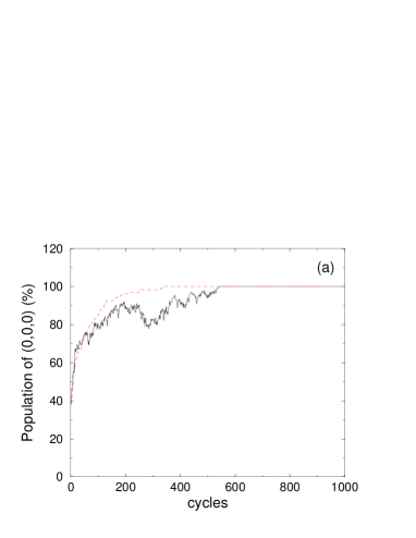
FIG. 2.: Population dynamics of the ground state of the trap for the case of $\eta=2$, $\gamma=0.04\omega$, $\Omega=0.03\omega$, $N=133$, starting from the BED distribution of Fig. 1. (a) Cooling cycles composed of two laser pulses of detunings $\delta=s\omega$, with $s_{1,2}=-4,0$, and $A_{z}=1,-2$ respectively, are used. The non–ideal (solid line) and ideal (dashed line) gas cases are compared. For $\omega=(2\pi)\times 1$kHz the cycle duration is $\sim$ 0.028s. This time can be, however, significantly optimized as discussed in the text. (b) Same case, but only employing pulse $1$.

Let us consider now the case in which collisions are taken into account. We shall consider the same situation and laser–cooling scheme as previously. Fig. 2(a) shows (solid line) the dynamics of the population of the ground-state in presence of collisions. After 600 cycles, all the population is transferred to the ground state of the trap. This means that applying the laser cooling scheme brings the system into an effective BED of $T=0$. It is easy to understand why the effect is maintained in presence of collisions, even considering that the collisional dynamics is much faster than laser–cooling. The laser–cooling mechanism tends to decrease the energy per particle (i.e. the chemical potential of the system), in the same way as evaporative cooling does, but without the losses of particles in the trap during the process. Thermalization via collisions brings the system to a lower temperature. If one repeats the laser cooling sufficiently many times, the system ends with an effective zero temperature. Finally, let us point out that some auxiliary pulses which are needed in the ideal gas case, are not necessary in presence of collisions. In particular, for the previous example, the pulse of zero detuning (required for the ideal gas case, Fig. 2(b) dashed line) is no more needed, as shown in Fig. 2(b) (solid line). Thus, efficient laser–cooling is not only possible in presence of collisions, but it can even be significantly simplified.

We have been limited to rather small $\eta$ due to computational complexity. In particular, in simulations discussed above $\eta=2$ in 3D is considered. The maximal value of $\eta$ we could reach in 3D recently was 4, and the corresponding results are presented in Fig. 3.

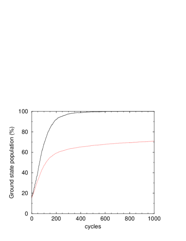
FIG. 3.: Population dynamics of the ground state of the trap for the case of $\eta=4$, $\gamma=0.04\omega$, $\Omega=0.03\omega$, $N=500$, starting from the BED distribution with mean energy 12 $\hbar\omega$. Cooling cycles composed of two laser pulses of detunings $\delta=s\omega$, with $s_{1,2}=-16,0$, and $A_{z}=1,-2$ respectively, are used. The results for noninteracting (dotted line) and interacting (solid line) bosons are presented. For $\omega=(2\pi)\times 1$kHz the cycle duration is $\sim$ 0.028s. This time can be, however, significantly optimized as discussed in the text.

The Monte-Carlo simulations for $\eta=4$ have been performed for 500 atoms occupying 33 3D-energy shells (i. e. 6545 energy levels). The initial mean energy per atom is equal to 12 $\hbar\omega$, which is above the condensation point (mean energy corresponding to $T_{c}$ is about $2.7\hbar\omega$). The initial number of condensed atoms is, however, relatively large (about 10%), what makes the cooling dynamics sufficiently fast from the beginning. The sequence of cooling pulses is similar as in the previous 3D calculations. The first pulse with detuning $\delta=-16\omega$ and $A_{z}=1$ is responsible for confining the atoms, the second one with $\delta=0$ and $A_{z}=-2$ is the dark-state pulse. This combination of pulses is probably not the most efficient in the case of ideal gas, what may be noticed from Fig. 3. After about 200 cycles, the populations of the first excited levels become significantly large. Those levels begin to compete with the ground state and the cooling efficiency is reduced. This effect does not occur in the presence of interactions. The collisions distribute the atoms in more uniform way among the excited states, and the condensation is approached quite fast.

2D and 1D simulations show that same results hold for larger $\eta$. In particular, in 1D we have been able to study the cases up to $\eta=8$, which is illustrated in Fig. 4. For the presented case, the values of parameters are chosen close to the limits of the applicability of our approach. This choice of the parameters leads to shorter cooling times, keeping Festina Lente condition. The pulse length is the same as in the previous simulations, in order to simplify the comparison of the cooling times. The presence of interactions accelerate the cooling process, similarly to the considered 3D examples. The studies for the different values of Lamb-Dicke parameter allowed us to observe that our results scale with $\eta$. In 3D, for instance, keeping $N$ fixed the density scales as $\eta^{-3}$, the three–body loss rate as $\eta^{-6}$, $\omega$ as $\eta^{-2}$, and the cooling time as $\eta^{2}$ times the number of necessary cycles. The estimation of the latter is discussed in Sec. VI.

FIG. 4.: Population dynamics of the ground state of the 1D trap for the case of $\eta=8$, $\gamma=0.5\omega$, $\Omega=0.4\omega$, $N=500$, starting from the BED distribution with mean energy $50\hbar\omega$. Cooling cycles composed of four laser pulses of detunings $\delta=s\omega$, with $s_{1,2,3,4}=-64,-65,37,39$ respectively, are used. The interacting case (solid line) and noninteracting case (dotted line) are compared. For $\omega=(2\pi)\times 1$kHz the cycle duration is $\sim$ 0.056s. This time can be, however, significantly optimized as discussed in the text

IV Rapid thermalization in the weak condensation regime

From the above discussion it is clear that physically it is to be expected that collisions will act on a faster time scale then the laser cooling. In that case, collisions will provide a fast thermalization mechanism. The dynamics of the system will reduce to a fast approach toward instantaneous thermal equilibrium, and a slow change of effective temperature $T$. In order to describe these changes quantitatively, we have to write down explicitly kinetic equations describing populations of the trap levels. This is done, as mentioned above, by performing adiabatic elimination of the excited state, and is discussed in more details below.

In the regime of parameters we consider, the most of the atoms are in the ground state during the dynamics. In particular the system is affected by two different time scales, a slow one given by the commutator with $\hat{H}_{las}$ and other given by the rest of terms in the master equation. Due to this fact we can use adiabatic elimination techniques to remove the excited-state populations. Let $|\vec{n}\rangle\equiv|N_{0},N_{1},\dots;g\rangle$$\otimes|0,0,\dots;e\rangle$ the ground state configurations with $N_{j}$ atoms in the $j$th level, and no excited atoms; let their corresponding energies are $E_{\vec{n}}$, and their corresponding populations $\rho_{\vec{n}\vec{n}}\equiv\langle\vec{n}|\rho|\vec{n}\rangle$. By using standard Projection Operator techniques it is possible to show that the adiabatic elimination of the excited state levels (see Appendix B of the Ref. [19]) leads to a set of rate equations for the populations:

$$\dot{\rho}_{\vec{n}\vec{n}}(t)=\sum_{\vec{m}}P_{\vec{n}\leftarrow\vec{m}}\rho_{\vec{m}\vec{m}}(t)-\sum_{\vec{m}}P_{\vec{m}\leftarrow\vec{n}}\rho_{\vec{n}\vec{n}}(t)+\dot{\rho}^{coll}_{\vec{n}\vec{n}}(t),$$ (18)

where $P_{\vec{m}\leftarrow\vec{n}}$ are also defined in the Appendix of the Ref.[19], and can be understood as the probabilities to undergo a transition from a ground–state configuration: $|\vec{n}\rangle=|N_{0},N_{1},\dots\rangle$ to other configuration $|\vec{m}\rangle$=$|N^{\prime}_{0},N^{\prime}_{1},\dots\rangle$.

The last term in Eq. (18) denotes the collisional contribution of the changes of $\rho_{\vec{n}\vec{n}}(t)$. A detailed discussion of the dynamics introduced by this term can be found in [25, 26]. In our case, we do not have to specify it here: we just have to remember that in the regime of rapid thermalization, this terms leads to a very fast thermalization of the system.

Eq. (18) can be rewritten in terms of rate equations with respect to the populations $N_{j}$ in each level of the ground–state trap:

$$\dot{N}_{n}=\sum_{m}\Gamma_{n\leftarrow m}N_{m}-\sum_{m}\Gamma_{m\leftarrow n}N_{n}+\dot{N}_{n}^{coll},$$ (19)

where the last term on RHS describes the contribution of collisions, while the rates are of the form:

$$\Gamma_{n\leftarrow m}=\frac{\Omega^{2}}{2\gamma}\int_{0}^{2\pi}d\phi\int_{0}^{\pi}d\theta{\cal W}(\theta,\phi)$$ (20)

$$\times\left|\sum_{l}\frac{\gamma\eta_{ln}^{\ast}(\vec{k})\eta_{lm}(k_{L})}{[\delta-\omega(l-m)]+i\gamma R_{ml}}\right|^{2}(N_{n}+1-\delta_{n,m}).$$ (21)

We have approximated here the excited and ground potentials by an harmonic potential of frequency $\omega$, whereas:

$$R_{ml} = \int_{0}^{2\pi}d\phi\int_{0}^{\pi}d\theta{\cal W}(\theta,\phi)$$ (22)

$$\times \sum_{n^{\prime}}|\eta_{ln^{\prime}}(\vec{k})|^{2}(N_{n^{\prime}}+1-\delta_{n^{\prime},m}).$$ (23)

To obtain the rates $\Gamma_{n\leftarrow m}$ we have used the properties of the creation and annihilation operators when applied on Fock states. Note that Eq. (19) is the same as that we have found in [18] for the single–atom case. However, the rates (21) and the single–atom ones are quite different. For the single–atom case they coincide as they should, but for the many–atom case, transition rates (21) become nonlinear, due to their dependence on the number of atoms in each trap level. In particular, we clearly distinguish here the two different quantum–statistical contributions:

• In the denominator of the rates, we observe that the spontaneous emission acquires a collective character (similar as that observed in superradiance).

• In the numerator of the rates, the bosonic–enhancement factor $(N_{n}+1-\delta_{n,m})$ appears.

The bosonic–enhancement factor favors the atoms into just one level of the trap. The reason is that if we are able to pump a significant amount of atoms into one single level $|n\rangle$, subsequent transitions into $|n\rangle$ are more and more probable. Therefore the condensation is more effective.

The contribution of the collective spontaneous emission is unfortunately not so advantageous. The cooling methods designed for the single–atom case, which we want to apply in the many–atom case, are based on resonant processes, and are therefore quite dependent on a narrow resonance. Note that the width of the resonance centered at $\delta=\omega(l-m)$ is given by $\gamma R_{ml}$. If $\gamma R_{ml}$ grows, then the resonance is broadened, and the dark–state effects could cease to exist. On the other hand, as $R_{ml}$ grows, the height of the resonance becomes lower, and consequently the cooling becomes slower. These negative effects can be avoided by using a sufficiently small $\gamma$, which is possible in Raman cooling scheme. In Ref. [19] for instance, the value $\gamma=0.005\omega$ was used in all the calculations, which guaranteed for one–dimensional calculations that only the resonant terms were relevant. It has also been demonstrated that the negative effects are less important for higher dimensions. Note that the decreasing of $\gamma$ makes the cooling slower. In examples of $R_{ml}$’s discussed in [19] it has led to large cooling times (larger than $20$ seconds for sodium atoms). This technical problem can be eventually solved by decreasing externally $\gamma$ during the cooling process, in such a way that the maximum effective collective spontaneous emission rate remains approximately constant and comparable to, say, $\omega/2$. Such technical optimization would increase the cooling rate, allowing for realistic cooling times, as we will show in Section IV.

In the limit of fast thermalization, we can assume that all $N_{n}$ adjust their values to an instantaneous thermal equilibrium characterized by the temperature $T(t)$, i.e. are given by the Bose-Einstein distribution. The temperature varies slowly in time as the laser cooling proceeds. Particularly interesting is the situation below critical temperature, in which we have

$$N_{n}=\exp(-\beta(t)\hbar\omega_{n})/(1-\exp(-\beta(t)\hbar\omega_{n})),$$ (24)

for $n\neq 0$, and

$$N_{0}=N(1-(T(t)/T_{c})^{3}),$$

where $\beta(t)=1/k_{B}T(t)$. The critical temperature is given by

$$k_{B}T_{c}=\hbar\omega(N/g_{3}(1))^{1/3},$$

where the Bose function $g_{3}(1)\simeq 1.2$. From the rate equations (19) we immediately get the equation characterizing the slow changes of the bare energy of the system $E=\sum_{n}\hbar\omega_{n}N_{n}$. Below the condensation point, $E(T)=3k_{B}T(k_{B}T/\hbar\omega)^{3}g_{4}(1)$, where $g_{4}(1)\simeq 1.08$, so that the above Eqs. 19 gives us the desired equation describing the changes of the temperature,

$$\dot{E}=\sum_{n}\hbar\omega_{n}\left[\sum_{m}\Gamma_{n\leftarrow m}N_{m}-\sum_{m}\Gamma_{m\leftarrow n}N_{n}\right].$$ (25)

We can easily rewrite this equation as

$$\frac{dT}{dt}=F(T),$$ (26)

where

$$F(T) = \frac{T}{4E(T)}$$ (27)

$$\times \sum_{n}\hbar\omega_{n}\left[\sum_{m}\Gamma_{n\leftarrow m}N_{m}-\sum_{m}\Gamma_{m\leftarrow n}N_{n}\right].$$ (28)

Assuming that the ground state is perfectly dark, i.e. $\Gamma_{m\leftarrow 0}=0$ for all $m$, it is easy to see that this equation has a (stable) stationary solution $T=0$. If the ground state is not perfectly dark, one obtains a finite stationary value $T_{st}$. The stationary temperature is plotted against $N$ in Fig. 5. If $N$ is sufficiently large $T_{st}$ is very small, as we expect. The cooling rate during approach to $T\simeq 0$ is of the order of typical $\Gamma_{0\leftarrow m}$, and becomes significantly slower only at very low temperatures for very large $N$ (compare the discussion in [19]).

FIG. 5.: Stationary value of the temperature $T_{st}/T_{c}$ as a function of $N$ for the case of $\eta=4$, $\gamma=0.04\omega$, $\Omega=0.03\omega$. The same results in logarithmic scale are presented in the inset.

The value of $T_{st}$ can be estimated assuming that the final distribution of $N_{n}$ will more or less balance the laser cooling dynamics. Similarly as in Ref. [19], we can consider the limit when $N_{0}\simeq N$, $N_{m}\ll N_{0}$ for $m\neq 0$ in a self-consistent way. In that limit the expected stationary values of $N_{m}$ are

$$N_{n}\simeq\Gamma_{n\leftarrow 0}N_{0}/\Gamma_{0\leftarrow n}.$$

We have $\Gamma_{n\leftarrow 0}\sim O(1)$, $\Gamma_{0\leftarrow n}\sim O(N_{0})$, so that $N_{n}\sim O(\gamma/\omega)$ in the stationary state. In this limit, the dynamics consists of independent jumps $0\to n\to 0$ [19], and only the band of $n$’s corresponding to roughly two recoil energies is relevant ($n\leq 2E_{R}/\hbar\omega=2\eta^{2}$). From the expression

$$\sum_{m\neq 0}^{m\leq 2\eta^{2}}N_{m}=N-N_{0},$$

we estimate then

$$\frac{T_{st}}{T_{c}}=\left(\sum_{m\neq 0}^{m\leq 2\eta^{2}}N_{m}/N\right)^{1/3},$$

which implies that $k_{B}T_{st}\simeq k_{B}T_{c}\eta^{2}(\gamma/\omega N)^{1/3}\simeq(\gamma/\omega)^{1/3}E_{R}$. As we see as $N\to\infty$, $T_{st}/T_{c}\to 0$ as $1/N^{1/3}$. This estimation provides in fact only an upper bound for $T_{st}$, due to the fact that it does not take into account Franck-Condon coefficients. Numerical calculations for $\eta=4$, $\gamma=0.04\omega$ and $\Omega=0.03\omega$ presented in Fig. 5 clearly indicates then $T_{st}\rightarrow 0$ even faster as $1/\sqrt{N}$ for $N\rightarrow\infty$. We shall show in the next section that similar conclusions hold beyond the weak condensation.

V Beyond the weak condensation regime

Let us first point out that beyond the weak condensation regime, the mean–field energy cannot be neglected. This has two–fold consequences: (i) The levels of the trap are non–harmonic, i.e. they are not equally separated, because their energies become dependent on the occupation numbers; (ii) the wavefunctions are different, and in particular the condensate wavefunction becomes broader (we consider here only $a>0$). The fact that the energy levels are not harmonic any more, complicates the laser cooling, but the use of pulses with a variable frequency and band–width should produce the same results as those presented here. The point (ii) implies that the central density of the interacting gas is much lower than the one predicted for noninteracting particles, and therefore the dangerous regime of $n\simeq 5\times 10^{14}$ atoms/cm³ is reached for larger number of atoms than in the ideal case. For example, for the case of Magnesium, wavelength $\lambda=600$nm and $\eta=8$, the mentioned density regime is reached for just $N=3.5\times 10^{3}$, whereas in Thomas–Fermi approximation the same is true for $N=6.6\times 10^{5}$. Below this number, the interaction between the particles is dominated by the elastic two–body collisions considered in this paper. We show below that if our laser cooling scheme could be extended beyond the weak–condensation regime, laser–induced condensation of more than $10^{6}$ atoms would be feasible.

In general, to extend the quantum master kinetic theory beyond the weak condensation theory is a formidable task (compare [25, 26]). In general we do not know how the many body states of the trapped gas change in the course of the dynamics. The situation simplifies, however, in the limit of fast thermalization. The collisions assure then that the instantaneous thermal equilibrium is achieved within a fast time scale. Such equilibrium can be very well described for a weakly interacting Bose gas using the Bogoliubov-Hartree-Fock (BHF) theory [21].

A Bogoliubov-Hartree-Fock theory

The BHF theory has various versions; for our purposes perhaps the best approach is the one valid for a fixed number of atoms developed by Gardiner[31], and Castin and Dum [32]. In those approaches one does not break the phase symmetry, and avoid thus the time dependent effects associated with the spreading of the phase distribution [33]. Unfortunately, the number conserving approach is technically tedious. It is therefore easier to use the standard BHF theory, with a broken phase symmetry and in the Popov approximation. In this case we have to neglect the effects of slow spreading of the phase distribution. This approach will be used below. In the standard BHF theory at finite $T$, we introduce the quasi–particle annihilation and creation operators, which are related via the unitary Bogoliubov transform to the atomic quantum field operators [33]:

$$\tilde{g}_{k} = \int d^{3}x\left[u^{*}_{k}(x)\hat{\Psi}(x)+v_{k}(x)\Psi^{{\dagger}}(x)\right],$$ (29)

$$\tilde{g}^{{\dagger}}_{k} = \int d^{3}x\left[u_{k}(x)\hat{\Psi}^{{\dagger}}(x)+v^{*}_{k}(x)\Psi(x)\right],$$ (30)

where $u_{k}$ and $v_{k}$ fulfill the Bogoliubov–de Gennes equations with the eigenenergy $\hbar\tilde{\omega}_{k}$. In particular, $g_{0}$, $g_{0}^{{\dagger}}$ are associated with annihilation or creation of condensed particles. Using the bare states of the trap, the above relation can be rewritten as

$$\tilde{g}_{k} = \sum_{n}\left[u^{*}_{kn}g_{n}+v_{kn}g^{{\dagger}}_{n}\right],$$ (31)

$$\tilde{g}^{{\dagger}}_{k} = \sum_{n}\left[u_{kn}g^{{\dagger}}_{n}+v^{*}_{kn}g_{n}\right],$$ (32)

where $u_{kn}=\int d^{3}x\ u^{*}_{k}(x)\psi_{n}(x)$. The above equations can be inverted to obtain

$$g_{n} = \sum_{k}\left[u_{kn}\tilde{g}_{k}-v_{kn}\tilde{g}^{{\dagger}}_{k}\right],$$ (33)

$$g^{{\dagger}}_{n} = \sum_{k}\left[u^{*}_{kn}\tilde{g}^{{\dagger}}_{k}-v^{*}_{kn}\tilde{g}_{k}\right].$$ (34)

The instantaneous equilibrium corresponds to a thermal state of the system described by the approximated Hamiltonian $\sum_{k}\hbar\tilde{\omega}_{k}\tilde{g}_{k}^{{\dagger}}\tilde{g}_{k}$. In order to describe the cooling dynamics we have to express the quantum master equation of section II in terms of the BHF operators. We need to do it only for the terms responsible for laser cooling, since the collisional and free parts are responsible only for reaching the instantaneous equilibrium. Following the same steps as in previous section, we perform the adiabatic elimination of the excited state, carefully replacing particles by quasiparticles at each step.

B Rate equations for populations

Let $|\vec{n}\rangle\equiv|N_{0},N_{1},\dots;g\rangle$$\otimes|0,0,\dots;e\rangle$ be the ground state configurations with $N_{n}$ quasiparticles in the $n$th level, and no excited atoms; let their corresponding energies are $\tilde{E}_{\vec{n}}$, and their corresponding populations $\rho_{\vec{n}\vec{n}}\equiv\langle\vec{n}|\rho|\vec{n}\rangle$. By using the similar Projection Operator techniques as in the previous section it is possible to show that the adiabatic elimination of the excited state levels leads to a set of rate equations for the populations:

$$\dot{\rho}_{\vec{n}\vec{n}}(t)=\sum_{\vec{m}}P_{\vec{n}\leftarrow\vec{m}}\rho_{\vec{m}\vec{m}}(t)-\sum_{\vec{m}}P_{\vec{m}\leftarrow\vec{n}}\rho_{\vec{n}\vec{n}}(t)+\dot{\rho}^{coll}_{\vec{n}\vec{n}}(t),$$ (35)

where $P_{\vec{m}\leftarrow\vec{n}}$ have similar form as those that appear in the weak condensation limit

$$P_{\vec{n}\leftarrow\vec{m}}=2\gamma\int d\phi d\theta sin\theta{\cal W}(\theta,\phi)\sum_{s,l}$$ (36)

$$\times\left|\langle\vec{n}|(\tilde{\eta}_{ls}^{\ast}(\vec{k})\tilde{g}_{s}^{{\dagger}}+\tilde{\zeta}_{ls}(\vec{k})\tilde{g}_{s})e_{l}\frac{1}{E_{\vec{m}}-\hat{H}_{eff}}\hat{H}_{las}^{(+)}|\vec{m}\rangle\right|^{2},$$ (37)

where $\tilde{\eta}_{ls}(\vec{k})=\int d^{3}x\psi^{*}_{l}(x)e^{i\vec{k}\cdot\vec{x}}u_{s}(x)=\sum_{s^{\prime}}\eta_{ls^{\prime}}u_{ss^{\prime}}$, and $\tilde{\zeta}_{ls}(\vec{k})=\int d^{3}x\psi^{*}_{l}(x)e^{i\vec{k}\cdot\vec{x}}v_{s}(x)=\sum_{s^{\prime}}\eta_{ls^{\prime}}v_{ss^{\prime}}$. The laser Hamiltonian is also reexpressed as

$$\hat{H}_{las}=\frac{\hbar\Omega}{2}\sum_{l,m}e_{l}^{{\dagger}}(\tilde{\eta}_{lm}(k_{L})g_{m}+\tilde{\zeta}^{*}_{lm}(k_{L})g^{{\dagger}}_{m}).$$

As before, the probabilities (37) can be understood as the probabilities to undergo a transition from a ground–state quasi-particle configuration: $|\vec{n}\rangle=|N_{0},N_{1},\dots\rangle$ to other quasi–particle configuration $|\vec{m}\rangle$=$|N^{\prime}_{0},N^{\prime}_{1},\dots\rangle$.

The last term in Eq. (35) denotes the collisional contribution to the changes of $\rho_{\vec{n}\vec{n}}(t)$. We do not have to specify it here: as in Section IV we just have to remember that in the regime considered, this terms leads to a very fast thermalization of the system.

Eq. (35) can be rewritten in terms of rate equations with respect to the quasi–particle populations $N_{n}$ in each level of the ground–state trap:

$$\dot{N}_{n}=\sum_{m}\Gamma_{n\leftarrow m}N_{m}-\sum_{m}\Gamma_{m\leftarrow n}N_{n}+\dot{N}_{n}^{coll},$$ (38)

where the last term on RHS describes the contribution of collisions, while the rates are of the form:

$$\Gamma_{n\leftarrow m}=\frac{\Omega^{2}}{2\gamma}\int_{0}^{2\pi}d\phi\int_{0}^{\pi}d\theta{\cal W}(\theta,\phi)$$ (39)

$$\times\left\{\left|\sum_{l}\frac{\gamma\tilde{\eta}_{ln}^{\ast}(\vec{k})\tilde{\eta}_{lm}(k_{L})}{\delta-\omega^{e}_{l}+\tilde{\omega}_{m}+i(\gamma R_{ml}\!+\!\gamma_{L})}\right|^{2}\!(N_{n}+1-\delta_{n,m})\right.$$ (40)

$$+\left.\left|\sum_{l}\frac{\gamma\tilde{\zeta}_{ln}(\vec{k})\tilde{\zeta}^{*}_{lm}(k_{L})}{\delta-\omega^{e}_{l}-\tilde{\omega}_{m}+i(\gamma R_{ml}\!+\!\gamma_{L})}\right|^{2}\!(N_{n}-\delta_{n,m})\!\right\}$$ (41)

In the above expression we have used rotating wave approximation with respect to quasiparticle frequency spacings. One should stress that, although in general splittings between the quasiparticle energies can be small, in the most interesting limit of large $N$, i.e. in the hydrodynamic regime the quasiparticle spectra are very regular, and the splittings are of the order of the bare harmonic oscillator frequency $\omega$[34]. That is why in the hydrodynamic regime the use of RWA with respect to the quasiparticle energy splittings is very well grounded. The widths in Eq. (41) become now

$$R_{ml} = \int_{0}^{2\pi}d\phi\int_{0}^{\pi}d\theta{\cal W}(\theta,\phi)$$ (42)

$$\times \sum_{n^{\prime}}|\tilde{\eta}_{ln^{\prime}}(\vec{k})|^{2}(N_{n^{\prime}}+1-\delta_{n^{\prime},m})$$ (43)

$$\times \sum_{n^{\prime}}|\tilde{\zeta}_{ln^{\prime}}(\vec{k})|^{2}(N_{n^{\prime}}-\delta_{n^{\prime},m}).$$ (44)

We have additionally included in the expression (41) the width $\gamma_{L}$ which mimics the effects of the laser bandwidth, and which is necessary to assure approximate fulfilling of the resonance conditions. The widths $\gamma_{L}$ should in practice be of the order of $\omega$.

The equations derived in this section have a very similar form to the one derived in the previous sections. In particular, we expect that in the Thomas-Fermi (hydrodynamic) regime, they will lead to the self–consistent equation for the effective temperature. We can easily rewrite this equation as

$$\frac{dT}{dt}=F(T),$$ (45)

where

$$F(T) = \frac{1}{E^{\prime}(T)}$$ (46)

$$\times \sum_{n}\hbar\tilde{\omega}_{n}\left[\sum_{m}\Gamma_{n\leftarrow m}N_{m}-\sum_{m}\Gamma_{m\leftarrow n}N_{n}\right],$$ (47)

where $N_{m}$ are distributed according to the Bose–Einstein distribution corresponding to the quasiparticle Hamiltonian, whereas $E(T)=\sum_{n}\hbar\tilde{\omega}_{n}N_{n}$, $E^{\prime}(T)=dE/dT$. Note that temperature dependence enters the above equations explicitly, and through the dependence of the quasiparticles and their energies on the temperature in the BHF theory at finite $T$. In the limit of large $N$, the same argumentation as in previous section can be applied. We expect that the system will be cooled down to the temperature $T_{st}\simeq 0$, and that the stationary temperature $T_{st}$ will be of the order of $k_{B}T_{st}\simeq k_{B}T_{c}\eta^{2}(\gamma/\omega N)^{1/3}\simeq(\gamma/\omega)^{1/3}E_{R}$. As we see as $N\to\infty$, $T_{st}/T_{c}\to 0$ at least as fast as $1/N^{1/3}$.

VI Prospects for all optical BEC

According to our results the prospects for all optical BEC are very good provided several precautions are realized in experiments. The prescription to achieve all optical BEC is:

• Use a dipole trap of the moderate size $\eta\simeq 2-8$ and $\omega\sim 2\pi\times 1$ kHz.

• Trap and cool atoms into the electronic hyperfine ground state. This allows to eliminate non-elastic two body collisions from considerations.

• Work in the Festina-Lente limit to avoid reabsorptions. Use either natural narrow line, or quenched (Raman) transition of width $\gamma_{eff}<\omega$. In fact to shorten the cooling dynamics try to work with $\gamma_{eff}\sim\omega/2$.

• work with red detuned laser tuned below or in between the molecular resonances to avoid photoassociation losses.

• Avoid high densities, i. e. limit the number of trapped atoms $N$ in such a way that $n<5\cdot 10^{14}/{\rm cm}^{3}$. This will allow you to avoid 3-body losses and remaining photoassociation losses.

In the Tab. I we present our estimates for the maximal number of condensed atoms and the cooling time. We have considered here Mg atoms, and assumed $\lambda_{L}=600$nm and scattering length $a_{sc}\simeq 5$ nm. For various values of $\eta$ we have then calculated corresponding trap frequency $\omega$. Maximal number of atoms $N_{max}$ has been estimated from requirement that the corresponding peak density should be $5\cdot 10^{14}/{\rm cm}^{3}$. The calculations has been done for the ideal ($a_{sc}=0$) and weakly interacting gas, where for simplicity the Thomas-Fermi density profile was assumed.

For the estimation of the cooling time $t_{cool}$ we use the following reasoning. The probability of atom jump (transfer) from level $m$ to level $n$ is proportional to the occupation numbers: $p_{m\rightarrow n}\sim N_{m}(N_{n}+1)$. If we omit the dependence on Frank-Condon coefficients, the jump probability is given by $p_{m\rightarrow n}={\cal N}N_{m}(N_{n}+1)$, where ${\cal N}$ should be determined from the normalization condition: $\sum_{m}\sum_{n}p_{m\rightarrow n}=p_{tot}$, where $p_{tot}$ is total probability of jump. Below we shall assume that in each cycle roughly 10% of atoms undergo a jump, i. e. $p_{tot}\simeq 0.1$. We consider the final stage where only the dark-state pulse for the ground state is responsible for cooling. We assume that the ground state is perfectly dark, i. e. $p_{0\rightarrow m}=0$ for all $m\neq 0$. The spontaneous emission process scatters the atoms within the energy band of width about $4\eta^{2}\hbar\omega=4E_{R}$. Assuming that the dynamics takes place within the region of trap levels with energies smaller than $4\eta^{2}\hbar\omega$, the normalization coefficient reads

$${\cal N}=\frac{p_{tot}}{(N-N_{0})(N+N_{st})}$$ (48)

where $N_{st}$ is the number of states with energies between 0 and $4\eta^{2}\hbar\omega$: $N_{st}\approx(4\eta^{2})^{3}/6$. The cooling efficiency grows if we assume that in each cycle 10% of the excited states population is transferred. This number is consistent with the conditions for the adiabatic elimination used in our derivations. The population of the ground state is increased in every step by $(N-N_{0})\sum_{m\neq 0}p_{m\rightarrow 0}$. Thus we are able to write the formula describing the ground state dynamics:

$$N_{0}(k+1)=N_{0}(k)+\epsilon(N-N_{0}(k))(N_{0}(k)+1),$$ (49)

where $\epsilon=(10(N+N_{st}))^{-1}$ and $k$ labels the cycles. In rough approximation the equation (49) may be replaced by the differential equation

$$\frac{dN_{0}}{dk}=\epsilon(N-N_{0})(N_{0}+1).$$ (50)

Starting with 1 atom in the ground state, the number of cycles needed to obtain $N/2$ condensed atoms may be calculated to be $\ln(N)/(\epsilon N)$. Finally assuming that each cycle have the duration $2/\gamma$, where $\gamma\simeq\omega/4$, we estimate $t_{cool}\simeq 8\ln(N)/(\omega\epsilon N)$. The analytic estimates agree quite well with numerical simulations of Sec. III. Direct inspection of the Tab. I, clearly shows that all-optical BEC of quite large number of atoms should be feasible within a reasonable cooling time.

VII Acknowledgments

We acknowledge support Deutsche Forschungsgemeinschaft (SFB 407), ESF PESC Proposal BEC2000+, and TMR ERBXTCT96-0002. We thank I. Bouchoule, W. Ertmer, E. Rasel, T. Mehlstäubler, J. Keupp, K. Sengstock, and Ch. Salomon for fruitful discussions. We specially acknowledge discussions, help and valuable suggestions from Y. Castin, who took part in the earlier phase of this project.

	$a_{sc}=0$		$a_{sc}=5$nm
$\eta$	$N_{max}$	$t_{cool}$	$N_{max}$	$t_{cool}$
2	55	$119$ms	161	$59.3$ms
4	439	$5.45$s	$1.0\times 10^{4}$	$441$ms
6	$1.4\times 10^{3}$	$51.86$s	$1.2\times 10^{5}$	$1.21$s
8	$3.5\times 10^{3}$	$232.4$s	$6.6\times 10^{5}$	$2.5$s

TABLE I.: Maximal number of condensed atoms and cooling times calculated for Mg atoms, assuming $\lambda_{L}=600$nm and scattering length $a_{sc}\simeq 5$ nm

REFERENCES

- [1] S. Chu, Nobel Lecture, Rev. Mod. Phys. 70, 685 (1998), C. Cohen–Tannoudji, Nobel Lecture, ibid., 707; W. D. Phillips, Nobel Lecture, ibid., 721.
- [2] M. H. Anderson, J. R. Ensher, M. R. Matthews, C. E. Wieman and E. A. Cornell, Science 269, 198 (1995); K.B. Davis, M. O. Mewes, M. R. Andrews, N. J. van Druten, D. S. Durfee, D. M. Kurn and W. Ketterle, Phys. Rev. Lett. 75, 3969 (1995); C. C. Bradley, C. A. Sackett, J. J. Tollett, and R. G. Hulet 75, 1687 (1995); ibid 79, 1170 (1997).
- [3] D. Boiron, A. Michaud, P. Lemonde, Y. Castin, C. Salomon, S. Weyers, K. Szymaniec, L. Cognet and A. Clairon, Phys. Rev. A 53 R3734 (1996).
- [4] M. Rauner, M. Schiffer, S. Kuppens, G. Wokurka, G. Birkl, K. Sengstock, and W. Ertmer, in print in Laser Spectroscopy XIII, (Springer Verlag, Heidelberg, 1997).
- [5] T. Müller–Seydlitz, M. Hartl, B. Breyger, H. Hansel, C. Keller, A. Schnetz, R. J. C. Spreeuw, T. Pfau, and J. Mlynek, Phys. Rev. Lett. 78, 1038 (1997).
- [6] for the recent results see (a) H. Perrin, A. Kuhn, I. Bouchoule and C. Salomon, Europhys. Lett, 42, 395 (1998); (b) H. Katori, T. Ido, Y. Isoya, and M. Kuwata-Gonokami, Phys. Rev. Lett. 82, 1116 (1999); (c) A. J. Kerman, V. Vuletic, Ch. Chin, and S. Chu, Phys. Rev. Lett. 84, 439 (2000);
- [7] J. Lawall, S. Kulin, B. Saubamea, N. Bigelow, M. Leduc, and C. Cohen-Tannoudji, Phys. Rev. Lett. 75, 4194 (1995).
- [8] H. J. Lee, C. S. Adams, M. Kasevich, and S. Chu, Phys. Rev. Lett. 76, 2658 (1996).
- [9] D. W. Sesko, T. G. Walker, and C. E. Wieman, J. Opt. Soc. Am B 8, 946 (1991).
- [10] M. Olshan’ii, Y. Castin, and J. Dalibard, Proceeding of 12th International Conference on Laser Spectroscopy, Eds. M. Inguscio, M. Allegrini, and A. Lasso, (World Scientific, Singapour, 1996).
- [11] A. M. Smith and K. Burnett, J. Opt. Soc. Am. B 9, 1256 (1992).
- [12] K. Esslinger, J. Cooper, and P. Zoller, Phys. Rev. A 49, 3909 (1994).
- [13] One can also use a strongly confining trap with a frequency ; in two atom system the relative role of reabsorption in such a trap can be significantly reduced, see U. Janicke and M. Wilkens, Europhys. Lett. 35, 561 (1996); it is, however, not clear whether this result would hold for many atom systems.
- [14] Y. Castin, J. I. Cirac, and M. Lewenstein, Phys. Rev. Lett. 80, 5305 (1998).
- [15] J. I. Cirac, M. Lewenstein, and P. Zoller, Europhys. Lett. 35, 647 (1996).
- [16] I. Marzoli, J. I. Cirac, R. Blatt and P. Zoller, Phys. Rev. A 49, 2771 (1994).
- [17] G. Morigi, J. I. Cirac, M. Lewenstein and P. Zoller, Europhys. Lett 39, 13 (1997).
- [18] L. Santos and M. Lewenstein, Phys. Rev. A, 59, 613 (1999).
- [19] L. Santos and M. Lewenstein, Eur. Phys. J. D 7, 379 (1999); L. Santos and M. Lewenstein, Phys. Rev. A 60, 3851 (1999);
- [20] L. Santos and M. Lewenstein, Appl. Phys. B 69, 363 (1999);
- [21] For recent reviews of the Bogoliubov–Hartree–Fock see for instance F. Dalfovo, S. Giorgini, L. Pitaevskii, and S. Stringari, Rev. Mod. Phys. 71, 463 (1999); A. Griffin in Proceedings of the International School of Physics “Enrico Fermi” p. 1, Eds. M. Inguscio, S. Stringari and C. E. Wieman, (IOS Press Ohmsa, Amsterdam, 1999); A. L. Fetter, ibid. p. 201; K. Burnett, ibid. p. 265; L. V. Pitaevskii, ibid. p. 287.
- [22] For alkalis, one should apply a static magnetic field to split the levels in the lowest hyperfine manyfold; and are the lowest two Zeeman sublevels. For earth alkalis, must be the ground state, and the excited with the ultranarrow (natural, or laser induced) linewidth.
- [23] Photoassociation losses for laser tuned between resonances, or below the minimum of the molecular potential, become relevant when . For atoms/cm3, . Excited–ground state collisions cause in this case nothing but a modification of the ground state scattering length, see [24].
- [24] P. O. Fedichev, Yu. Kagan, G. V. Shlyapnikov and J. T. M. Walraven, Phys. Rev. Lett. 77, 2913 (1996).
- [25] C. Gardiner and P. Zoller, Phys. Rev. A 55, 2902 (1997).
- [26] D. Jaksch, C. W. Gardiner and P. Zoller, Phys. Rev. A, 56, 575 (1997).
- [27] Consevative dipole–dipole interactions do not play a significant role at the considered densities (cm2), and are omitted in Eq. (9). Their role is discussed in detail in Refs. [19, 20].
- [28] J. Stenger, S. Inouye, M. R. Andrews, H. J. Miesner, D. M. Stamper–Kurn and W. Ketterle, Phys. Rev. Lett. 82, 2422 (1999). In this reference, it is suggested that for the case of the Feshbach resonance at G, it is possible to access the region of zero scattering length without crossing any resonance, and therefore without the inherent three–body losses when crossing.
- [29] M. Marinescu and L. You, Phys. Rev. Lett. 81, 4596 (1998).
- [30] S. L. Cornish, N. R. Claussen, J. L. Roberts, E. A. Cornell, C. E. Wieman, cond-mat/0004290;
- [31] C. W. Gardiner, Phys. Rev. A 56, 1414 (1997).
- [32] Y. Castin, R. Dum, Phys. Rev. A 57, 3008 (1998).
- [33] E. M. Wright, D. F. Walls, J. C. Garrison, Phys. Rev. Lett. 77, 2158 (1996); M. Lewenstein, L. You, Phys. Rev. Lett. 77, 3489 (1996)
- [34] S. Stringari, Phys. Rev. Lett. 77, 2360 (1996); L. You, W. Hoston, and M. Lewenstein, Phys. Rev. A 55, R1581, (1997); L. You, W. Hoston, M. Lewenstein, and M. Marinescu in Proceedings of the International Conference: Quantum Optics IV, Eds. M. Kolwas and J. Mostowski, in special issue of Acta Phys. Polon. A 93, 211 (1998).