HEATING OF TRAPPED PARTICLES CLOSE TO SURFACES — BLACKBODY AND BEYOND

Abstract

We discuss heating and decoherence in traps for ions and neutral particles close to metallic surfaces. We focus on simple trap geometries and compute noise spectra of thermally excited electromagnetic fields. If the trap is located in the near field of the substrate, the field fluctuations are largely increased compared to the level of the blackbody field, leading to much shorter coherence and life times of the trapped atoms. The corresponding time constants are computed for ion traps and magnetic traps. Analytical estimates for the size dependence of the noise spectrum are given. We finally discuss prospects for the coherent transport of matter waves in integrated surface waveguides.

18

Institute of Physics, University of Potsdam, Am Neuen Palais 10, 14469 Potsdam, Germany

10 May 200015 May 2000

1 Introduction

In the field of particle cooling and trapping, a strong trend towards miniaturisation and integration has emerged in the last few years. Small particle traps might form the building blocks of future quantum computers. Integrated atom optical circuits might distribute coherently matter waves for interferometric or nanolithographic applications. Major issues in this field are heating and decoherence that have to be controlled in order to maintain the coherence properties as long as possible. Heating is an intriguing concern because of the dramatic temperature difference between the trapped particles and the macroscopic objects that form a typical miniature trap. In fact, recent experiments with small ion traps have revealed that the life time of the ion’s vibrational ground state gets shorter in smaller traps, making it difficult to down scale the trap geometry to micrometre size [1, 2]. In neutral particle traps, sizes in the micrometre range have already been achieved experimentally [3, 4, 5, 6], but to our knowledge, life times are difficult to measure and are rather limited by background pressure and inelastic few-body collisions.

In this contribution, we consider a simplified geometry for particle traps and compute heating and decoherence rates. The work is divided in two parts. We start with the heating of the vibrational motion of an ion in a tightly confining potential. Using perturbation theory, the heating rate is linked to the cross correlation spectrum of the electric field at the trap center. This noise spectrum is evaluated asymptotically, taking into account that the trap distance is small compared to the photon wave length associated with the ion’s vibration frequency. As a by-product, we also get the noise spectrum for the magnetic field. This spectrum determines the life time of a neutral particle in a magnetic trap, since the fluctuating field induces spin transitions to a non-trapped state, kicking the particle out of the trap. In the second part, we focus on the quasi-free motion of a particle in a wave guide (linear or planar). The particle scatters from thermal field fluctuations and thus loses its spatial coherence. A transport theory is formulated and analytically solved in the limit of a broad-band fluctuation spectrum.

2 Heating of a trapped ion

2.1 Heating rate

Let us focus on a single degree of freedom of the ion’s motion and assume a parabolic confining potential. The Hamiltonian is then simply given by H_trap = ℏΩ( b^†b + 12 ) with $\Omega$ the ion’s vibration frequency (typically in the MHz range). If the ion is perturbed by a time-dependent force, this is described by the potential [7, 8] V(t) = - x ⋅F( r, t ) = - a ^n ⋅F( r, t ) ( b^†+ b ) . We assume that the force varies on a spatial scale much larger than the size $a=(\hbar/(M\Omega))^{1/2}$ of the trap ground state and evaluate it at the trap center ${\bf r}$. ${\bf x}=x\hat{\bf n}$ is the ion’s displacement from the center.

Using standard second-order perturbation theory, one may easily derive a master equation for the reduced density matrix of the ion, that describes its dynamics when the fluctuations of the force field ${\bf F}({\bf r},t)$ are traced over [7, 8, 1, 9]. This master equation allows to derive the equation of motion for the population of the lowest trap levels, as well as for the average creation operator and the average excitation number (in the absence of cooling processes)

$$\dot{\rho}_{00} = -\gamma_{-}\rho_{00}+\gamma_{+}\rho_{11}$$ (1)

$$\langle\dot{n}\rangle = -(\gamma_{+}-\gamma_{-})\langle n\rangle+\gamma_{-}$$ (2)

$$\langle\dot{b}\rangle = -i\Omega\langle b\rangle-\frac{1}{2}(\gamma_{+}-\gamma_{-})\langle b\rangle$$ (3)

The rates $\gamma_{\pm}$ in these formulas are related to the cross spectral density of the force fluctations as follows

$$\gamma_{\pm} = \gamma({\bf r};\pm\Omega)$$ (4)

$$= \frac{a^{2}}{\hbar^{2}}\sum_{i,j}\hat{n}_{i}\hat{n}_{j}S_{F}^{ij}({\bf r};\pm\Omega)$$

with S_F^ij( r; ω) = ∫_-∞^+∞ ​ dτ  ⟨F_i( r, t + τ) F_j( r, t ) ⟩e^i ωτ According to (1), the heating rate from the trap ground state is thus given by $\Gamma_{0\to 1}({\bf r})=\gamma_{-}$. We are thus left with the calculation of the spectral density (2.1) for the perturbing force.

2.2 Electric field noise spectrum

The trapped ion being charged, it is perturbed by fluctuating electric fields, ${\bf F}=q{\bf E}$. The Planck blackbody spectrum then gives the following spectral density S_F^ij( r; ω) = q^2 S_E( ω) δ^ij = q2ℏω3δij3 πε0c3( 1 - e-ℏω/ kBT ) where $T$ is temperature. One must keep in mind, however, that this gives the thermal spectrum only in free space, far from the sources. But the ion is trapped at a distance $z$ from the trap electrodes that is typically much smaller than the photon wave length $\lambda=2\pi c/\Omega$ associated with the vibration frequency. It is thus located in the near field of the electrodes, and the Planck formula does not cover this case. This was recognised already in the early days of ion trapping when ‘hot’ ion clouds (with temperatures much larger than room temperature) were cooled down by thermalisation with the surrounding electrodes, the coupling being provided by the absorption of the electric fields radiated by the moving ions in the lossy metallic environment [10]. When laser cooling took over to reach temperatures in the $\mu$K range, voltage fluctuations due to electric losses became a source of heating. Modeling the ion trap as a lumped circuit with resistance $R(\omega)$, the standard Nyquist formula for Johnson noise gives an electric field spectrum [7, 8, 10] S_F( r; ω) ≈q2kBT R(ω) z2 where the high-temperature limit $k_{B}T\gg\hbar|\omega|$ has been assumed. For a given trap geometry, it is not easy to determine the resistance $R(\omega)$ that enters this formula. Assuming that the electric currents propagate only in the skin layer of the electrodes, the NIST group estimated that the spectrum (2.2) actually gives a heating rate too small to account for the experimental observations. In addition, there are indications that the scaling law $\Gamma_{0\to 1}({\bf r})\propto S_{F}({\bf r})\propto 1/z^{2}$ is not followed experimentally (although it is difficult to exclude other influences when down-scaling the trap geometry) [2].

We now outline a microscopic effective model [11, 9, 2] that may in principle allow to compute the electric noise spectrum for an arbitrary trap geometry.

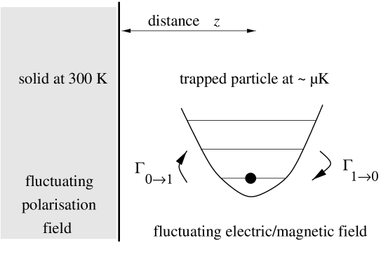
Figure 1: Fig. 1. Sketch of the microscopic effective model used to compute the electric field noise spectrum.

We describe the electric properties of the surrounding metal by its frequency-dependent complex dielectric function $\varepsilon({\bf r};\omega)$. The microscopic source of Johnson noise are fluctuating polarisation fields ${\bf P}({\bf r},t)$ that are thermally excited in the metal. According to the fluctuation dissipation theorem, the spectral density of this fluctuating polarisation is related to the imaginary part of the dielectric function [12, 13, 14]: S_P^ij( r’, r; ω) = 2 ℏε0Im ε( r; ω) 1 - e- ℏω/ kBT δ^ij δ( r’ - r ) Maxwell’s equations now determine the field radiated by this polarisation. It may be written as an integral over the Green tensor E_i( r; ω) = ∫​dr’ ∑_j G^ij( r, r’; ω) P_j( r’; ω) where $G^{ij}$ depends on the geometry of the trap electrodes.

To proceed with the calculation, we now fix the geometry and consider a trap located at a distance $z$ above an infinite flat metallic surface. In this geometry, the Green function in (1) is explicitly known in spatial Fourier space, and it is possible to perform an asymptotic expansion in the near field limit $z\ll\lambda$. As a result, we obtain the following interpolation formula [2, 9] S_E^ij( z ; ω) ≈ℏω  ϱ4 π( 1 - e- ℏω/ kBT )   z3 ( s^ij + δ^ij z δ( ω) ) . As expected, the spectrum only depends on the $distance$ from the surface. The material properties enter through the specific resistance $\varrho$ and the skin depth $\delta(\omega)=c\sqrt{\varepsilon_{0}\varrho/\omega}$. The geometry enters through the power law $S_{E}(z)\propto 1/z^{3}$ in the ‘extreme near field’ $z\ll\delta$. This behaviour may be understood from the principle of detailed balance: the heating rate of the ion is equal to the relaxation rate of an oscillating electric dipole, and it is well known that close to a metallic surface, this rate is dominated by nonradiative transfer and increases as $1/z^{3}$ [15, 16].

We may also extract from (1) an ‘effective resistance’: if the distance is large compared to the skin depth, the near field spectrum indeed follows a $1/z^{2}$ power law, as in eq.(2.2). The comparison yields an effective resistance $R_{\rm eff}(\omega)\approx 3\varrho/(4\pi\delta(\omega))$. This indicates that the thermal currents actually flow in a skin layer right below to the metallic surface, in agreement with the estimates made by the NIST group [1].

The ion heating rate obtained from the spectrum (1) is plotted in figure 2.

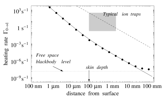
Figure 2: Fig. 2. Heating rate for a trapped ion (mass $40\,$amu, charge $q=e$) trapped in a harmonic trap (frequency $\Omega/2\pi=1\,$MHz) above a copper surface at $300\,$K. Dots: exact evaluation of the electric near field fluctations; solid line: asymptotic expansion (1); dashed line: heating rate from the Johnson noise spectrum (2.2) with $R(\omega)=1\,\Omega$.

We observe that the electric near field fluctuates at a noise level much larger than the blackbody field (dotted line). It is also apparent that life times shorter than 1 s are to be expected when the trap size gets into the micrometre range. The figure also shows that the life times in current traps are not limited by the near field fluctuations discussed here, the observed heating rates being much larger. The NIST group proposed a model including fluctuating electric patch potentials that may explain this discrepancy, but little is known about the dielectric properties of these electric surface domains in the relevant frequency range [2]. In view of recent theoretical and experimental investigations [1, 2, 9, 11, 17, 18], a detailed understanding of ion heating processes is still lacking.

2.3 Magnetic field noise spectrum

To conclude this section, we turn to a different type of trap: a static inhomogeneous magnetic field that traps a paramagnetic atom at local minima of the magnetic field strength. Such traps are routinely used for evaporative cooling [19], and miniature versions close to wires or surfaces have been proposed [6, 20] and actually realised [21, 22, 23, 24, 25]. Thermally fluctuating magnetic fields now may flip the atomic spin, leaving the atom possibly in an unbound potential (see figure 3).

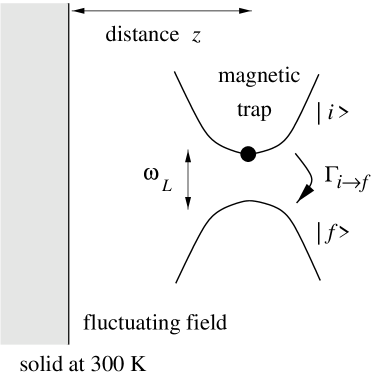
Figure 3: Fig. 3. Fluctuating magnetic fields flip the spin of an atom in a magnetic trap and put it onto a non-trapping potential surface.

The spin flip rate is easily obtained from perturbation theory and relates to the spectral density of the magnetic field fluctuations: Γ_i→f( r ) = 1 ℏ2 ∑_α, β ⟨i — μ_α— f ⟩⟨f — μ_β— i ⟩S^αβ_B( r; ω_L ) where $\omega_{L}=\mu B_{\rm trap}({\bf r})/\hbar$ is the Larmor frequency. The magnetic field spectrum may be calculated using the theory outlined above, and one finds the following asymptotic result [9]: S^αβ_B( z; ω) ≈ℏω  sαβ16 πε02c4ϱ  ( 1 - e- ℏω/ kBT )  z ( 1 + 2 z33 δ3( ω) )^-1 For a spin 1/2 particle, we thus get the trap loss rate shown in figure 4.

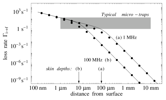
Figure 4: Fig. 4. Spin flip rate (loss rate) for a paramagnetic atom (magnetic moment $\mu=\mu_{B}$) in a magnetic trap above a copper surface at $300\,$K. The Larmor frequency takes the values $\omega_{L}/2\pi=1\,$MHz (curve (a)) and $100\,$MHz (curve (b)). The rate obtained from the blackbody spectrum is much smaller (about $10^{13}\,{\rm s}^{-1}$ for $\omega_{L}/2\pi=100\,$MHz).

We note that in micrometre size traps, the life time is limited to less than a second due to near field fluctuations, which should be an observable effect in current experiments.

3 Decoherence in wave guides

We now turn to the influence of fluctuating near fields on the quasi-free motion of atoms in linear or planar wave guides [4, 6, 20, 21, 25]. The atomic matter wave is scattered from spatial inhomogeneities of the perturbing field, thus changing its momentum. We assume again a statistical description of the scattering process. The typical momentum transfer is thus of the order of $\hbar/\ell$ where $\ell$ is the correlation length of the field. Energy is not conserved because the field is fluctuating, and the maximum energy transfer is roughly limited by $k_{B}T$. Note that this is typically much larger than the kinetic energies involved in cold atomic clouds.

3.1 Transport equation

We want to characterise the evolution of the single-particle spatial density matrix (or coherence function) ρ( r; s ) = ⟨ψ^*( r + 12 s )   ψ( r - 12 s ) ⟩ where the average $\langle\ldots\rangle$ is taken over the spatial and temporal fluctuations of a perturbing potential $V({\bf r},t)$. It is useful to introduce the Wigner transform of the density matrix W( r, p ) = ∫​ d3s 2 πℏ e^ i p ⋅s / ℏ ρ( r; s ) that may be interpreted as a quasi-probability distribution in phase space.

Using second-order perturbation theory, assuming gaussian statistics for the perturbing potential and doing a multiple-scale expansion of the Bethe-Salpeter equation for the coherence function, we get the following transport equation [26]:

$$\Bigl{(}\partial_{t}+\frac{1}{m}{\bf p}\cdot\nabla_{\bf r}+{\bf F}_{\rm ext}\cdot\nabla_{\bf p}\Bigr{)}W({\bf r},{\bf p})=$$

$$\int\!{\rm d}^{D}p^{\prime}\,S_{V}({\bf p}^{\prime}-{\bf p};E_{p^{\prime}}-E_{p})\left[W({\bf r},{\bf p}^{\prime})-W({\bf r},{\bf p})\right]$$ (5)

where $D=1,2$ is the dimension of the wave guide and $S({\bf q};\Delta E)$ the spectral density of the fluctuating potential S_V( q; ΔE) = 1 ℏ2 ∫​dDs   dτ(2πℏ)D ⟨V( r + s, t + τ)   V( r, t ) ⟩  e^ - i ( q⋅s - ΔE τ) / ℏ . We have assumed that the potential is statistically stationary in both space and time.

The left hand side of the transport equation (5) describes the ballistic motion of the atom subject to the external (deterministic) force ${\bf F}_{\rm ext}$. The right hand side describes the scattering off the fluctuating potential. As a function of the momentum transfer $\bf q$, e.g., the spectral density $S_{V}({\bf q};\Delta E)$ is proportional to the spatial Fourier transform of the potential, as to be expected from the Born approximation for the scattering process ${\bf p}\to{\bf p}^{\prime}={\bf p}+{\bf q}$. The transport equation thus combines in a self-consistent way ballistic motion and scattering processes.

3.2 Example: magnetic perturbation

For illustration purposes, we show in figure 5 the magnetic near field spectrum at a distance $z=1\,\mu$m above a flat metallic surface. This spectrum is proportional to $S_{V}({\bf q};\Delta E)$ in (5) for a planar magnetic waveguide.

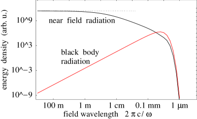
Figure 5: Fig. 5. Magnetic field spectrum vs. frequency at distance $1\,\mu$m above at copper surface at $300\,$K. The frequency $\omega$ is expressed via the electromagnetic wave length $\lambda=2\pi c/\omega$. Note: a kinetic energy of $10\,\mu$K corresponds to a wave length $14\,$km.

One observes that for typical kinetic energies of cold atoms, the magnetic spectrum is essentially flat. In the following, we shall hence approximate the perturbing field by a white noise.

In figure 6,

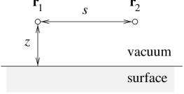
Figure 6: Fig. 6. Spatial (normalised) correlation function of the thermal magnetic near field above a metallic surface at frequency $\omega/2\pi=30\,$MHz. The separation $s$ gives the distance between two observations points at the same height $z$ above the surface. The other parameters are identical to the previous figure 5. Dots: exact evaluation, solid lines: asymptotic expansions in the short-distance regime. For even lower frequencies, the correlation function is essentially unchanged.

we show the normalised spatial correlation function of the thermal magnetic field above a metallic surface. One observes that in a planar wave guide above the surface, the field’s spatial correlation length is of the order of the height $z$. The correlations decay algebraically with the lateral separation $s$ (measured in the waveguide plane parallel to the surface).

3.3 Analytic solution of the transport equation

For a broad band spectrum of the perturbation, we may neglect the dependence of $S_{V}({\bf q},\Delta E)$ on $\Delta E$. The transport equation (5) then simplifies because the integration over the scattered momentum ${\bf p}^{\prime}$ is not restricted by energy conservation. Taking the Fourier transform with respect to both variables ${\bf r}$ and ${\bf p}$ (with conjugate variables ${\bf k}$ and ${\bf s}$), it is simple to derive the following solution

$$\tilde{W}({\bf k},{\bf s};t)=\tilde{W}_{0}({\bf k},{\bf s}-\hbar{\bf k}t/m)\,{\rm e}^{-{\rm i}{\bf F}_{\rm ext}\cdot{\bf s}t/\hbar}\times{}$$

$${}\times\exp{\left[-\gamma\int_{0}^{t}\!\!\left(1-C({\bf s}-\hbar{\bf k}t^{\prime}/m)\right)\!{\rm d}t^{\prime}\right]}$$ (6)

Here, $\tilde{W}_{0}({\bf k},{\bf s})$ is the double Fourier transform of the Wigner function at initial time $t=0$, and $\gamma$ and the normalised spatial correlation function $C({\bf s})$ are related to the correlation function of the perturbation by γC( s ) = 1 ℏ2 ∫_-∞^+∞​dτ  ⟨V( s, τ)   V( 0, 0 ) ⟩, C( 0 ) = 1. We also note that $\gamma$ is the scattering rate $\gamma({\bf p}\to{\bf p}^{\prime})$ for ‘forward scattering’ processes where the final momentum ${\bf p}^{\prime}$ approaches the initial ${\bf p}$. For a magnetic wave guide above a metallic surface, the rate $\gamma$ is essentially of the same order of magnitude as the spin flip rate shown in figure 4.

From the analytic solution (6), it is easily checked that in the absence of the perturbation , the spatial width $\delta r^{2}(t)$ of a cloud increases ballistically according to $\delta r^{2}(t)=\delta p^{2}(0)\,t^{2}/m^{2}$ where $\delta p(0)$ is the initial width of the cloud in momentum space (this latter width remains constant in this case, of course).

3.4 Discussion

Spatial decoherence.

More interesting information may be obtained for a nonzero scattering rate $\gamma$. Note that the spatially averaged atomic coherence function is given by Γ( s ) = ∫​d^Dr   ρ( r; s ) = ~W( k = 0, s ) The solution (6) therefore implies that the spatial coherence decays exponentially with time: Γ( s; t ) = Γ_0( s ) exp[ - γt (1 - C( s ) ) - i F ⋅s  t / ℏ] The decoherence rate depends on the spatial separation between the points where the atomic wave function is probed, and is given by $\gamma({\bf s})=\gamma(1-C({\bf s}))$. It hence saturates to the value $\gamma$ at large separations and decreases to zero for ${\bf s}\to{\bf 0}$. The decay of the coherence function (3.4) is illustrated in figure 7.

Figure 7: Fig. 7. Illustration of spatial decoherence in an atomic wave guide. The spatially averaged coherence function $\Gamma({\bf s},t)$ is plotted vs. the separation ${\bf s}$ for a few times $t$. Space is scaled to the field correlation length $\ell$ and time to the scattering time $1/\gamma$. A Lorentzian correlation function for the perturbation is assumed.

One observes that at time scales $t\geq 1/\gamma$, the spatial coherence is reduced to a coherence length $\xi_{\rm coh}\sim\ell$. After a few collisions with the fluctuating magnetic field, the long-scale coherence of the atomic wave function is thus lost and persists only over scales smaller than the field’s correlation length (where different points of the wave function ‘see’ essentially the same fluctuations). For larger times $t\gg 1/\gamma$, decoherence proceeds at a smaller rate that is related to momentum diffusion, as we shall see now.

Momentum diffusion at long times.

The behaviour of the atomic momentum distribution at long times may be extracted from an expansion of the analytic solution (3.4) for small values of ${\bf s}$. Assuming a quadratic dependence of the field’s correlation function, $C({\bf s})\approx 1-s^{2}/\ell^{2}$, as one would expect for Lorentzian correlations, we find that the atomic momentum distribution is gaussian at long times; it is centered at ${\bf p}_{0}+{\bf F}_{\rm ext}t$ due to the external force, and its width increases according to a diffusion process in momentum space δp^2(t) ≈δp^2(0) + ℏ2γt ℓ2 This was to be expected: the atoms perform a random walk in momentum space, exchanging a momentum of order $\hbar/\ell$ per scattering time $1/\gamma$. The momentum diffusion coefficient $D_{p}=\hbar^{2}\gamma/\ell^{2}$ that may be read off from (3.4) is consistent with this intuitive interpretation. Physically speaking, the atomic cloud is ‘heated up’ due to the scattering from the fluctuating potential. We note that the rate of change of the atomic kinetic energy in the wave guide plane is the same as the one for the tightly bound motion perpendicular to the metallic surface (see [9] for a calculation of this rate).

Translating the width of the momentum distribution into a spatial coherence length, we find a power-law decay at long times, $\xi_{\rm coh}=\ell/\sqrt{\gamma t}$. Finally, a similar calculation yields the width of the atomic cloud in position space: it increases ‘super-ballistically’ at long times, $\delta r^{2}(t)\propto t^{3}$, as a consequence of heating.

4 Conclusion

Particles in small traps close to macroscopic bodies are subject to fluctuating near fields that show noise spectra orders of magnitude above the blackbody level. This is because the geometric distances involved are typically much smaller than the electromagnetic wave lengths associated with the relevant frequencies. As a consequence, the ground state of the vibrational motion of trapped ions is unstable, and coherences between different oscillator levels decay. We have developed a theoretical framework to compute the corresponding heating and decay rates. As a second consequence, quasi-free matter waves in a linear or planar wave guide in the vicinity of macroscopic bodies (substrates or wires) are scattered and lose their spatial coherence. We have identified the relevant time scale and obtained analytic estimates for the behaviour of the atomic coherence function at large spatial and temporal scales. These estimates should be useful, we hope, to design integrated atom optical circuits with controlled decoherence.

Questions that could be addressed in the future pertain to detailed theories for trapped ion heating, as well as to transport processes for condensed atomic samples. Finally, the inclusion of interference effects in multiple scattering might provide a link to study weak and/or strong localisation of matter waves in wave guides.

Acknowledgments. C.H. would like to thank R. Carminati and K. Joulain of the group of J.-J. Greffet at Ecole Centrale (Paris) for useful discussions. Furthermore, D. Leibfried, E. Peik, F. Schmidt-Kaler, J. Schmiedmayer, and J. von Zanthier communicated precious hints on experimental issues.

References

- [1] D. J. Wineland, C. Monroe, W. M. Itano, D. Leibfried, B. E. King, D. M. Meekhof: J. Res. Natl. Inst. Stand. Technol. 103 (1998) 259 [quant-ph/9710025]
- [2] Q. A. Turchette, et al.: Phys. Rev. A (2000), submitted [quant-ph/0002040]
- [3] Y. B. Ovchinnikov, I. Manek, R. Grimm: Phys. Rev. Lett. 79 (1997) 2225
- [4] H. Gauck, M. Hartl, D. Schneble, H. Schnitzler, T. Pfau, J. Mlynek: Phys. Rev. Lett. 81 (1998) 5298
- [5] J. Fortagh, A. Grossmann, C. Zimmermann, T. W. Hänsch: Phys. Rev. Lett. 81 (1998) 5310
- [6] E. A. Hinds, M. G. Boshier, I. G. Hughes: Phys. Rev. Lett. 80 (1998) 645
- [7] S. K. Lamoreaux: Phys. Rev. A 56 (1997) 4970
- [8] D. F. V. James: Phys. Rev. Lett. 81 (1998) 317 [quant-ph/9804048]
- [9] C. Henkel, S. Pötting, M. Wilkens: Appl. Phys. B 69 (1999) 379 [quant-ph/9906128]
- [10] D. J. Wineland, H. G. Dehmelt: J. Appl. Ph. 46 (1975) 919
- [11] C. Henkel, M. Wilkens: Europhys. Lett. 47 (1999) 414 [quant-ph/9902009]
- [12] E. M. Lifshitz: Soviet Phys. JETP 2 (1956) 73 [J. Exper. Theoret. Phys. USSR 29, 94 (1955)]
- [13] B. Huttner, S. M. Barnett: Europhys. Lett. 18 (1992) 487
- [14] H. T. Dung, L. Knöll, D.-G. Welsch: Phys. Rev. A 57 (1998) 3931 [quant-ph/9711039]
- [15] K. H. Drexhage: in Progress in Optics XII (North-Holland, Amsterdam, 1974, pp. 163–232), edited by E. Wolf
- [16] S. Scheel, L. Knöll, D.-G. Welsch: Phys. Rev. A 60 (1999) 4094 [quant-ph/9904015]
- [17] M. Murao, P. Knight: Phys. Rev. A 58 (1998) 663 [quant-ph/9803041]
- [18] S. Schneider, G. J. Milburn: Phys. Rev. A 57 (1998) 3748 [quant-ph/9710044]
- [19] W. Petrich, M. H. Anderson, J. R. Ensher, E. A. Cornell: Phys. Rev. Lett. 74 (1995) 3352
- [20] J. Schmiedmayer: Phys. Rev. A 52 (1995) R13
- [21] J. Denschlag, D. Cassettari, J. Schmiedmayer: Phys. Rev. Lett. 82 (1998) 2014 [quant-ph/9809076]
- [22] J. Reichel, W. Hänsel, T. W. Hänsch: Phys. Rev. Lett. 83 (1999) 3398
- [23] D. Müller, D. Z. Anderson, R. J. Grow, P. D. D. Schwindt, E. A. Cornell: Phys. Rev. Lett. 83 (1999) 5194
- [24] N. H. Dekker, C. S. Lee, V. Lorent, J. H. Thywissen, S. P. Smith, M. Drndić, R. M. Westervelt, M. Prentiss: Phys. Rev. Lett. 84 (2000) 1124
- [25] M. Key, I. G. Hughes, W. Rooijakkers, B. E. Sauer, E. A. Hinds, D. J. Richardson, P. G. Kazansky: Phys. Rev. Lett. 84 (2000) 1371
- [26] L. Ryzhik, G. Papanicolaou, J. B. Keller: Wave Motion 24 (1996) 327