Quantum dynamics and statistics of two coupled down-conversion processes

Abstract

In the framework of Heisenberg-Langevin theory the dynamical and statistical effects arising from the linear interaction of two nondegenerate down-conversion processes are investigated. Using the strong-pumping approximation the analytical solution of equations of motion is calculated. The phenomena reminiscent of Zeno and anti-Zeno effects are examined. The possibility of phase-controlled and mismatch-controlled switching is illustrated.

1 Introduction

Optical parametric processes yield a wide variety of optical phenomena. It is not surprising that many new phenomena will arise if a parametric process is coupled to another one or to a different optical process. For instance, the superposition of signal photons originating from two down-convertors with aligned idler beams leads to nontrivial quantum interference effects [1]. Parametric process coupled via Kerr interaction to an auxiliary mode, exhibiting quantum Zeno effect is another nice example [2, 3]. Many such composite systems (usually called nonlinear couplers) has thoroughly been studied in the literature. All-optical switching in the assymetric nonlinear coupler operating by the second-harmonic generation has been investigated in [4] and its non-classical behaviour has been discussed in [5, 6]. The quantum dynamics and statistics of the symmetric coupler containing two second-harmonic processes have been examined in [7]. The coupler composed of one linear waveguide and one nonlinear waveguide operating by the down-coversion process has been investigated in [8] from the point of view of all optical switching. The occurrence of quantum Zeno and anti-Zeno effects in a similar device has been reported in [10]. Amplitude behaviour of two linearly coupled down-conversion processes has been studied in [8]. Short-length analysis of this device has been given in [9].

In this paper we deal with interesting phenomena arising as a consequence of linear interaction between beams propagating through the symmetric nonlinear coupler, which is composed of two nonlinear waveguides based on the down-conversion processes. In fact this arrangement can be looked at as a continuous version of famous Mandel’s experiment [1], involving real physical interaction between the two down-conversion processes. In Section 2 the equations of motion are derived and their analytical solutions are given. Sections 3 and 4 are devoted to the study of quantum dynamics and statistics of the coupler. Its non-classical properties are discussed in Section 5.

Figure 1: Sketch of symmetric nonlinear coupler formed from two nonlinear waveguides with susceptibility $\chi^{(2)}$. The interacting beams are described by annihilation operators; $L$ is the interaction length.

2 Equations of motion and their solution

The coupler which is investigated in this article is composed of two nonlinear waveguides operating by the down-conversion processes in a directional arrangement (see Fig. 1). The linear energy exchange by means of evanescent waves between pump, signal and idler beams is considered. The nonlinear media are assumed to be lossy. If such a system is far from resonance, the effective description involving only the field variables is adequate [11]. The effective momentum operator then reads

$$\hat{G}=\hat{G}_{1}+\hat{G}_{2}+\hat{G}_{res.}+\hat{G}_{res.-syst.}+\hat{G}_{int.},$$ (1)

where

$$\hat{G}_{i} = \hbar\sum_{j={P_{i}},{S_{i}},{I_{i}}}k_{j}\hat{a}_{j}^{{\dagger}}\hat{a}_{j}+\hbar\left(\Gamma_{i}\hat{a}_{P_{i}}\hat{a}_{S_{i}}^{{\dagger}}\hat{a}_{I_{i}}^{{\dagger}}+\mbox{h.c.}\right)\mbox{\qquad{for\quad{i=1,2}}},$$

$$\hat{G}_{res.} = \hbar\sum_{i=1}^{2}\sum_{j={P_{i}},{S_{i}},{I_{i}}}\sum_{l}k_{lj}\hat{b}_{lj}^{{\dagger}}\hat{b}_{lj},$$

$$\hat{G}_{res.-syst.} = -\hbar\sum_{i=1}^{2}\sum_{j={P_{i}},{S_{i}},{I_{i}}}\sum_{l}\left(\kappa_{lj}\hat{a}_{j}\hat{b}_{lj}^{{\dagger}}+\mbox{h.c.}\right),$$

$$\hat{G}_{int.} = \hbar(\kappa_{P}\hat{a}_{P_{1}}\hat{a}_{P_{2}}^{{\dagger}}+\kappa_{S}\hat{a}_{S_{1}}\hat{a}_{S_{2}}^{{\dagger}}+\kappa_{I}\hat{a}_{I_{1}}\hat{a}_{I_{2}}^{{\dagger}}+\mbox{h.c.}),\$$ (2)

where $\hat{a}_{j}({\hat{a}_{j}}^{{\dagger}})$, $j=P_{1},P_{2},S_{1},S_{2},I_{1},I_{2}$ are annihilation (creation) operators of pump, signal, and idler modes. Corresponding wavevectors along the z-axis of propagation are $k_{P_{1}}$, $k_{P_{2}}$, $k_{S_{1}}$, $k_{S_{2}}$, $k_{I_{1}}$ and $k_{I_{2}}$. Linear coupling constants between pump, signal and idler modes are denoted $\kappa_{P}$, $\kappa_{S}$ and $\kappa_{I}$. Nonlinear coupling constants are denoted as $\Gamma_{1}$ and $\Gamma_{2}$. Each mode $j$ is coupled via linear coupling constant $\kappa_{lj}$ to the $l$-th reservoir mode characterized by annihilation (creation) operators $\hat{b}_{lj}({\hat{b}_{lj}}^{{\dagger}})$ and wavevector $k_{lj}$ along z-axis of propagation. The symbol $\hbar$ denotes the reduced Planck constant and h.c. represents Hermitian conjugate terms.

The model represented by the momentum operator (1) is symmetric both under the exchange $1\leftrightarrow 2$, $\kappa_{P}\leftrightarrow\kappa_{P}^{\ast}$, $\kappa_{S}\leftrightarrow\kappa_{S}^{\ast}$, $\kappa_{I}\leftrightarrow\kappa_{I}^{\ast}$ and under the exchange $S\leftrightarrow I$. Since the dynamical behaviour of the system is completely determined by its momentum operator, the symmetries are conserved during evolution. This is convenient because it is not necessary to write down all calculated quantities, the rest being simply obtained by the above mentioned exchanges.

Substituting (1) into the Heisenberg equations of motion $(i\hbar\frac{d}{dz}\hat{a}=[\hat{G},\hat{a}])$, introducing slowly varying operators $\hat{A}_{j}(z)=\hat{a}_{j}(z)\mbox{exp}(-ik_{j}z)$ and applying the Wigner-Weisskopf approximation [12], we arrive at the following Heisenberg-Langevin equations of motion

$$\frac{d\hat{A}_{P_{1}}}{dz} = -\gamma_{P_{1}}\hat{A}_{P_{1}}+i{\kappa}_{P}^{\ast}\hat{A}_{P_{2}}\mbox{exp}(-i\Delta k_{P}z)+i{\Gamma}_{1}^{\ast}\hat{A}_{S_{1}}\hat{A}_{I_{1}}\mbox{exp}(-i\Delta l_{1}z)+\hat{L}_{P_{1}}(z),$$

$$\frac{d\hat{A}_{S_{1}}}{dz} = -\gamma_{S_{1}}\hat{A}_{S_{1}}+i{\kappa}_{S}^{\ast}\hat{A}_{S_{2}}\mbox{exp}(-i\Delta k_{S}z)+i\Gamma_{1}\hat{A}_{P_{1}}\hat{A}_{I_{1}}^{\dagger}\mbox{exp}(i\Delta l_{1}z)+\hat{L}_{S_{1}}(z),$$

where $\Delta k_{k}=k_{k_{1}}-k_{k_{2}}$, $k=P,S,I$ are linear mismatches, $\Delta l_{i}=k_{P_{i}}-k_{S_{i}}-k_{I_{i}}$, $i=1,2$ are nonlinear mismatches, $\gamma_{j}$, $j=P_{1},P_{2},S_{1},S_{2},I_{1},I_{2}$ are damping contants and the Langevin forces $\hat{L}_{j}(z)$ are assumed to be Markoffian

$$\langle\hat{L}_{j}(z)\rangle = \langle\hat{L}_{j}^{\dagger}(z)\rangle=\langle\hat{L}_{j}(z)\hat{L}_{k}(z^{\prime})\rangle=0,$$

$$\langle\hat{L}_{j}^{\dagger}(z)\hat{L}_{k}(z^{\prime})\rangle = 2\gamma_{j}\langle n_{dj}\rangle\delta_{jk}\delta(z-z^{\prime}),$$

$$\langle\hat{L}_{j}(z)\hat{L}_{k}^{\dagger}(z^{\prime})\rangle = 2\gamma_{j}(\langle n_{dj}\rangle+1)\delta_{jk}\delta(z-z^{\prime}).$$ (4)

Here angle brackets denote the averaging over the reservoirs, $\langle n_{dj}\rangle$ is one-mode mean photon number of the $j$-th reservoir, $\delta_{jk}$ is the Kronecker symbol and $\delta(z)$ is the Dirac delta function. It is useful to introduce the auxiliary quantities

$$K_{S_{i}}=\gamma_{S_{i}}-i\Delta K_{S_{i}},\quad K_{I_{i}}=\gamma_{I_{i}}+i\Delta K_{I_{i}},\quad i=1,2,$$ (5)

where

$$\Delta K_{S_{1,2}}=\frac{\Delta k\pm\Delta k_{S}}{2},\quad\Delta K_{I_{1,2}}=\frac{\Delta k\pm\Delta k_{I}}{2}$$ (6)

and

$$\Delta k=\frac{1}{2}\sum_{i=1}^{2}(k_{S_{i}}+k_{I_{i}}-k_{P_{i}}).$$ (7)

The mismatch (7) contains wavevectors of all modes and thus characterizes the overall phase mismatch. This important quantity will be called global mismatch in the following.

If we assume the pump modes $P_{1}$, $P_{2}$ are stimulated by the classical strong coherent fields

$$\hat{A}_{P_{1}}(z)\rightarrow\xi_{P_{1}}\mbox{exp}(-i\Delta k_{P}z/2),\quad\hat{A}_{P_{2}}(z)\rightarrow\xi_{P_{2}}\mbox{exp}(i\Delta k_{P}z/2),$$ (8)

the system of equations of motion, represented by (2), splits into two independent sets. The first one corresponds to $\{\hat{A}_{S_{1}},\hat{A}_{S_{2}},\hat{A}_{I_{1}}^{\dagger},\hat{A}_{I_{2}}^{\dagger}\}$ operators and the second one corresponds to their adjoints. In what follows we will confine ourselves to the first set. The special choice of the phases of classical amplitudes (8) leads, after the substitutions

$$\hat{A}_{S_{1}}(z)=\hat{C}_{S_{1}}(z)\mbox{exp}(-i\Delta K_{S_{1}}z),\quad\hat{A}_{I_{1}}^{\dagger}(z)=\hat{C}_{I_{1}}^{\dagger}(z)\mbox{exp}(i\Delta K_{I_{1}}z),$$ (9)

to the system of linear differential equations with constant coefficients of the form

$$\frac{d\hat{C}_{S_{1}}}{dz} = -K_{S_{1}}\hat{C}_{S_{1}}+i\kappa_{S}^{\ast}\hat{C}_{S_{2}}+iG_{1}\hat{C}_{I_{1}}^{\dagger}+\hat{\cal{L}}_{S_{1}}(z),$$

$$\frac{d\hat{C}_{I_{1}}^{\dagger}}{dz} = -K_{I_{1}}\hat{C}_{I_{1}}^{\dagger}-i\kappa_{I}\hat{C}_{I_{2}}^{\dagger}-iG_{1}^{\ast}\hat{C}_{S_{1}}+\hat{\cal{L}}_{I_{1}}^{\dagger}(z),$$ (10)

where

$$\hat{\cal{L}}_{S_{1}}(z)=\hat{L}_{S_{1}}(z)\mbox{exp}(i\Delta K_{S_{1}}z),\quad\hat{\cal{L}}_{I_{1}}^{\dagger}(z)=\hat{L}_{I_{1}}^{\dagger}(z)\mbox{exp}(-i\Delta K_{I_{1}}z)$$

are modified Langevin forces, and $G_{1}=\Gamma_{1}\xi_{P_{1}}$, $G_{2}=\Gamma_{2}\xi_{P_{2}}$ are rescaled nonlinear coupling constants.

The system of Eqs. (2) can be solved using the Laplace transformation method and method of variation of constants. Returning to the operators $\hat{A}_{j}$, the solution can be written in the following matrix form

$$\hat{\bf A}(z)={\bf M}(z)[{\bf X}(z)\hat{\bf A}(0)+\hat{\bf R}(z)],$$ (11)

where we have introduced the vector [$(\enspace)^{T}$ means the transposition]

$$\hat{\bf A}(z)=(\hat{A}_{S_{1}}(z),\hat{A}_{S_{2}}(z),\hat{A}_{I_{1}}^{\dagger}(z),\hat{A}_{I_{2}}^{\dagger}(z))^{T},$$ (12)

the vector of reservoir contribution

$$\hat{\bf R}(z)=(\hat{R}_{S_{1}}(z),\hat{R}_{S_{2}}(z),\hat{R}_{I_{1}}(z),\hat{R}_{I_{2}}(z))^{T},$$ (13)

the diagonal matrix of mismatches

$${\bf M}(z)=\mbox{diag}(\mbox{exp}(-i\Delta K_{S_{1}}z),\mbox{exp}(-i\Delta K_{S_{2}}z),\mbox{exp}(i\Delta K_{I_{1}}z),\mbox{exp}(i\Delta K_{I_{2}}z))$$ (14)

and the matrix of coefficients

$$X_{ij}(z)=\sum_{k=1}^{4}(A_{k})_{ij}\mbox{exp}(\lambda_{k}z)\quad\mbox{for}\quad i,j=1,..\,,4,$$ (15)

where

$${\bf A}_{k}=[\prod_{i\not=k=1}^{4}(\lambda_{k}-\lambda_{i})]^{-1}(\lambda_{k}^{3}{\bf a}+\lambda_{k}^{2}{\bf b}+\lambda_{k}{\bf c}+{\bf d}),\quad k=1,..\,,4.$$ (16)

Four-dimensional matrices ${\bf b}$, ${\bf c}$, ${\bf d}$ can be found in Appendix A and ${\bf a}$ is unity matrix. The quantities $\lambda_{k}$, $k=1,..\,,4$ in (15) and (16) are single roots of the polynomial

$$\Delta=x^{4}+ax^{3}+bx^{2}+cx+d,$$ (17)

with coefficients

$$a = \gamma_{S_{1}}+\gamma_{S_{2}}+\gamma_{I_{1}}+\gamma_{I_{2}},$$

$$b = L_{S}+L_{I}+\bar{L}_{1}+\bar{L}_{2}+K_{S_{1}}K_{I_{2}}+K_{I_{1}}K_{S_{2}},$$

$$c = L_{S}K_{I_{2}}+L_{I}K_{S_{1}}+{\bar{L}_{1}}K_{S_{2}}+{\bar{L}_{2}}K_{I_{1}}$$

$$+|\kappa_{S}|^{2}K_{I_{1}}+|\kappa_{I}|^{2}K_{S_{2}}-|G_{1}|^{2}K_{I_{2}}-|G_{2}|^{2}K_{S_{1}},$$

$$d = K_{S_{1}}K_{I_{1}}K_{S_{2}}K_{I_{2}}+|\kappa_{S}|^{2}K_{I_{1}}K_{I_{2}}+|\kappa_{I}|^{2}K_{S_{1}}K_{S_{2}}-|G_{1}|^{2}K_{S_{2}}K_{I_{2}}$$ (18)

$$-|G_{2}|^{2}K_{S_{1}}K_{I_{1}}+|\kappa_{S}\kappa_{I}-G_{1}^{\ast}G_{2}|^{2},$$

where

$$L_{j}=K_{j_{1}}K_{j_{2}}+|\kappa_{j}|^{2},\quad j=S,I,\quad\bar{L}_{i}=K_{S_{i}}K_{I_{i}}-|G_{i}|^{2},\quad i=1,2.$$

If the roots of polynomial (17) are multiple, we can obtain the solution using the same methods.

3 Quantum dynamics

To investigate the dynamical behaviour of the coupler, we have to find roots of the characteristic polynomial (17).

If the damping is neglected and perfect phase matching is assumed, the polynomial is quadratic in $x^{2}$ and its roots are easy to find. In this case we can obtain periodical solution, exponentially amplifying solution or a combination of these two depending on the parameters of the process [13].

If either the losses are included and all phase mismatches are zero, or losses are neglected and phase mismatches are retained, we arrive at the fourth-order polynomial with real coefficients. The roots can be found using the Cardan formulae; unfortunately they are of complicated form and it is more convenient to solve for the roots numerically.

In the most general case we need to solve the fourth-order equation with complex coefficients, a task, which can only be performed with the help of a computer. However, there are certain physically realizable regimes

$$\gamma_{S_{1}} = \gamma_{S_{2}}=\gamma_{S},\quad\gamma_{I_{1}}=\gamma_{I_{2}}=\gamma_{I},$$

$$\Delta k_{S} = \Delta k_{I}=0,\quad G_{1}=G_{2}\frac{\kappa_{S}^{\ast}|\kappa_{I}|}{\kappa_{I}|\kappa_{S}|},$$ (19)

for which the general polynomial (17) factorizes into two second-order ones. Their roots are

$$\lambda_{1,2} = \frac{-[\gamma_{S}+\gamma_{I}+i(|\kappa_{I}|-|\kappa_{S}|)]\pm\sqrt{[\gamma_{S}-\gamma_{I}+i(|\kappa_{S}|+|\kappa_{I}|+\Delta k)]^{2}+4|G_{1}|^{2}}}{2},$$

$$\lambda_{3,4} = \frac{-[\gamma_{S}+\gamma_{I}+i(|\kappa_{S}|-|\kappa_{I}|)]\pm\sqrt{[\gamma_{S}-\gamma_{I}+i(|\kappa_{S}|+|\kappa_{I}|-\Delta k)]^{2}+4|G_{1}|^{2}}}{2}.$$

Neglecting the damping ($\gamma_{S}=\gamma_{I}=0$), we can examine the influence of the global mismatch $\Delta k$ to the dynamics of the coupler:

1. If $\Delta k\in(-2|G_{1}|,2|G_{1}|)$, then

   1. for $|\kappa_{S}|+|\kappa_{I}|\in(0,|\Delta k|+2|G_{1}|)$ all roots have the form $\lambda_{j}=a_{j}+ib_{j}$ with nonzero real and imaginary parts $a_{j}$ and $b_{j}$

   2. for $|\kappa_{S}|+|\kappa_{I}|\in(|\Delta k|+2|G_{1}|,+\infty)$ all roots are purely imaginary.

2. If $\Delta k\in(-\infty,-2|G_{1}|)\cup(2|G_{1}|,+\infty)$, then

   1. for $|\kappa_{S}|+|\kappa_{I}|\in(|\Delta k|-2|G_{1}|,|\Delta k|+2|G_{1}|)$ all roots are the same as in 1(a)

   2. for $|\kappa_{S}|+|\kappa_{I}|\in(0,|\Delta k|-2|G_{1}|)\cup(|\Delta k|+2|G_{1}|,+\infty)$ all roots are the same as in 1(b).

Assuming the symmetrical linear coupling, $|\kappa_{S}|=|\kappa_{I}|$, the imaginary parts $b_{j}$ of $\lambda_{j}$ in cases 1(a) and 2(a) vanish and all roots acquire real values. In what follows, if $a_{j}\not=0$ ($a_{j}=0$), we will say that the coupler operates in the hyperbolic (elliptic) regime.

Figure 2: Dependence of the character of dynamics of the coupler on global mismatch $\Delta k$ and sum of linear coupling constants $|\kappa_{S}|+|\kappa_{I}|$. Hatched area corresponds to the hyperbolic regime. The rest corresponds to the elliptic regime.

A more instructive demonstration of regions of different dynamical behaviour is given in Fig. 2. Notice first that $\Delta k$ and its counterpart $|\kappa_{S}|+|\kappa_{I}|$ affect the process in symmetrical ways. Now let us look closely at the interplay between the linear coupling and global mismatch. If $|\Delta k|<2|G_{1}|$ and the coupling strength is gradually increased, one can see that the coupler crosses the border between the hyperbolic regime (hatched area) and elliptic regime when a certain value of the linear coupling strength $|\kappa_{S}|+|\kappa_{I}|$ is attained. More interestingly, for large phase mismatch $|\Delta k|\gg 2|G_{1}|$ (even such that almost no energy is converted from the pump mode to the signal and idler modes), the system moves up along the vertical line $\Delta k=\mbox{const.}$ in Fig. 2, and it enters the region of instability characterized by the domination of the down-conversion part of the evolution when $|\kappa_{S}|+|\kappa_{I}|=\Delta k-2|G_{1}|$. For even stronger linear coupling the coupler leaves the region of instability again (crossing the line $|\kappa_{S}|+|\kappa_{I}|=\Delta k+2|G_{1}|$), the oscillatory character of the evolution is restored and pump photons gradually cease to decay. Interpreting (somewhat loosely) the linear coupling as a kind of continuous measuring process, we can look at the just described behaviour as being a manifestation of the well-known Zeno or anti-Zeno effects [2, 3]. Also here the strong influence of the “measuring apparatus” leads to the hindering of the decay of the originally unstable system. On the contrary under certain conditions (here nonzero phase mismatch $\Delta k$), the decay of the unstable system can be enhanced by a frequent (here continuous) monitoring of the unstable system [3, 10]. Our Fig. 2 clearly shows the competition between these two opposite tendencies.

4 Quantum statistics

The quantum-statistical properties of the coupler are best studied employing the normal characteristic function containing complete statistical information about the system. The model represented by momentum operator (1) together with the linearization procedure (8) lead to the Gaussian characteristic function corresponding to the generalized superposition of coherent fields and quantum noise [14]

$$C_{\cal N}(\{\beta_{j}\},z) = \mbox{exp}\left\{\sum_{j=1}^{4}\left[-{B_{j}}(z)|\beta_{j}|^{2}+\frac{1}{2}({C_{j}}(z){\beta_{j}^{\ast}}^{2}+\mbox{c.c.})+\right.\right.$$ (21)

$$+\left.\left.\sum_{k=1,j<k}^{4}(D_{jk}(z){\beta}_{j}^{\ast}{\beta}_{k}^{\ast}+\bar{D}_{jk}(z)\beta_{j}{\beta}_{k}^{\ast}+\mbox{c.c.})\right.\right.$$

$$+\left.\left.(\beta_{j}{\xi}_{j}^{\ast}(z)-\mbox{c.c.})\right]\right\},$$

where the following identification $S_{1}\equiv 1$, $S_{2}\equiv 2$, $I_{1}\equiv 3$, $I_{2}\equiv 4$ has been done. The complex amplitudes $\xi_{1}(z)$, $\xi_{2}(z)$, $\xi_{3}(z)$, $\xi_{4}(z)$ are mean values of operators $\hat{A}_{S_{1}}(z)$, $\hat{A}_{S_{2}}(z)$, $\hat{A}_{I_{1}}(z)$, $\hat{A}_{I_{2}}(z)$, c.c. means the complex conjugated terms and

$$B_{j}(z) = \langle\Delta\hat{A}_{j}^{\dagger}(z)\Delta\hat{A}_{j}(z)\rangle,\quad C_{j}(z)=\langle(\Delta\hat{A}_{j}(z))^{2}\rangle,$$

$$D_{jk}(z) = \langle\Delta\hat{A}_{j}(z)\Delta\hat{A}_{k}(z)\rangle,\quad\bar{D}_{jk}(z)=-\langle\Delta\hat{A}_{j}^{\dagger}(z)\Delta\hat{A}_{k}(z)\rangle$$ (22)

for $j,k=S_{1},S_{2},I_{1},I_{2}$ are noise functions. The complicated explicit expressions of the noise functions are given in Appendix B. The quantities $C_{j}=C_{j}(0)$ and $B_{j}=B_{j}(0)+1$ corresponding to the input beams are expressed under the condition of independence of incident beams in the form

$$B_{j}=\mbox{cosh}^{2}(r_{j})+\langle n_{chj}\rangle,\quad C_{j}=\frac{1}{2}\mbox{exp}(i\theta_{j})\mbox{sinh}(2r_{j}),$$ (23)

where $r_{j}$ and $\theta_{j}$, $j=1,2,3,4$ are squeeze parameters and phases of the incident beams and $\langle n_{chj}\rangle$ represents the mean number of external noise photons in the $j$-th mode.

Assuming the unsqueezed input fields ($r_{j}=0$) the explicit expressions of noise functions (see Appendix B) lead to the following identities

$$C_{S_{1}}(z) = C_{S_{2}}(z)=C_{I_{1}}(z)=C_{I_{2}}(z)=0,$$

$$D_{S_{1}S_{2}}(z) = \bar{D}_{S_{1}I_{1}}(z)=\bar{D}_{S_{1}I_{2}}(z)=0.$$ (24)

The quantum-statistical properties of single and compound modes can be quantified by means of many statistical quantities. From these we will use the principal squeeze variance $\lambda(z)$ [principal squeezing occurs if $\lambda<1(2)$ for single (compound) mode], quadrature variances $\langle\left[\Delta{\hat{q}\atop\hat{p}}(z)\right]^{2}\rangle$ [quadrature squeezing occurs if $\langle(\Delta\hat{q})^{2}\rangle<1(2)$ or $\langle(\Delta\hat{p})^{2}\rangle<1(2)$ for single (compound) mode], normal reduced factorial moments of the integrated intensity $\frac{\langle W^{k}(z)\rangle}{{\langle W(z)\rangle}^{k}}-1$ [they are negative for non-classical states, negative second moment reflects the sub-Poissonian photon statistics] and the photon number distribution $p(n,z)$ [quantum oscillations in $p(n,z)$ indicate the presence of state having no classical analogy].

Adopting the standard definitions of the above mentioned quantities for single mode [14] and using (4), it is straightforward to show that single modes do not exhibit any interesting behaviour. In particular non-classical light cannot develop from coherent inputs in single modes. It can arise only as a result of quantum correlations of modes.

In the case of the compound mode $(i,j)$ the principal squeeze variance $\lambda_{ij}(z)$, quadrature variances $\langle[\Delta\hat{q}_{ij}(z)]^{2}\rangle$, $\langle[\Delta\hat{p}_{ij}(z)]^{2}\rangle$ and variance of the integrated intensity $\langle[\Delta W_{ij}(z)]^{2}\rangle$ are defined as follows

$$\lambda_{ij}(z)=2\{1+B_{i}(z)+B_{j}(z)-2\mbox{Re}[\bar{D}_{ij}(z)]-|C_{i}(z)+C_{j}(z)+2D_{ij}(z)|\},$$ (25)

$$\langle(\Delta{\hat{q}\atop\hat{p}})^{2}\rangle=2\{1+B_{i}(z)+B_{j}(z)-2\mbox{Re}[\bar{D}_{ij}(z)]\pm\mbox{Re}[C_{i}(z)+C_{j}(z)+2D_{ij}(z)]\}$$ (26)

and

$$\langle[\Delta W_{ij}(z)]^{2}\rangle=\langle[\Delta W_{i}(z)]^{2}\rangle+\langle[\Delta W_{j}(z)]^{2}\rangle+2\langle\Delta W_{i}(z)\Delta W_{j}(z)\rangle,$$ (27)

where

$$\langle[\Delta[W_{i}(z)]^{2}\rangle=B_{i}^{2}(z)+|C_{i}(z)|^{2}+2B_{i}(z)|\xi_{i}(z)|^{2}+2\mbox{Re}[C_{i}(z){\xi_{i}^{\ast}}^{2}(z)]$$ (28)

and

$$\langle\Delta W_{i}(z)\Delta W_{j}(z)\rangle = 2\mbox{Re}[D_{ij}(z)\xi_{i}^{\ast}(z)\xi_{j}^{\ast}(z)-\bar{D}_{ij}(z)\xi_{i}(z)\xi_{j}^{\ast}(z)]$$ (29)

$$+|D_{ij}(z)|^{2}+|\bar{D}_{ij}(z)|^{2}.$$

If the correlation function (29) is negative, we say that the corresponding modes are anti-correlated.

The definitions of sum photon number distribution and $k$-th moment $\langle W_{ij}^{k}(z)\rangle$ are rather complex and can be found in [16].

5 Discussion of results

As we have already mentioned above, analytical expressions of required quantities are only available under certain simplifying and restrictive assumptions. Even in those cases the expressions are of a complicated form and thus almost useless for qualitative discussions. Therefore we will employ numerical methods. The analytical solutions, when available, may serve for checking the results of the numerical calculations.

This section is devoted to the investigation of interesting phenomena arising from the linear coupling between two down-conversion processes. Each phenomenon is discussed in separate subsection.

5.1 Quadrature switching

It was reported in [8] that the symmetric coupler $(|G_{1}|=|G_{2}|)$ where only signal modes are linearly coupled $(\kappa_{I}=0)$ behaves as follows. If mode $S_{1}$ is squeezed in the given quadrature at the input, squeezing in a conjugated quadrature develops in mode $S_{2}$. Taking into account also linear exchange between idler modes, we can observe a similar phenomenon in quadratures of compound mode $(S_{1},I_{1})$. Let us assume that both down-conversion processes are spontaneous, linear coupling constants are symmetric $\kappa_{S}=\kappa_{I}$ and sufficiently strong. Changing now the phase $\varphi_{P_{2}}\equiv\mbox{arg}\,\xi_{P_{2}}$ of the pump mode $P_{2}$ and leaving the phase $\varphi_{P_{1}}\equiv\mbox{arg}\,\xi_{P_{1}}$ of the pump mode $P_{1}$ fixed, we can switch between quadratures at the output of mode $(S_{1},I_{1})$. Moreover, if the interaction length $L$ is appropriatelly chosen, squeezing in the given quadrature can be transferred to the conjugated one in a continuous way (see Fig. 3).

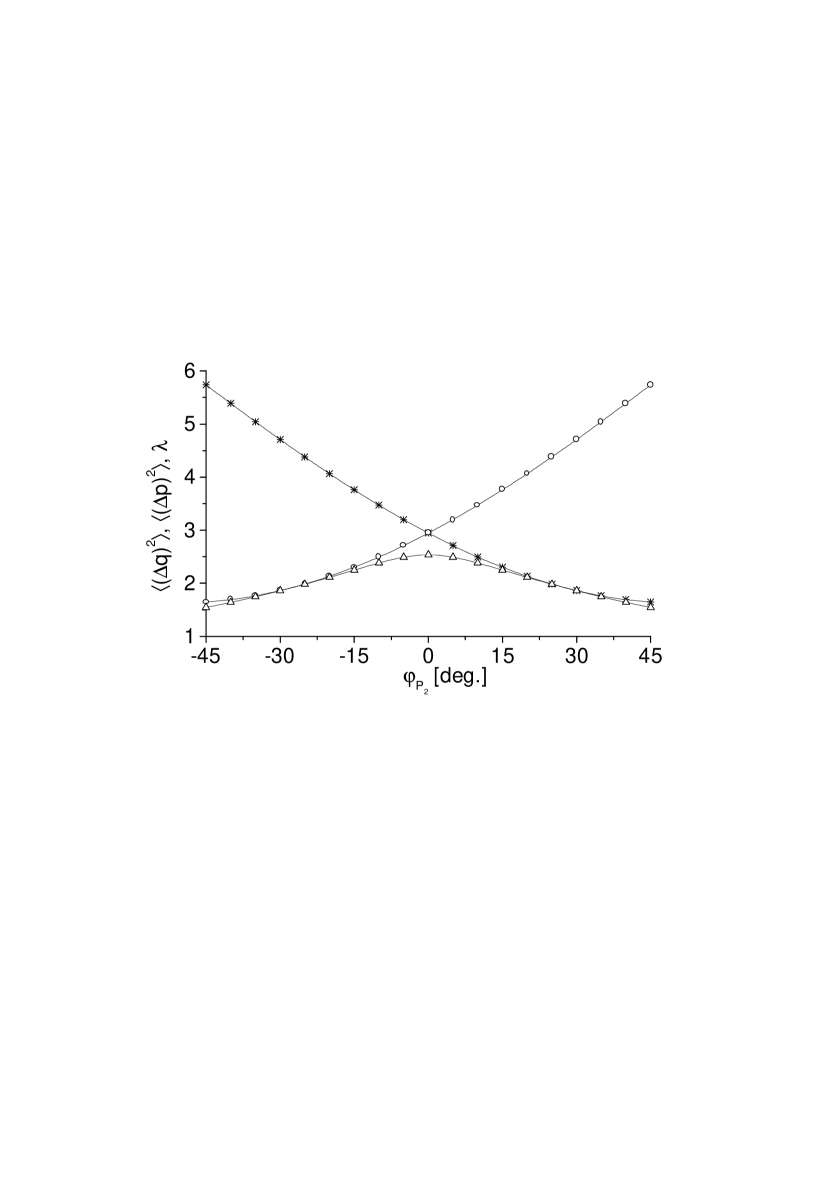
Figure 3: Demonstration of phase-controlled switching between the quadrature variances $\langle{\left[\Delta\hat{q}(L)\right]}^{2}\rangle$ $(\circ)$ and $\langle{\left[\Delta\hat{p}(L)\right]}^{2}\rangle$ $(\ast)$ (the curve denoted by $(\triangle)$ corresponds to the principal squeeze variance $\lambda(L)$) of mode $(S_{1},I_{1})$; $L=1.2$, $\Gamma_{1}=\Gamma_{2}=1$, $\kappa_{S}=\kappa_{I}=2$, $\Delta k=\Delta k_{S}=\Delta k_{I}=0$, $\xi_{P_{1}}=|\xi_{P_{2}}|=1$, $\xi_{S_{1}}=\xi_{I_{1}}=\xi_{S_{2}}=\xi_{I_{2}}=0$, $\gamma_{j}=0.2$, $\langle n_{dj}\rangle=10^{-2}$.

5.2 Linear coupling can compensate wrong phases

It is well known [14] that for small interaction lengths $z$ sub-Poissonian light can be generated in a nondegenerate down-conversion process in compound mode $(S,I)$ provided that the process is stimulated $(\xi_{S},\xi_{I}\neq 0)$ and phases of incident beams fulfil the optimum phase condition $\mbox{arg}(\xi_{S}\xi_{I}\xi_{P}^{\ast})=-\frac{\pi}{2}$. On the other hand, if either the process is spontaneous or the phase condition is strongly violated, this mode is super-Poissonian. Let us assume that the process in the first waveguide is stimulated by amplitudes $\xi_{S_{1}},\xi_{I_{1}}$ strongly violating the optimum phase condition (say $\mbox{arg}(\xi_{S_{1}}\xi_{I_{1}}\xi_{P_{1}}^{\ast})=\frac{\pi}{2}$) and the process in the second waveguide is spontaneous $(\xi_{S_{2}}=\xi_{I_{2}}=0)$. Introducing the linear coupling between the waveguides, the modes $(S_{1},I_{1})$ and $(S_{2},I_{2})$ can exhibit an interesting non-classical behaviour. The linear coupling restores the optimum phase condition and sub-Poissonian light is generated in mode $(S_{1},I_{1})$, surprisingly, for larger $z$ (see Fig. 4 (a)). Further, sub-Poissonian light is also generated in mode $(S_{2},I_{2})$ for small $z$ (Figures 4 (b) and 5), a phenomenon, which cannot be explained as easy as in the previous case. To deepen insight into this phenomenon we will resort to the analytical results. If losses are neglected, all mismatches are zero, $\kappa\equiv\kappa_{S}=\kappa_{I}$ is real, $G\equiv G_{1}=G_{2}$, and $\kappa>|G|$, we can calculate, using the results of Section 2 and (29), the correlation of fluctuations

Figure 4: The integrated intensity $\langle W(z)\rangle$ (—) and its reduced factorial moments $\frac{\langle W^{k}(z)\rangle}{{\langle W(z)\rangle}^{k}}-1$ for $k=2$ $(\ast)$, $k=3$ $(\circ)$, $k=4$ $(\triangle)$, $k=5$ $(\diamond)$ for mode $(S_{1},I_{1})$ $(a)$ and $(S_{2},I_{2})$ $(b)$; $\Gamma_{1}=\Gamma_{2}=1$, $\kappa_{S}=\kappa_{I}=5$, $\Delta k=\Delta k_{S}=\Delta k_{I}=0$, $\xi_{P_{1}}=\xi_{P_{2}}=-i$, $\xi_{S_{1}}=\xi_{I_{1}}=1$, $\xi_{S_{2}}=\xi_{I_{2}}=0$, $\gamma_{j}=0.2$, $\langle n_{dj}\rangle=10^{-2}$.

$$\langle\Delta W_{S_{2}}(z)\Delta W_{I_{2}}(z)\rangle = |G|^{2}u^{2}(z)v^{2}(z)+2\kappa^{2}|G||\xi_{S_{1}}||\xi_{I_{1}}|u(z)v^{3}(z)$$ (30)

$$\times\mbox{sin}(\varphi_{P}-\varphi_{S_{1}}-\varphi_{I_{1}}),$$

where $\varphi_{P}$, $\varphi_{S_{1}}$, $\varphi_{I_{1}}$ are the phases of input coherent amplitudes $\xi_{P}\equiv\xi_{P_{1}}=\xi_{P_{2}}$, $\xi_{S_{1}}$, $\xi_{I_{1}}$ and

$$u(z) = \mbox{cos}\left[\sqrt{2\left(\kappa^{2}-|G|^{2}\right)}z\right]-\frac{z}{4}\sqrt{2\left(\kappa^{2}-|G|^{2}\right)}\,\mbox{sin}\left[\sqrt{2\left(\kappa^{2}-|G|^{2}\right)}z\right],$$

$$v(z) = \frac{3\,\mbox{sin}\left[\sqrt{2\left(\kappa^{2}-|G|^{2}\right)}z\right]}{4\left[\sqrt{2\left(\kappa^{2}-|G|^{2}\right)}\right]}+\frac{z}{4}\,\mbox{cos}\left[\sqrt{2\left(\kappa^{2}-|G|^{2}\right)}z\right].$$ (31)

Since both the expressions on the right hand side (R.H.S.) of Eqs. (5.2) are real, only the second term on the R.H.S. of Eq. (30) can be negative depending on the sign of the product $u(z)v(z)$, and on the argument of sine function. Restricting ourselves to small $z$, we can expand $u(z)$ and $v(z)$ up to the $z^{3}$ around the origin, and approximate Eq. (30) by the expression

$$\langle\Delta W_{S_{2}}(z)\Delta W_{I_{2}}(z)\rangle\approx|G|^{2}z^{2}+2\kappa^{2}|G||\xi_{S_{1}}||\xi_{I_{1}}|z^{3}\mbox{sin}(\varphi_{P}-\varphi_{S_{1}}-\varphi_{I_{1}}).$$ (32)

Note first, that anti-correlation can only arise for sufficiently strong $\kappa$ and for sufficiently large $z$. It attains its maximum value if $\varphi_{P}-\varphi_{S_{1}}-\varphi_{I_{1}}=\mbox{arg}(\xi_{P}\xi_{S_{1}}^{\ast}\xi_{I_{1}}^{\ast})=-\frac{\pi}{2}$ (see Fig 4 (b)). It is also evident from the second term of the R.H.S. of Eq. (32) that the linear interaction enables us to affect the anti-correlation in mode $(S_{2},I_{2})$ via amplitudes $\xi_{S_{1}}$, $\xi_{I_{1}}$.

Repeating the arguments leading to the formula (30) for mode $(S_{1},I_{1})$, we obtain

$$\langle\Delta W_{S_{1}}(z)\Delta W_{I_{1}}(z)\rangle = |G|^{2}\left[2\left(|\xi_{S_{1}}|^{2}+|\xi_{I_{1}}|^{2}\right)+1\right]u^{2}(z)v^{2}(z)$$ (33)

$$-2|G||\xi_{S_{1}}||\xi_{I_{1}}|\,\mbox{sin}(\varphi_{P}-\varphi_{S_{1}}-\varphi_{I_{1}})$$

$$\times u(z)v(z)\left[u^{2}(z)+|G|^{2}v^{2}(z)\right].$$

Employing once more the expansion of (5.2) around $z=0$, we can see, that the second term on the R.H.S. of Eq. (33) is proportional to $z$ and thus its sign is given only by the argument of sine function. Our choice of the initial phases then implies that the contribution of the second term is positive in this approximation. However, the product $u(z)v(z)$ alternates and its amplitude increases with increasing $z$, suppressing the quantum noise represented by the first term on the R.H.S. of Eq. (33) and attaining the sub-Poissonian photon statistics for larger $z$.

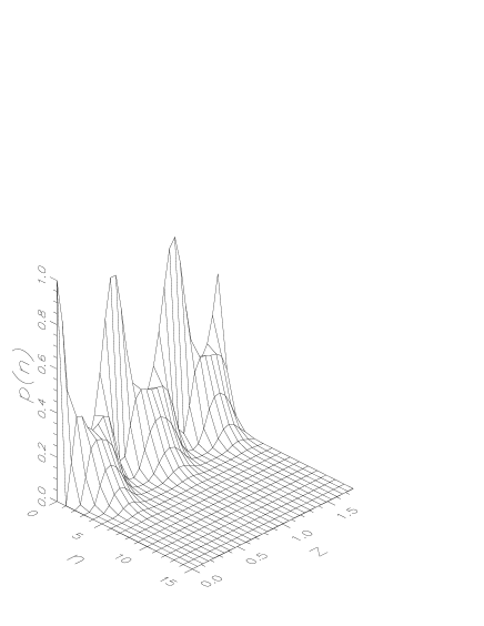
Figure 5: The sum photon number distribution $p(n,z)$ for mode $(S_{2},I_{2})$; the parameters of the process are the same as in Fig. 4.

5.3 Cross mode

Up to now we have separately discussed modes localized either in the first or in the second waveguide. This subsection will be devoted to the investigation of non-classical behaviour occuring in cross mode $(S_{1},I_{2})$.

Figure 6: (a) The quadrature variances $\langle{\left[\Delta\hat{q}(z)\right]}^{2}\rangle$ $(\circ)$, $\langle{\left[\Delta\hat{p}(z)\right]}^{2}\rangle$ $(\ast)$ and principal squeeze variance $\lambda(z)$ $(\triangle)$ for mode $(S_{1},I_{2})$, (b) integrated intensity $\langle W(z)\rangle$ (—) and its reduced factorial moments $\frac{\langle W^{k}(z)\rangle}{{\langle W(z)\rangle}^{k}}-1$ for $k=2$ $(\ast)$, $k=3$ $(\circ)$, $k=4$ $(\triangle)$, $k=5$ $(\diamond)$ for mode $(S_{1},I_{2})$; $\Gamma_{1}=\Gamma_{2}=1$, $\kappa_{S}=\kappa_{I}=4$, $\Delta k=\Delta k_{S}=\Delta k_{I}=0$, $\xi_{P_{1}}=\xi_{P_{2}}=i$, $\xi_{S_{1}}=\xi_{I_{1}}=1$, $\xi_{S_{2}}=\xi_{I_{2}}=0$, $\gamma_{j}=0.2$, $\langle n_{dj}\rangle=10^{-2}$.

The investigation of the down-conversion with strong pumping led to the conclusion that signal mode $S$ and idler mode $I$ do not exhibit any non-classical behaviour irrespectively of the fact, if they are spontaneous or stimulated by the coherent light [14]. Obviously, mode $(S_{1},I_{2})$ compounded of modes $S_{1}$ and $I_{2}$ originating from two independent down-conversion processes cannot provide a non-classical light either. However, introducing the linear interaction between the processes, we can observe squeezing of vacuum fluctuations and sub-Poissonian photon statistics simultaneously in this mode (see Figure 6). To discover the origin of these phenomena we will employ once more the analytical solution. In the spirit of the derivation of Eq. (30) we can calculate the cross-correlation function

$$D_{S_{1}I_{2}}(z)=-\kappa|G|v^{2}(z),$$ (34)

indicating, that linear exchange introduces the correlation between modes $S_{1}$ and $I_{2}$. This correlation reduces both vacuum fluctuations (see (25)) and fluctuations of photon number. To make the latter more clear, we can derive the following cross-correlation function up to $z^{3}$

$$\langle\Delta W_{S_{1}}(z)\Delta W_{I_{2}}(z)\rangle\approx-2\kappa^{2}|G||\xi_{S_{1}}||\xi_{I_{1}}|z^{3}\mbox{sin}(\varphi_{P}-\varphi_{S_{1}}-\varphi_{I_{1}}).$$ (35)

It is worth noting that the effect of noise reduction can be enhanced by increasing the amplitudes $\xi_{S_{1}}$ and $\xi_{I_{1}}$.

5.4 Mismatch-controlled switching

Before discussing the last phenomenon we would like to mention several general remarks concerning the all-optical switching. This will enlight the motivation of the following discussion. Recent theoretical investigation of couplers has led to an interesting conclusion. Not only can they serve as a passive optical switchers, but they also provide the active control of the output of a particular waveguide by means of the input of the other one. There are at least two ways how to actively control the output beams. First, the coupling lenght of the coupler can be adjusted by changing the intensity of the strong classical input field [4, 8]. Second, the phase-controlled distribution of the quantum noise in couplers can be realized [15] (see also Subection 5.1). There is, however, one more possibility how to affect the properties of the outgoing beams. Inspection of Fig. 2 reveals that one can change the dynamical behaviour of the beams by means of the global mismatch $\Delta k$. Moreover, due to its global character (it contains all wavevectors), we can control one mode by means of another one, even though they directly do not interact. The following arrangement can illustrate this. Let us assume that both processes are spontaneous, nonzero wavevectors $k_{S_{1}}$, $k_{S_{2}}$, $k_{I_{1}}$, $k_{I_{2}}$ and $k_{P_{1}}$ are chosen in such a way, that they satisfy the matching conditions $(\Delta k_{S}=\Delta k_{I}=\Delta l_{1}=0)$ and linear interaction is in operation. Now the increase of the $z$-th component $k_{P_{2}}$ of the wavevector of mode $P_{2}$ entails the inhibition of the decay of the pump photons in the first waveguide (see Figure 7). This phenomenon is easy to explain based on Fig. 2. Initially, the parameters of the coupler are such that the down-convertion part of the evolution is dominant (we are inside the hatched area). The global mismatch $\Delta k$ decreases with increasing $k_{P_{2}}$ and the linear part of evolution grows dominant. Interpreting once again the linear interaction as a sort of continuous measurement, this effect can be looked at as a complementary effect to the Zeno or anti-Zeno-like effects described in Sec. 3. Unlike in Sec. 3 where initial condition (the value of $\Delta k$) was kept constant and the strength of “measurement” was changed, here the strength of the “measurement” is the fixed quantity and the initial condition is continuously varied. In this way the influence of the “measurement” results in the speeding up the down-conversion for small values $k_{P_{2}}$ and slowing down the down-conversion for larger $k_{P_{2}}$. This corresponds to a transition from the anti-Zeno to Zeno regime.

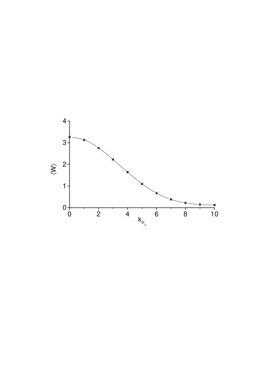
Figure 7: The dependence of the integrated intensity $\langle W(z)\rangle$ of $(S_{1},I_{1})$ (—) and $(S_{2},I_{2})$ $(\ast)$ modes on the wavevector along the $z$-axis of propagation $k_{P_{2}}$ of pump mode $P_{2}$; $L=1.5$, $\Gamma_{1}=\Gamma_{2}=1$, $\kappa_{S}=\kappa_{I}=2.5$, $k_{S_{1}}=k_{S_{2}}=6$, $k_{I_{1}}=k_{I_{2}}=4$, $k_{P_{1}}=10$, $\xi_{P_{1}}=\xi_{P_{2}}=1$, $\xi_{S_{1}}=\xi_{I_{1}}=\xi_{S_{2}}=\xi_{I_{2}}=0$, $\gamma_{j}=0.2$, $\langle n_{dj}\rangle=10^{-2}$.

It is also worth noting, that the integrated intensity of mode $(S_{2},I_{2})$ depends on $k_{P_{2}}$ in the same way as mode $(S_{1},I_{1})$ does (see Fig. 7). This can be understood as follows. At the beginning (when $k_{P_{2}}=0$) the process in the first waveguide is perfectly matched $(\Delta l_{1}=0)$ and the process in the second waveguide is strongly mismatched $(\Delta l_{2}\not=0)$. The linear interaction, however, symmetrizes the device in the way that it partially mismatches the first process and partially compensates the mismatch in the second waveguide at the same time.

6 Conclusion

The quantum dynamics and statistics of the symmetric nonlinear coupler operating by down-conversion process have been investigated. In a framework of strong pumping approximation we have solved analytically the Heisenberg-Langevin equations. The manifestation of Zeno and anti-Zeno effects has been demonstrated based on the analytical solution. The non-classical behaviour of beams involved has been studied based on numerical calculations. The phase-controlled redistribution of quantum noise between the quadratures can be achieved in mode $(S_{1},I_{1})$. The possibility of generation of sub-Poissonian light in modes $(S_{1},I_{1})$ and $(S_{2},I_{2})$ caused by the linear interaction of two super-Poissonian lights has been shown. Light exhibiting simultaneous squeezing of vacuum fluctuations and sub-Poissonian photon statistics can be obtained in cross mode $(S_{1},I_{2})$. The inhibition of the decay process in the first waveguide owing to the nonlinear matching of the second process has been observed. All these phenomena were shown to be robust against the presence of weak damping.

Appendix A Matrices $\bf b$, $\bf c$, $\bf d$ of Eq. (16)

$${\bf b}=\left[\begin{array}[]{cccc}K_{I_{1}}+K_{S_{2}}+K_{I_{2}}&i\kappa_{S}^{\ast}&iG_{1}&0\\ i\kappa_{S}&K_{S_{1}}+K_{I_{1}}+K_{I_{2}}&0&iG_{2}\\ -iG_{1}^{\ast}&0&K_{S_{1}}+K_{S_{2}}+K_{I_{2}}&-i\kappa_{I}\\ 0&-iG_{2}^{\ast}&-i\kappa_{I}^{\ast}&K_{S_{1}}+K_{S_{2}}+K_{I_{1}}\end{array}\right],\\$$

$${\bf c}=\left[\begin{array}[]{ccc}K_{I_{1}}K_{S_{2}}+L_{I}+\bar{L}_{2}&i{\kappa_{S}^{\ast}}(K_{I_{1}}+K_{I_{2}})&iG_{1}(K_{S_{2}}+K_{I_{2}})\\ i{\kappa_{S}}(K_{I_{1}}+K_{I_{2}})&K_{S_{1}}K_{I_{2}}+L_{I}+\bar{L}_{1}&{\kappa_{I}^{\ast}}G_{2}-{\kappa_{S}}G_{1}\\ -iG_{1}^{\ast}(K_{S_{2}}+K_{I_{2}})&{\kappa_{S}^{\ast}}G_{1}^{\ast}-{\kappa_{I}}G_{2}^{\ast}&K_{S_{1}}K_{I_{2}}+L_{S}+\bar{L}_{2}\\ {\kappa_{S}}G_{2}^{\ast}-{\kappa_{I}^{\ast}}G_{1}^{\ast}&-iG_{2}^{\ast}(K_{S_{1}}+K_{I_{1}})&-i\kappa_{I}^{\ast}(K_{S_{1}}+K_{S_{2}})\\ \end{array}\right.$$

$$\left.\begin{array}[]{c}{\kappa_{I}}G_{1}-{\kappa_{S}^{\ast}}G_{2}\\ iG_{2}(K_{S_{1}}+K_{I_{1}})\\ -i\kappa_{I}(K_{S_{1}}+K_{S_{2}})\\ K_{I_{1}}K_{S_{2}}+L_{S}+\bar{L}_{1}\\ \end{array}\right],$$

$${\bf d}=\left[\begin{array}[]{ccc}{\bar{L}_{2}}K_{I_{1}}+|\kappa_{I}|^{2}K_{S_{2}}&i\kappa_{S}^{\ast}L_{I}-i\kappa_{I}G_{1}G_{2}^{\ast}&iG_{1}{\bar{L}_{2}}+i{\kappa_{S}^{\ast}}{\kappa_{I}^{\ast}}G_{2}\\ i{\kappa_{S}}L_{I}-i\kappa_{I}^{\ast}G_{1}^{\ast}G_{2}&{\bar{L}_{1}}K_{I_{2}}+|\kappa_{I}|^{2}K_{S_{1}}&{\kappa_{I}^{\ast}}G_{2}K_{S_{1}}-{\kappa_{S}}G_{1}K_{I_{2}}\\ -iG_{1}^{\ast}{\bar{L}_{2}}-i\kappa_{S}\kappa_{I}G_{2}^{\ast}&{\kappa_{S}^{\ast}}G_{1}^{\ast}K_{I_{2}}-{\kappa_{I}}G_{2}^{\ast}K_{S_{1}}&{\bar{L}_{2}}K_{S_{1}}+|\kappa_{S}|^{2}K_{I_{2}}\\ \kappa_{S}G_{2}^{\ast}K_{I_{1}}-{\kappa_{I}^{\ast}}G_{1}^{\ast}K_{S_{2}}&-i{G_{2}^{\ast}}{\bar{L}_{1}}-i{\kappa_{S}^{\ast}}{\kappa_{I}^{\ast}}G_{1}^{\ast}&-i\kappa_{I}^{\ast}L_{S}+i\kappa_{S}G_{1}G_{2}^{\ast}\\ \end{array}\right.$$

$$\left.\begin{array}[]{c}-{\kappa_{S}^{\ast}}G_{2}K_{I_{1}}+{\kappa_{I}}G_{1}K_{S_{2}}\\ iG_{2}{\bar{L}_{1}}+i{\kappa_{S}}{\kappa_{I}}G_{1}\\ -i\kappa_{I}L_{S}+i{\kappa_{S}^{\ast}}G_{1}^{\ast}G_{2}\\ {\bar{L}_{1}}K_{S_{2}}+|\kappa_{S}|^{2}K_{I_{1}}\end{array}\right].$$

Appendix B Noise functions

$$B_{S_{1}}(z) = \langle\Delta\hat{A}_{S_{1}}^{\dagger}(z)\Delta\hat{A}_{S_{1}}(z)\rangle=\sum_{j=1}^{4}\left(|X_{1j}|^{2}B_{j}+2\gamma_{j}\langle{n_{dj}}\rangle\chi_{1j}\right)$$

$$+\sum_{j=1}^{2}\left(2\gamma_{j+2}\chi_{1j+2}-|X_{1j}|^{2}\right),$$

$$C_{S_{1}}(z) = \langle(\Delta\hat{A}_{S_{1}}(z))^{2}\rangle=\sum_{j=1}^{2}\left(X_{1j}^{2}C_{j}+X_{1j+2}^{2}C_{j+2}^{\ast}\right)\mbox{exp}(-2i\Delta K_{S_{1}}z),$$

$$D_{S_{1}S_{2}}(z) = \langle\Delta\hat{A}_{S_{1}}(z)\Delta\hat{A}_{S_{2}}(z)\rangle=\sum_{j=1}^{2}\left(X_{1j}X_{2j}C_{j}+X_{1j+2}X_{2j+2}C_{j+2}^{\ast}\right)$$

$$\times\mbox{exp}(-i\Delta k),$$

$$D_{S_{1}I_{1}}(z) = \langle\Delta\hat{A}_{S_{1}}(z)\Delta\hat{A}_{I_{1}}(z)\rangle=\left[\sum_{j=1}^{4}\left(X_{1j}X_{3j}^{\ast}B_{j}+2\gamma_{j}\langle{n_{dj}}\rangle\chi_{jj}^{13}\right)\right.$$

$$\left.+\sum_{j=1}^{2}\left(2\gamma_{j}\chi_{jj}^{13}-X_{1j+2}X_{3j+2}^{\ast}\right)\right]\mbox{exp}[-i(\Delta K_{S_{1}}+\Delta K_{I_{1}})z],$$

$$D_{S_{1}I_{2}}(z) = \langle\Delta\hat{A}_{S_{1}}(z)\Delta\hat{A}_{I_{2}}(z)\rangle=\left[\sum_{j=1}^{4}\left(X_{1j}X_{4j}^{\ast}B_{j}+2\gamma_{j}\langle{n_{dj}}\rangle\chi_{jj}^{14}\right)\right.$$

$$\left.+\sum_{j=1}^{2}\left(2\gamma_{j}\chi_{jj}^{14}-X_{1j+2}X_{4j+2}^{\ast}\right)\right]\mbox{exp}[-i(\Delta K_{S_{1}}+\Delta K_{I_{2}})z],$$

$$\bar{D}_{S_{1}S_{2}}(z) = -\langle\Delta\hat{A}_{S_{1}}^{\dagger}(z)\Delta\hat{A}_{S_{2}}(z)\rangle=-\left[\sum_{j=1}^{4}\left(X_{1j}^{\ast}X_{2j}B_{j}+2\gamma_{j}\langle{n_{dj}}\rangle\chi_{jj}^{21}\right)\right.$$

$$\left.+\sum_{j=1}^{2}\left(2\gamma_{j+2}\chi_{j+2j+2}^{21}-X_{1j}^{\ast}X_{2j}\right)\right]\mbox{exp}(-i\Delta k_{S}z),$$

$$\bar{D}_{S_{1}I_{1}}(z) = -\langle\Delta\hat{A}_{S_{1}}^{\dagger}(z)\Delta\hat{A}_{I_{1}}(z)\rangle=-\sum_{j=1}^{2}\left(X_{1j}^{\ast}X_{3j}^{\ast}C_{j}^{\ast}+X_{1j+2}^{\ast}X_{3j+2}^{\ast}C_{j+2}\right)$$

$$\times\mbox{exp}[i(\Delta K_{S_{1}}-\Delta K_{I_{1}})z],$$

$$\bar{D}_{S_{1}I_{2}}(z) = -\langle\Delta\hat{A}_{S_{1}}^{\dagger}(z)\Delta\hat{A}_{I_{2}}(z)\rangle=-\sum_{j=1}^{2}\left(X_{1j}^{\ast}X_{4j}^{\ast}C_{j}^{\ast}+X_{1j+2}^{\ast}X_{4j+2}^{\ast}C_{j+2}\right)$$ (40)

$$\times\mbox{exp}[i(\Delta K_{S_{1}}-\Delta K_{I_{2}})z],$$

where $X_{ij}=X_{ij}(z)$ are defined in Eq. (15) and

$$\chi_{ij} = \chi_{ij}(z)=\int_{0}^{z}|X_{ij}(z-z^{\prime})|^{2}dz^{\prime},$$

$$\chi_{jl}^{ik} = \chi_{jl}^{ik}(z)=\int_{0}^{z}X_{ij}(z-z^{\prime})X_{kl}^{\ast}(z-z^{\prime})dz^{\prime}.$$

The rest of the noise functions can be obtained using the symmetry of the model.
Acknowledgments
We would like to thank J. Peřina Jr. for help with numerical calculations. Support by Grant No. VS96028, Research project CEZ:J14 ”Wave and Particle Optics” of the Czech Ministry of Education and Grant No. 202/00/0142 of Czech Grant Agency is acknowledged.

References

• [1] Zou X Y, Wang L J and Mandel L 1991 Phys. Rev. Lett. 67 318
• [2] Luis A and Peřina J 1996 Phys. Rev. Lett. 76 4340
• [3] Luis A and Sánchez-Soto L L 1998 Phys. Rev. A 57 781
• [4] Assanto G, Laureti-Palma A, Sibilia C and Bertolotti M 1994 Opt. Commun. 110 599
• [5] Peřina J 1995 J. Mod. Opt. 42 1517
• [6] Peřina J and Peřina J Jr 1995 Quantum Semiclass. Opt. 7 541
• [7] Peřina J and Peřina J Jr 1996 J. Mod. Opt. 43 1951
• [8] Janszky J, Sibilia C, Bertolotti M, Adam P and Petak A 1995 Quantum Semiclass. Opt. 7 509
• [9] Herec J 1999 Acta Phys. Slov. 49 731
• [10] Řeháček J, Peřina J, Facchi P, Pascazio S and Mišta L Jr ”Quantum Zeno effect in a probed downconversion process” quant-ph/9911018
• [11] Graham R 1970 Quantum Optics edited by Kay S M and Maitland A (London: Academic Press) p.489
• [12] Meystre P and Sargent M III 1991 Elements of Quantum Optics (Berlin: Springer-Verlag)
• [13] Mišta L Jr 1999 Acta Phys. Slov. 49 737
• [14] Peřina J 1991 Quantum Statistics of Linear and Nonlinear Optical Phenomena (Dordrecht: Kluwer)
• [15] Mišta L Jr, Řeháček J and Peřina J 1998 J. Mod. Opt. 45 2269
• [16] Peřinová V and Peřina J 1981 Opt. Acta 28 (1981) 769