Parameters estimation in quantum optics

Abstract

We address several estimation problems in quantum optics by means of the maximum-likelihood principle. We consider Gaussian state estimation and the determination of the coupling parameters of quadratic Hamiltonians. Moreover, we analyze different schemes of phase-shift estimation. Finally, the absolute estimation of the quantum efficiency of both linear and avalanche photodetectors is studied. In all the considered applications, the Gaussian bound on statistical errors is attained with a few thousand data.

I Introduction

In order to gain information about a physical quantity one should, in principle, measure the corresponding quantum observable. In cases when the measurement can be directly implemented the statistics of the outcomes is governed (in ideal conditions, i.e. neglecting thermal, mechanical or other sources of classical noise) only by the intrinsic fluctuations of the observable, namely by the quantum nature of the system under investigation. In practice, however, it is most likely that the desired observable does not correspond to a feasible measurement scheme, or the physical quantity does not correspond to any observable at all. In such case one has to infer the value of the quantity of interest from the measurement of a different observable, or generally of a set of observables. In this situation, even in ideal conditions, the indirect parameter estimation gives an additional uncertainty for the estimated value, and the quantum estimation theory [1, 2] provides a general framework to optimize the inference procedure.

In the recent years, the indirect reconstruction of observables and quantum states has received much attention. Among the many reconstruction techniques, the most successful is quantum homodyne tomography [3], which, indeed, is the only method which has been experimentally implemented [4]. Quantum tomography provides the complete characterization of the state, i.e. the reconstruction of any quantity of interest by simple averages over experimental data. In many cases, however, one may be interested not in the complete characterization of the state, but only in some specific feature, like the phase or the amplitude of the field. Moreover, one can address the problem of characterizing an optical device, rather than a quantum state, like measuring the coupling constant of an active medium or the quantum efficiency of a photodetector. In all these cases, the desired parameter does not correspond to a measurable observable, and contains only a partial information about the quantum state of light involved in the process. Our goal is to link the estimation of such parameters with the results from feasible measurement schemes, as homodyne, heterodyne or direct detection, and to make the estimation procedure the most efficient.

Among all possible procedures for parameter estimation, the maximum-likelihood (ML) method is, in the sense discussed below, the most general, and widely usable in practice. The ML procedure answers to the following question: which values of the parameters are most likely to produce the results which we actually observe in the measurement ? This statement can be quantified, and the resulting procedure is the ML estimation of the parameters.

Recently, the ML principle has been applied to the reconstruction of the whole state of a generic quantum system [5, 6]. In that case the parameters of interest are the matrix elements of the density operator in a suitable representation. Bayesian and ML approaches have been also applied in neutron interferometry [7].

In this paper, we focus our attention on the determination of specific parameters which are relevant in quantum optics, and analyze their ML estimation procedure in some details.

In the next Section we briefly review the ML estimation procedure as well as the method to evaluate its precision. In Section III we consider the estimation of the parameters of a Gaussian state and of the coupling constants of a generic quadratic single-mode Hamiltonian. As we will show, the two estimation problems are closely related, and ML principle leads to a fully general solution. In Section IV we study different schemes of phase estimation, whereas in Section V the ML principle is applied to the estimation of the quantum efficiency of both linear and avalanche photodetectors. Section VI closes the paper by summarizing our results.

II Maximum-likelihood estimation

Here we briefly review the theory of the maximum-likelihood (ML) estimation of a single parameter. The generalization to several parameters is straightforward. Let $p(x|\lambda)$ the probability density of a random variable $x$, conditioned to the value of the parameter $\lambda$. The form of $p$ is known, but the true value of the parameter $\lambda$ is unknown, and will be estimated from the result of a measurement of $x$. Let $x_{1},x_{2},...,x_{N}$ be a random sample of size $N$. The joint probability density of the independent random variable $x_{1},x_{2},...,x_{N}$ (the global probability of the sample) is given by

$${\cal L}(x_{1},x_{2},...,x_{N}|\lambda)=\Pi_{k=1}^{N}\>p(x_{k}|\lambda)\;,$$ (1)

and is called the likelihood function of the given data sample (hereafter we will suppress the dependence of ${\cal L}$ on the data). The maximum-likelihood estimator $\lambda_{\sc ml}\equiv\lambda_{\sc ml}(\{x_{k}\})$ (MLE) of the parameter $\lambda$ maximizes ${\cal L}(\lambda)$ for variations of $\lambda$, namely it is given by the solution of the equations

$$\frac{\partial{\cal L}(\lambda)}{\partial\lambda}=0\;;\quad\frac{\partial^{2}{\cal L}(\lambda)}{\partial\lambda^{2}}<0\;.$$ (2)

Since the likelihood function is positive the first equation is equivalent to

$$\frac{\partial L(\lambda)}{\partial\lambda}=0\;,\;$$ (3)

where

$$L(\lambda)=\log{\cal L}(\lambda)=\sum_{k=1}^{N}\log p(x_{k}|\lambda)\;$$ (4)

is the so-called log-likelihood function. The form of the ML principle in Eq. (3) is the most often used in practice.

The importance of MLE stems from the following theorems [8, 9]

1. Maximum-likelihood estimators are consistent, i.e. they converge in probability to the true value of the parameter for increasing size of the data sample.

2. The distribution of MLEs tends to the normal distribution in the limit of large samples, and MLEs have minimum variance. For finite samples the variance is governed by the Cramér-Rao bound (see below).

There are also situations in which the MLE gives a poor estimation for a parameter. However, for the distributions considered here the ML procedure is statistically efficient.

In order to obtain a measure for the confidence interval in the determination of $\lambda_{\sc ml}$ we consider the variance

$$\sigma^{2}_{\lambda}=\int\left[\prod_{k}dx_{k}\>p(x_{k}|\lambda)\right]\left[\lambda_{\sc ml}(\{x_{k}\})-\lambda\right]^{2}\>\;.$$ (5)

Upon defining the Fisher information

$$F=\int dx\left[\frac{\partial p(x|\lambda)}{\partial\lambda}\right]^{2}\frac{1}{p(x|\lambda)}\;,$$ (6)

it is easy to prove [10] that

$$\sigma^{2}_{\lambda}\geq\frac{1}{N\>F}\;,$$ (7)

where $N$ is the number of measurements. The inequality in Eq. (7) is known as the Cramér-Rao bound [8] on the precision of ML estimation. Notice that this bound holds for any functional form of the probability distribution $p(x|\lambda)$, provided that the Fisher information exists $\forall\lambda$ and $\partial_{\lambda}p(x|\lambda)$ exists $\forall x$. When an experiment has ”good statistics” (i.e. a data sample large enough) the Cramér-Rao bound is saturated. As we will show in the following, the application of the ML principle in quantum optics generally corresponds to estimators for which the Cramér-Rao bound is attained with a relatively small number of measurements, i.e. the ML procedure provides an efficient estimation of the parameters. In Sections III and IV examples will be examined where the probability $p(x|\lambda)$ is Gaussian versus $x$ and not Gaussian versus the parameter $\lambda$, whereas in Section V an example with discrete measurement outcomes ($x=0,1$) will be also analyzed.

III Gaussian-state estimation

In this section we apply the ML method to estimate the quantum state of a single-mode radiation field that is characterized by a Gaussian Wigner function. Such kind of states represents the wide class of coherent, squeezed and thermal states. Apart from an irrelevant phase, we consider the Wigner function of the form

$$W(x,y)=\frac{2\Delta^{2}}{\pi}\exp\left\{-2\Delta^{2}\left[e^{-2r}(x-\hbox{Re}\mu)^{2}+e^{2r}(y-\hbox{Im}\mu)^{2}\right]\right\}\;,$$ (8)

and we apply the ML technique with homodyne detection to estimate the four real parameters $\Delta,r,\hbox{Re}\mu$ and $\hbox{Im}\mu$. The four parameters provide the number of thermal, squeezing and coherent-signal photons in the quantum state as follows

$$n_{th}=\frac{1}{2}\left(\frac{1}{\Delta^{2}}-1\right)\;,$$ (9)

$$n_{sq}=\sinh^{2}r\;,$$ (10)

$$n_{coh}=|\mu|^{2}\;.$$ (11)

In terms of density matrix, the state corresponding to the Wigner function in Eq. (8) writes

$$\varrho=D(\mu)\,S(r)\,\frac{1}{n_{th}+1}\left(\frac{n_{th}}{n_{th}+1}\right)^{a^{\dagger}a}\,S^{\dagger}(r)\,D^{\dagger}(\mu)\;,$$ (12)

where $S(r)=\exp[r(a^{2}-a^{{\dagger}2})/2]$ and $D(\mu)=\exp(\mu a^{\dagger}-\mu^{*}a)$ denote the squeezing and displacement operators, respectively.

The theoretical homodyne probability distribution at phase $\phi$ with respect to the local oscillator is given by the Gaussian [11]

$$p(x,\phi) = \sqrt{\frac{2\Delta^{2}}{\pi(e^{2r}\cos^{2}\phi+e^{-2r}\sin^{2}\phi)}}$$ (13)

$$\times \exp\left\{-\frac{2\Delta^{2}}{e^{2r}\cos^{2}\phi+e^{-2r}\sin^{2}\phi}\left[x-\hbox{Re}(\mu\,e^{-i\phi})\right]^{2}\right\}\;.$$ (14)

From Eqs. (4) and (14) one easily evaluates the log-likelihood function for a set of $N$ homodyne outcomes $x_{i}$ at random phase $\phi_{i}$ as follows

$$L = \sum_{i=1}^{N}\frac{1}{2}\log\frac{2\Delta^{2}}{\pi(e^{2r}\cos^{2}\phi_{i}+e^{-2r}\sin^{2}\phi_{i})}$$ (15)

$$- \frac{2\Delta^{2}}{e^{2r}\cos^{2}\phi_{i}+e^{-2r}\sin^{2}\phi_{i}}\left[x_{i}-\hbox{Re}(\mu\,e^{-i\phi_{i}})\right]^{2}\;.$$ (16)

The ML estimators $\Delta_{\sc ml},r_{\sc ml},\hbox{Re}\mu_{\sc ml}$ and $\hbox{Im}\mu_{\sc ml}$ are found upon maximizing Eq. (16) versus $\Delta,r,\hbox{Re}\mu$ and $\hbox{Im}\mu$.

In order to obtain a global estimation of the goodness of the state reconstruction, we evaluated the normalized overlap $\cal O$ between the theoretical and the estimated state

$${\cal O}=\frac{\hbox{Tr}[\varrho\,\varrho_{\sc ml}]}{\sqrt{\hbox{Tr}[\varrho^{2}]\,\hbox{Tr}[\varrho_{\sc ml}^{2}]}}\;.$$ (17)

Notice that ${\cal O}=1$ iff $\varrho=\varrho_{\sc ml}$. Through some Monte-Carlo simulations, we always found a value around unity, typically with statistical fluctuations over the third digit, for number of data samples $N=50000$, quantum efficiency at homodyne detectors $\eta=80\%$, and state parameters with the following ranges: $n_{th}<3$, $n_{coh}<5$, and $n_{sq}<3$. Also with such a small number of data samples, the quality of the state reconstruction is so good that other physical quantities that are theoretically evaluated from the experimental values of $\Delta_{\sc ml},r_{\sc ml},\hbox{Re}\mu_{\sc ml}$ and $\hbox{Im}\mu_{\sc ml}$ are inferred very precisely. For example, we evaluated the photon number probability of a squeezed thermal state, which is given by the integral

$$\langle n|\varrho|n\rangle=\int_{0}^{2\pi}\frac{d\phi}{2\pi}\frac{[C(\phi,n_{th},r)-1]^{n}}{C(\phi,n_{th},r)^{n+1}}\;,$$ (18)

with $C(\phi,n_{th},r)=(n_{th}+\frac{1}{2})(e^{-2r}\sin^{2}\phi+e^{2r}\cos^{2}\phi)+\frac{1}{2}$. The comparison of the theoretical and the experimental results for a state with $n_{th}=0.1$ and $n_{sq}=3$ is reported in Fig. 1. The statistical error of the reconstructed number probability affects the third decimal digit, and is not visible on the scale of the plot.

The estimation of parameters of Gaussian Wigner functions through the ML method allows one to estimate the parameters in quadratic Hamiltonians of the generic form

$$H=\alpha a+\alpha^{*}a^{\dagger}+\varphi a^{\dagger}a+\frac{1}{2}\xi a^{2}+\frac{1}{2}\xi^{*}a^{{\dagger}2}\;.$$ (19)

In fact, the unitary evolution operator $U=e^{-iHt}$ preserves the Gaussian form of an input state with Gaussian Wigner function. In other words, one can use a Gaussian state to probe and characterize an optical device described by a Hamiltonian as in Eq. (19). Assuming $t=1$ without loss of generality, the Heisenberg evolution of the radiation mode $a$ is given by

$$U^{\dagger}\,a\,U=\gamma a+\delta a^{\dagger}+\mu\;,$$ (20)

with

$$\gamma=\cos(\sqrt{\varphi^{2}-|\xi|^{2}})-i\frac{\varphi}{\sqrt{\varphi^{2}-|\xi|^{2}}}\sin(\sqrt{\varphi^{2}-|\xi|^{2}})\;,$$ (21)

$$\delta=-i\frac{\xi^{*}}{\sqrt{\varphi^{2}-|\xi|^{2}}}\sin(\sqrt{\varphi^{2}-|\xi|^{2}})\;,$$ (22)

$$\mu=\frac{\varphi\alpha^{*}-\xi^{*}\alpha}{\varphi^{2}-|\xi|^{2}}(\cos(\sqrt{\varphi^{2}-|\xi|^{2}})-1)-i\frac{\alpha^{*}}{\sqrt{\varphi^{2}-|\xi|^{2}}}\sin(\sqrt{\varphi^{2}-|\xi|^{2}})\;.$$ (23)

For an input state $\varrho$ with known Wigner function $W_{\varrho}(\beta\,,\beta^{*})$, the corresponding output Wigner function writes

$$W_{U\varrho U^{\dagger}}(\beta\,,\beta^{*})=W_{\varrho}[(\beta-\mu)\gamma^{*}-(\beta^{*}-\mu^{*})\delta\,,(\beta^{*}-\mu^{*})\gamma-(\beta-\mu)\delta^{*}]\;.$$ (24)

Hence, by estimating the parameters $\gamma,\delta,\mu$ and inverting Eqs. (23), one obtains the ML values for $\alpha,\varphi$, and $\xi$ of the Hamiltonian in Eq. (19). The present example can be used in practical applications for the estimation of the gain of a phase-sensitive amplifier or equivalently to estimate a squeezing parameter.

IV Phase estimation

The quantum-mechanical measurement of the phase of the radiation field is the essential problem of high sensitive interferometry, and has received much attention in quantum optics [12]. The problem arises because for a single mode of the electromagnetic field there is no selfadjoint operator for the phase, hence a more general description of the phase measurement is needed on the ground of estimation theory [1, 2].

In the following we apply the ML method to different schemes of phase estimation and evaluate the corresponding sensitivity.

A Heterodyne detection on coherent state

For a coherent state with amplitude $A\,e^{i\psi}$ the probability density for complex outcome $\alpha_{i}$ at the $i$-th heterodyne measurement is given by

$$p(\alpha_{i})=\frac{1}{\pi}\exp(-|\alpha_{i}-A\,e^{i\psi}|^{2})\;.$$ (25)

The max-likelihood condition $\partial L/\partial\psi=0$ provides the MLE for the phase $\psi$. One obtains $\psi_{\sc ml}=\arg(\overline{\alpha})$, where the overline denotes the experimental average over N heterodyne outcomes, namely $\overline{\alpha}=(\sum_{i=1}^{N}\alpha_{i})/N$. For small phase-shift $\psi\simeq 0$ the Cramér-Rao bound gives the constraint $\sigma_{\psi}\geq 1/\sqrt{2nN}$, $n$ being the average photon number ($n=A^{2}$).

B Homodyne detection at random phase on coherent state

In this case the homodyne probability for outcome $x_{i}$ at the $i$-th measurement at phase $\phi_{i}$ writes

$$p(x_{i},\phi_{i})=\sqrt{\frac{2}{\pi}}\exp\left\{-2[x_{i}-A\cos(\phi_{i}-\psi)]^{2}\right\}\;.$$ (26)

The ML condition provides for the estimator of $\psi$ the solution

$$\psi_{\sc ml}=\hbox{arctg}\left(\overline{x\sin\phi}/\overline{x\cos\phi}\right)\;.$$ (27)

Also in this kind of phase-detection strategy, the variance of the estimator for small phase-shift satisfies

$$\sigma_{\psi}^{2}\geq\frac{1}{2nN}\;.$$ (28)

C Homodyne detection at fixed phase on squeezed states

The use of squeezed states and homodyne detection at the phase corresponding to the squeezed quadrature offer a better result in terms of sensitivity. Consider the problem of estimating the phase $\psi$ in the state $D(A\,e^{i\psi})S(r)|0\rangle$ with $A,r>0$. The homodyne probability of outcome $y_{i}$ for the measurement of the quadrature $Y=(a-a^{\dagger})/2i$ writes

$$p(y_{i})=\sqrt{\frac{2\,e^{2r}}{\pi}}\exp\left[-2\,e^{2r}\,(y_{i}-A\sin\psi)^{2}\right]\;.$$ (29)

The MLE for $\psi$ is then given by $\psi_{\sc ml}=\hbox{arcsin}(\overline{y}/A)$. For small phase shift $\psi\simeq 0$ the Cramér-Rao bound provides the relation

$$\sigma^{2}_{\psi}\geq\frac{1}{4N\,A^{2}\,e^{2r}}.\;$$ (30)

Upon maximizing the product $A^{2}\,e^{2r}$ versus the total number of photons in the state $n=A^{2}+\sinh^{2}r$, one obtains the optimal squeezing

$$e^{2r}=2A^{2}\left[1+\sqrt{1+\frac{1}{4A^{4}}}\right]\;.$$ (31)

Notice that for $A\gg 1$, Eq. (31) requires that an equal number of squeezing and coherent photons contributes to the total average power in the radiation, namely $n_{coh}\simeq n_{sq}\simeq n/2$. In this case Eq. (30) rewrites

$$\sigma^{2}_{\psi}\geq\frac{1}{4N\,n^{2}}\;,$$ (32)

namely one obtains the ideal limit for the sensitivity of phase estimation [1, 2]. The bounds on sensitivity obtained in the previous examples are saturated within a rather small number of data samples. In Fig. 2 we compare the experimental error obtained by a Monte-Carlo simulation of homodyne detection on squeezed states using 5000 data samples with the theoretical bound of Eq. (30). We fixed the total number of photons at the value $n=50$, and varied the squeezing fraction $n_{sq}/n$. Notice how experimental and theoretical data compare very well. We estimated the statistical errors in Figs. 2-4 from the raw data by propagation of the errors on the evaluation of $\overline{y}$, namely

$$\sigma_{\psi}^{2}=\left(\frac{\partial\psi_{\sc ml}}{\partial\overline{y}}\right)^{2}\,\sigma^{2}_{\overline{y}}\;.$$ (33)

Notice that for large data samples, $\sigma_{\overline{y}}\rightarrow e^{-2r}/4N$, and one recovers Eq. (30). As shown in Figs. 2-4, our estimation of errors approaches the Cramér-Rao bound, hence proving that the ML method for the phase estimation is statistically efficient. At the optimal value of squeezing fraction [see Eq. (31)], the behavior $\sigma_{\psi}\propto 1/n$ is well reproduced, also at the small number 5000 of data samples, as shown in Fig. 3.

Unfortunately, the result in Eq. (32) is very sensible to the effect of less-than-unity quantum efficiency $\eta$ of realistic homodyne detectors. For $\eta<1$, the homodyne probability is given by a convolution of the ideal distribution in Eq. (29) with a Gaussian with variance $(1-\eta)/4\eta$. In such case, Eq. (30) is replaced by

$$\sigma^{2}_{\psi}\geq\frac{e^{-2r}+\frac{1-\eta}{\eta}}{4N\,A^{2}}\;.$$ (34)

The optimal value of the squeezing factor $e^{-2r}$ to minimize Eq. (34) at fixed total number of photons is given by the solution in the interval $I=[0,1]$ of the cubic equation

$$x^{3}+\left(4A^{2}+\frac{1-\eta}{\eta}\right)x^{2}-x-\frac{1-\eta}{\eta}=0\;.$$ (35)

Compare Fig. 2 with Fig. 4, where quantum efficiency $\eta=0.8$ has been used. Indeed, the optimal squeezing fraction rapidly approaches zero as $r\simeq A^{2}\,\eta$ for $\eta\rightarrow 0$. Such a detrimental effect of quantum efficiency is similar to the effect of losses in squeezed-state homodyne communication channels [13]. However, it can be partially stemmed by adopting a feedback-assisted homodyne detection [14].

V Absolute estimation of the quantum efficiency

In principle, in a photodetector each photon ionizes a single atom, and the resulting charge is amplified to produce a measurable pulse. In practice, however, available photodetectors are usually characterized by a quantum efficiency lower than unity, which means that only a fraction of the incoming photons lead to an electric pulse, and ultimately to a ”count”. If the resulting current is proportional to the incoming photon flux we have a linear photodetector. This is , for example, the case of the high flux photodetectors used in homodyne detection. On the other hand, photodetectors operating at very low intensities resort to avalanche process in order to transform a single ionization event into a recordable pulse. This implies that one cannot discriminate between a single photon or many photons as the outcomes from such detectors are either a ”click”, corresponding to any number of photons, or ”nothing” which means that no photons have been revealed. In this section we apply the ML principle to the absolute estimation of the quantum efficiency of both linear and avalanche photodetectors. We suppose to have at our disposal a known reference state and, from the results of a measurement upon such a state, we infer the value of the quantum efficiency.

Let us first study the case of linear photodetectors. As a reference state we consider a squeezed-coherent state, measured by homodyne detection. The effect of nonunit quantum efficiency $\eta$ on the probability distribution of homodyne detection is twofold. We have both a rescaling of the mean value and a broadening of the distribution. For a squeezed state $|x_{0},r\rangle=D(x_{0})S(r)|0\rangle$ with the direction of squeezing parallel to the signal phase and to the phase of the homodyne detection (without loss of generality we set this phase equal to zero and $x_{0},r>0$ ) we have [15]

$$p_{\eta}(x) = \frac{1}{\sqrt{2\pi\Delta^{2}}}\exp\left[-\frac{(x-\eta x_{0})^{2}}{2\Delta^{2}}\right]\;,$$ (36)

$$\Delta^{2} = \frac{1}{4}\left(e^{-2r}+1-\eta\right)\;.$$ (37)

The total number of photons of the state is given by $n=x_{0}^{2}+\sinh^{2}r$, whereas the squeezing fraction is defined as $\gamma=\sinh^{2}r/n$. Apart from an irrelevant constant, the log-likelihood function can be written as

$$-L(\eta)=\log\Delta^{2}+\frac{1}{\Delta^{2}}\left(\overline{x^{2}}+\eta x_{0}^{2}-2\eta x_{0}\overline{x}\right)\;.$$ (38)

The resulting MLE is thus given by

$$\eta_{\sc ml}=1+e^{-2r}+\frac{1}{x_{0}^{2}}\left\{1-\sqrt{1+64x_{0}^{2}\left[\overline{x^{2}}+(1+e^{-2r})(x_{0}-2\overline{x}+x_{0}e^{-2r})x_{0}\right]}\right\}\;.$$ (39)

A set of Monte Carlo simulated experiments confirmed that the Cramér-Rao bound is attained. The performances of the ML estimation can be compared to the ”naive” estimation based only on the measurement of the mean value, i.e. $\eta_{\sc av}=\overline{x}/x_{0}$. We expect this method to be less efficient, since the quantum efficiency not only rescales the mean value, but also spreads the variance of the homodyne distribution in Eq. (37). In Fig. 5, on the basis of a Monte Carlo simulated experiment, we compare the ML and the average-value methods in estimating the quantum efficiency through homodyne detection on a squeezed state. The advantages of ML method are apparent, especially for the estimation of low values of $\eta$. On the other hand, for small values of the squeezing fraction the two methods have similar performances, except for very low signals, whereas the ML estimation performs better.

Let us now consider avalanche photodetectors, which perform the ON/OFF measurement described by the two-value POM

$$\Pi_{\sc off}=\sum_{p=0}^{\infty}(1-\eta)^{p}\>|p\rangle\langle p|\qquad\Pi_{\sc on}={\bf I}-\Pi_{\sc off}\;,$$ (40)

where ${\bf I}$ denotes the identity operator. Indeed, for high quantum efficiency (close to unity) $\Pi_{\sc off}$ and $\Pi_{\sc on}$ approach the projection operator onto the vacuum state and its orthogonal subspace, respectively. With avalanche photodetectors we have only two possible outcomes: ”click” or ”no clicks” which we denote by ”1” and ”0” respectively. The log-likelihood function is given by

$$L(\eta)=(N-N_{c})\log P_{0}(\eta)+N_{c}\log[1-P_{0}(\eta)]\;,$$ (41)

where $P_{0}(\eta)=\hbox{Tr}[\varrho\Pi_{\sc off}]$ is the probability of having no clicks for the reference state described by the density matrix $\varrho$, $N$ is the total number of measurements, and $N_{c}$ is the number of events leading to a click. The maximum of $L(\eta)$, i.e. the MLE for the quantum efficiency, satisfies the equation

$$P_{0}(\eta_{\sc ml})=1-\frac{N_{c}}{N}\;,$$ (42)

whose solution, of course, depends on the choice of the reference state. The optimal choice would be using single-photon states as a reference. In this case, we have the trivial result $\eta_{\sc ml}=N_{c}/N$. However, single-photon state are not easy to prepare [16], and generally one would like to test $\eta$ for coherent pulses $|\alpha\rangle$. In this case, we have $P_{0}(\eta)=\exp(-|\alpha|^{2}\eta)$ and

$$\eta_{\sc ml}=-\frac{1}{|\alpha|^{2}}\log\left(1-\frac{N_{c}}{N}\right)\;.$$ (43)

The Fisher information is given by

$$F = \left(\frac{\partial P_{0}}{\partial\eta}\right)^{2}\frac{1}{P_{0}}+\left(\frac{\partial P_{1}}{\partial\eta}\right)^{2}\frac{1}{P_{1}}$$ (44)

$$= \frac{1}{P_{0}(1-P_{0})}\left(\frac{\partial P_{0}}{\partial\eta}\right)^{2}\;,$$ (45)

and therefore, for a weak coherent reference one has

$$F=\frac{\eta^{2}}{e^{\eta|\alpha|^{2}}-1}\simeq\frac{\eta}{|\alpha|^{2}}\,$$ (46)

and

$$\sigma_{\eta} \simeq \frac{|\alpha|}{\sqrt{\eta N}}\;.$$ (47)

VI Summary and conclusions

In quantum optics, there are several parameters of great interest corresponding to quantities that are not directly observable. Among these, we studied the parameters of a Gaussian state, the phase of a squeezed-coherent state, and the quantum efficiency of either linear or single-photon resolving photodetector. In this paper, we have applied the maximum-likelihood method to the determination of these parameters using feasible detection schemes. In particular, we have considered homodyne detection and on/off photodetection. In all cases here analyzed, the resulting estimators are efficient, unbiased and consistent, thus providing a statistically reliable determination of the parameters of interest. Moreover, by using the ML method only few thousand data are required for the precise determination of parameters. We stress that the ML procedure used in this paper can be applied to a broad class of estimation process, since it applies to any probability distribution $p(x|\lambda)$, as long as its functional form is known and the maximum of the likelihood function is unique. In conclusion, for the measurement of parameters pertaining to quantum states or optical devices, the ML procedure should be taken into account, in order to optimize data analysis and thus reducing the experimental efforts.

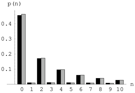
FIG. 1.: Photon-number probability of a squeezed-thermal state. The black histogram for the theoretical, the gray one reconstructed state by means of the maximum likelihood method and homodyne detection. Number of data samples $N=50000$, quantum efficiency $\eta=80\%$, number of thermal photons $n_{th}=0.1$, number of squeezing photons $n_{sq}=3$. The statistical error affects the third decimal digit, and it is not visible in the scale of the plot.

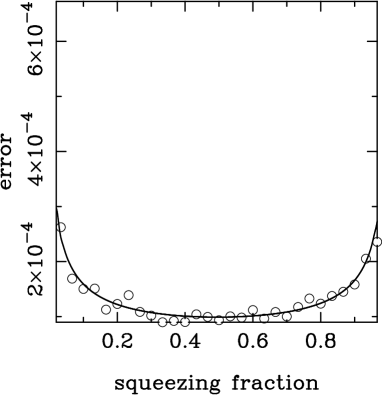
FIG. 2.: Estimation of the statistical error (circles) for the phase-shift measurement through the maximum likelihood method on a squeezed state of radiation, for different values of the degree of squeezing. The total number of photon of the state is fixed at $n=50$. The solid line represents the Cramér-Rao bound on the errors. Only 5000 homodyne data have been used, and the bound is saturated, thus proving the efficiency of the method.

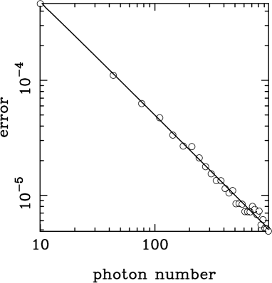
FIG. 3.: Phase sensitivity vs total number of photons achievable through homodyne detection on squeezed states and maximum likelihood estimation, with optimal fraction of squeezing photons [see Eq. (31)]. Compare the results of a Monte-Carlo simulation with 5000 homodyne outcomes (circles) with the theoretical behavior (solid line).

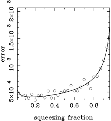
FIG. 4.: Same as in Fig. 2, but for quantum efficiency $\eta=80\%$. Notice how the best sensitivity is achieved for a smaller fraction of squeezing photons.

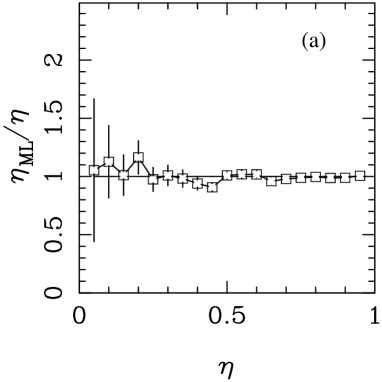
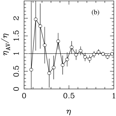
FIG. 5.: Estimation of the quantum efficiency of linear photodetectors through homodyne detection on a squeezed state. Both plots report the ratio between the estimated value of the quantum efficiency and the true value, as a function of the true value. (a) results obtained using the maximum-likelihood method; (b) results by the ”naive” average-value method. The homodyne sample consists of $50$ blocks of $50$ data each, whereas the reference state is a squeezed state with mean number of photons $n=1$ and squeezing fraction $\gamma=99\%$ (nearly a squeezed vacuum).

REFERENCES

- [1] C. W. Helstrom, Quantum Detection and Estimation Theory, Academic, New York, 1976.
- [2] A. S. Holevo. Probabilistic and statistical aspects of quantum theory, North-Holland, (Amsterdam, 1982).
- [3] For a review see: G. M. D’Ariano in Quantum Optics and Spectroscopy of Solids, ed. by A. S. Shumowsky and T. Hakiouglu (Kluwer Publishing – Amsterdam, 1997) p.175
- [4] G. Breitenbach, S. Schiller, and J. Mlynek, Nature 387 471 (1997).
- [5] K. Banaszek, Phys. Rev. A 59 4797 (1999); K. Banaszek, G. M. D’Ariano, M. G. A. Paris, and M. F. Sacchi, Phys. Rev. A 61, 10304 (2000).
- [6] Z. Hradil, J. Summhammer, and H. Rauch, Phys. Lett. A 261 20 (1999); Z. Hradil and J. Summhammer, quant-ph/9911067.
- [7] J. Rehacek et al, Phys. Rev. A. 60, 473 (1999)
- [8] H. Cramér, Mathematical methods of statistics, Princeton Press (1946).
- [9] M. Kendall and A. Stuart, The advanced theory of statistics, Griffen (1958).
- [10] H. G. Tucker, Probability and mathematical statistics, Academic Press (1962).
- [11] H. P. Yuen, Phys. Rev. A 13, 2226 (1976).
- [12] Physica Scripta T48 (1993) (special issue on Quantum Phase and Phase Dependent measurements).
- [13] G. M. D’Ariano and M. F. Sacchi, Opt. Comm. 149, 152 (1998).
- [14] G. M. D’Ariano, M. G. A. Paris, and R. Seno, Phys. Rev. A 54, 4495 (1996).
- [15] U. Leonhardt and H. Paul, Phys. Rev. A 48, 4598 (1993)
- [16] G. M. D’Ariano, L. Maccone, M. G. A. Paris, and M. F. Sacchi, Optical Fock-state synthesizer, Phys. Rev. A, in press (May 2000).