Theory of Decoherence-Free Fault-Tolerant Universal Quantum Computation

Abstract

Universal quantum computation on decoherence-free subspaces and subsystems (DFSs) is examined with particular emphasis on using only physically relevant interactions. A necessary and sufficient condition for the existence of decoherence-free (noiseless) subsystems in the Markovian regime is derived here for the first time. A stabilizer formalism for DFSs is then developed which allows for the explicit understanding of these in their dual role as quantum error correcting codes. Conditions for the existence of Hamiltonians whose induced evolution always preserves a DFS are derived within this stabilizer formalism. Two possible collective decoherence mechanisms arising from permutation symmetries of the system-bath coupling are examined within this framework. It is shown that in both cases universal quantum computation which always preserves the DFS (natural fault-tolerant computation) can be performed using only two-body interactions. This is in marked contrast to standard error correcting codes, where all known constructions using one or two-body interactions must leave the codespace during the on-time of the fault-tolerant gates. A further consequence of our universality construction is that a single exchange Hamiltonian can be used to perform universal quantum computation on an encoded space whose asymptotic coding efficiency is unity. The exchange Hamiltonian, which is naturally present in many quantum systems, is thus asymptotically universal.

I Introduction

The discovery that information encoded over quantum systems can exhibit strange and wonderful computational [1, 2] and information theoretic [3, 4] properties has led to an explosion of interest in understanding and exploiting the “quantumness” of nature. For the use of quantum information to progress beyond mere theoretical constructs into the realm of testable and useful implementations and experiments, it is essential to develop techniques for preserving quantum coherences. In particular, the coupling of a quantum system to its environment leads to a process known as decoherence, in which encoded quantum information is lost to the environment. In order to remedy this problem active quantum error correction codes (QECCs) [5, 6, 7, 8, 9] have been developed, by analogy with classical error correction. These codes encode quantum information over an entangled set of codewords, the structure of which serves to preserve the quantum information, when used in conjunction with a frequently recurring error correcting procedure. It has been shown that when the rate of decoherence is below a certain threshold, fault tolerant quantum information manipulation is possible[10, 11, 12]. Since it is believed that there are no systems for which the decoherence mechanism entirely vanishes, QECCs will be essential if quantum information manipulation is to become practical.

An alternative approach has been proposed and developed recently, in which the central motivation is the desire to reduce the effect of a specific decoherence mechanism. This is the decoherence-free subspace (DFS) approach (also referred to as “error avoiding”, or “noiseless” quantum codes) [13, 14, 15, 16, 17, 18, 19, 20, 21, 22, 23, 24, 25, 26]. In contrast to the active mode of QECC, DFS theory can be viewed as providing a passive approach, where a specific symmetry of the system-bath coupling is employed in order to seek out a quiet corner of the system’s Hilbert space which does not experience decoherence. Information encoded here over a subspace of (usually entangled) system states is robust against a specific form of decoherence. We shall refer to this as the “DFS supporting decoherence mechanism”. When this is the dominant form of decoherence in the physical system, there are major gains to be had by operating in the DFS. Previous work has shown that collective decoherence of the type experienced in condensed phase systems at low temperatures can be successfully eliminated in this way [27, 28]. Further research showed that DFSs are robust to perturbing error processes [21, 24], and are thus ideally suited for concatenation in a QECC [22].

The motivating goal behind the DFS approach is to use symmetry first. Thus, one first identifies a DFS for the major sources of decoherence, via the symmetry of the interaction with the environment. One then proceeds to use the DFS states as a basis for a QECC which can deal with additional perturbing error processes. In order for this scheme to be credible, DFSs must support the ability to perform universal quantum computation on the encoded states. Towards this end, certain existential results [29] have been derived showing that in principle universal quantum computation can be performed on any DFS. Constructive results for a set of universal quantum gates on a particular class DFSs were subsequently constructed in [23] using known QECC constructions. However, these gates were constructed in such a way that during the operation of the gate, states within a DFS are taken outside of this subspace. Thus these gates would necessarily need to operate on a timescale faster than the DFS supporting decoherence mechanism, in order to be applied efficiently to a concatenated DFS-QECC scheme. Similarly, a universal computation result on DFSs for atoms in cavities was recently presented by Beige et al. in [30, 31]. It assumes that the interaction driving a system out of the DFS is much weaker than the coupling of non DF-states to the environment. It is then possible to make use of an environment-induced quantum Zeno effect. In order to make use of the robustness condition without resorting to gates which can be made faster than the main DFS supporting decoherence mechanism, one would prefer to explicitly construct a set of Hamiltonians which can be used to perform universal quantum computation, but which never allow states in the DFS to leak out of the DFS. Imperfections in these gates may be dealt with by the concatenation technique of [22] (see also [25]).

In addition, one would, from a practical standpoint, like to use Hamiltonians which involve at most two-body interactions (under the assumption that any three-body interactions will be weak and not useful for operations which must compete with the decoherence rate). In [32] such Hamiltonians were used for the important decoherence mechanism known as “collective decoherence”, on a system of $4$ physical qubits. In collective decoherence the bath cannot distinguish between individual system qubits, and thus couples in a collective manner to the qubits. The corresponding two-body Hamiltonians used to implement universal quantum computation are those that preserve the collective symmetry: the exchange interaction between pairs of qubits. The first and main purpose of this paper is therefore to extend the constructive results obtained in [32] to other forms of collective decoherence and to larger DFSs. Two different forms of collective decoherence are considered here, and constructive results are obtained for these on DFSs of arbitrary numbers of qubits. These results have implications that extend far beyond the problem of dealing with collective decoherence. Since they imply that the exchange interaction by itself is sufficient to implement universal quantum computation on a subspace, it follows that using encoded (rather than physical) qubits can be advantageous when resources for physical operations are limited. After all, the standard results for universal quantum computation employ either arbitrary single-qubit operations in addition to a non-trivial two-qubit gate (e.g., a controlled-NOT), or at least two non-commuting two-qubit Hamiltonians [33, 34, 35, 36, 37]. These issues will be explored in a separate publication.

Previous work established that DFSs correspond to the degenerate component of a QECC [22, 38]. A second purpose of this work is to present new results on a recently discovered generalization of DFSs, which has been termed “noiseless subsystems”, and arises from a theory of QECC for general decoherence mechanisms [39, 40]. In line with our previously established terminology [21] we will refer to these as “decoherence-free subsystems”, where we take the term “decoherence” to mean both dephasing ($T_{2}$) and dissipation ($T_{1}$). Essentially, the generalization corresponds to allowing for information to be encoded into states transforming according to arbitrary-dimensional irreducible representations (irreps) of the decoherence-operators’ algebra, instead of just one-dimensional irreps as in the decoherence-free subspace case (we will present precise definitions later in this paper). These results all arise from a basic theorem on algebras that are closed under the Hermitian conjugation operation (“$\dagger$-closed algebras”), and thereby unify the role of symmetry in both decoherence-free subspaces and quantum error correction. In this paper we extend the decoherence-free subsystem concept to situations governed by essentially non-$\dagger$-closed evolution. Such situations arise from non-Hermitian terms in the system-bath interaction, which may occur, e.g., in generalized master equation and conditional Hamiltonian representations of open quantum dynamics [41]. In particular, we derive an if and only if (iff) condition for the existence of decoherence-free subsystems with dynamics governed by a semigroup master equation. This is important because it is well known in decoherence-free subspace theory that such non-$\dagger$-closed evolution can support different DFSs than in the $\dagger$-closed case. A similar result is now shown here to hold for the decoherence-free subsystems.

Existential results for universal quantum computation on decoherence-free subsystems also exist [42]. The universal quantum computation results we obtain in this paper extend beyond decoherence-free subspaces: we show how to achieve constructive universal quantum computation on the decoherence-free subsystems supported under collective decoherence. This most significant achievement of our paper settles the question of universal quantum computation under collective decoherence using realistic Hamiltonians.

Another aim of this paper is to elucidate the close link between DFS and QECC. In [22, 38] it was shown that DFSs are in fact maximally degenerate QECCs. This result was derived from the general condition for a code to be a QECC [8]. A very fruitful approach towards QECC has been the stabilizer formalism developed in [9] which led to the theory of universal fault-tolerant computation on QECCs [43]. In [23] we considered DFSs as abelian stabilizer codes. Here we generalize the stabilizer-framework to non-abelian stabilizers, and show that in general DFSs are stabilizer-codes that protect against errors in the stabilizer itself. This perspective allows in return to view QECCs as DFSs against a certain kind of errors, and establishes a kind of duality of QECCs and DFSs.

The paper is structured as follows: In Section II we review decoherence-free subsystems and place them into the context of the Markovian master equation. For decoherence-free subspaces this has been done in [21, 24]. These earlier results are therefore generalized here to subsystems. In Section III we introduce a generalized stabilizer-formalism for DFS, and connect to the theory of stabilizers on QECC developed in [9]. This allows us to treat DFS and QECC within the same framework. It also sheds some light on the duality between DFS and QECC, in particular on the performance of a DFS viewed as a QECC and vice versa. In Section IV we deal with universal computation on DFS within both the stabilizer-framework and the representation-theoretic approach. We derive fault-tolerance properties of the universal operations. In particular, we show how to obtain operations that keep the states within a DFS during the entire switching-time of a gate. Further we define the allowed compositions of operations and review results on the length of gate sequences in terms of the desired accuracy of the target gates. In Section V we introduce the model of collective decoherence. Section VI explicitly deals with the abelian case of weak collective decoherence in which system-bath interaction coupling involves only a single system operator. Stabilizer and error-correcting properties are developed for this case, and it is shown how universal computation can be achieved. The same is done for the non-abelian and more general case of strong collective decoherence in Section VII. For both weak and strong collective decoherence we show how to fault-tolerantly encode into and read out of the respective DFSs. Finally, we analyze in Section VIII how to concatenate DFSs and QECCs to make them more robust against perturbing errors (as proposed in [22]) and show how the universality results can be applied to achieve fault-tolerant universal computation on these powerful concatenated codes. We conclude in Section IX. Derivations and proofs of a more technical nature are presented in the Appendix.

II Overview of Decoherence-Free Subspaces and Subsystems

A Decoherence-Free Subspaces

Consider the dynamics of a system $S$ (the quantum computer) coupled to a bath $B$ via the Hamiltonian

$${\bf H}={\bf H}_{S}\otimes{\bf I}_{B}+{\bf I}_{S}\otimes{\bf H}_{B}+{\bf H}_{I},$$ (1)

where ${\bf H}_{S}$ (${\bf H}_{B}$) [the system (bath) Hamiltonian] acts on the system (bath) Hilbert space ${\cal H}_{S}$ (${\cal H}_{B}$), ${\bf I}_{S}$ (${\bf I}_{B}$) is the identity operator on the system (bath) Hilbert space, and ${\bf H}_{I}$, which acts on both the system and bath Hilbert spaces ${\cal H}_{S}\otimes{\cal H}_{B}$, is the interaction Hamiltonian containing all the nontrivial couplings between system and bath. In general ${\bf H}_{I}$ can be written as a sum of operators which act separately on the system (${\bf S}_{\alpha}$’s) and on the bath (${\bf B}_{\alpha}$’s):

$${\bf H}_{I}=\sum_{\alpha}{\bf S}_{\alpha}\otimes{\bf B}_{\alpha}.$$ (2)

In the absence of an interaction Hamiltonian (${\bf H}_{I}=0$), the evolution of the system and the bath are separately unitary: ${\bf U}(t)=\exp[-i{\bf H}t]=\exp[-i{\bf H}_{S}t]\otimes\exp[-i{\bf H}_{B}t]$ (we set $\hbar=1$ throughout). Information that has been encoded (mapped) into states of the system Hilbert space remains encoded in the system Hilbert space if ${\bf H}_{I}=0$. However in the case when the interaction Hamiltonian contains nontrivial couplings between the system and the bath, information that has been encoded over the system Hilbert space does not remain encoded over solely the system Hilbert space but spreads out instead into the combined system and bath Hilbert space as the time evolution proceeds. Such leakage of quantum information from the system to the bath is the origin of the decoherence process in quantum mechanics.

Let $\tilde{{\cal H}}_{S}$ be a subspace of the system Hilbert space with a basis $|\tilde{\imath}\rangle$. The evolution of such a subspace will be unitary [16, 22] if and only if (i)

$${\bf S}_{\alpha}|\tilde{\imath}\rangle=c_{\alpha}|\tilde{\imath}\rangle,\quad c_{\alpha}\in{\rm\kern 2.40005pt\vrule width=0.39993pt,height=6.28612pt,depth=-0.3014pt\kern-3.00003ptC}$$ (3)

for all $|\tilde{\imath}\rangle\in\tilde{{\cal H}}_{S}$ and for all ${\bf S}_{\alpha}$, (ii) ${\bf H}_{S}$ does not mix states within the subspace with states that are outside of the subspace ($\langle j^{\prime}|{\bf H}_{S}|\tilde{\imath}\rangle=0$ for all $|\tilde{\imath}\rangle$ in the subspace and all $|j^{\prime}\rangle$ outside of the subspace: ${\bf H}_{S}=\tilde{{\bf H}}_{S}\oplus{\bf H}_{S}^{\prime}$) and (iii) system and bath are initially decoupled ${\bf\rho}(0)={\bf\rho}_{S}(0)\otimes{\bf\rho}_{B}(0)$. We call a subspace of the system’s Hilbert space which fulfills these requirements a decoherence-free subspace (DFS).

The above formulation of DFSs in terms of a larger closed system is exact. It is extremely useful for finding DFSs, providing often the most direct route via simple examination of the system components of the interaction Hamiltonian. In practical situations, however, the closed-system formulation of DFSs is often too strict. This is because the closed-system formulation incorporates the possibility that information which is put into the bath will back-react on the system and cause a recurrence. Such interactions will always occur in the closed-system formulation (due to the the Hamiltonian being Hermitian). However, in many practical situations the likelihood of such an event is extremely small. Thus, for example, an excited atom which is in a “cold” bath will radiate a photon and decohere but the bath will not in turn excite the atom back to its excited state, except via the (extremely long) recurrence time of the emission process. In these situations a more appropriate way to describe the evolution of the system is via a quantum dynamical semigroup master equation [44, 45]. By assuming that (i) the evolution of system density matrix is a one-parameter semigroup, (ii) the system density matrix retains the properties of a density matrix including “complete positivity”, and (iii) the system and bath density matrices are initially decoupled, Lindblad [44] has shown that the most general evolution of the system density matrix ${\bf\rho}_{S}(t)$ is governed by the master equation

$${\frac{d{\bf\rho}_{S}(t)}{dt}} = -i[{\bf H}_{S},{\bf\rho}_{S}(t)]+{\tt L}_{D}[{\bf\rho}_{S}(t)]$$ (4)

$${\tt L}_{D}[{\bf\rho}_{S}(t)] = {\frac{1}{2}}\sum_{\alpha,\beta=1}^{M}a_{\alpha\beta}\left([{\bf F}_{\alpha},{\bf\rho}_{S}(t){\bf F}_{\beta}^{\dagger}]+[{\bf F}_{\alpha}{\bf\rho}_{S}(t),{\bf F}_{\beta}^{\dagger}]\right)$$ (5)

where ${\bf H}_{S}$ is the system Hamiltonian, the operators ${\bf F}_{\alpha}$ constitute a basis for the $M$-dimensional space of all bounded operators acting on ${\cal H}_{S}$, and $a_{\alpha\beta}$ are the elements of a positive semi-definite Hermitian matrix. As above, let $\tilde{{\cal H}}_{S}$ be a subspace of the system Hilbert space ${\cal H}_{S}$ with a basis $|\tilde{\imath}\rangle$. The evolution over such a subspace is then unitary [21] iff

$${\bf F}_{\alpha}|\tilde{\imath}\rangle=c_{\alpha}|\tilde{\imath}\rangle,\quad c_{\alpha}\in{\rm\kern 2.40005pt\vrule width=0.39993pt,height=6.28612pt,depth=-0.3014pt\kern-3.00003ptC}$$ (6)

for all $|\tilde{\imath}\rangle$ and for all ${\bf F}_{\alpha}$. While this condition appears to be identical to Eq (3), there is an important difference between the ${\bf S}_{\alpha}$’s and the ${\bf F}_{\alpha}$’s which makes these two decoherence-freeness conditions different. In the Hamiltonian formulation of DFSs, the Hamiltonian is Hermitian. Thus the expansion for the interaction Hamiltonian Eq. (2) can always be written such that the ${\bf S}_{\alpha}$ are also Hermitian. On the other hand, the ${\bf F}_{\alpha}$’s in the master equation, Eq. (5), need only be bounded operators acting on ${\cal H}_{S}$ and thus the ${\bf F}_{\alpha}$’s need not be Hermitian. Because of this difference, Eq. (6) allows for a broader range of subspaces than Eq. (3). For example consider the situation where there are only two nonzero terms in a master equation for a two-level system, corresponding to ${\bf F}_{1}=\sigma_{-}$ and ${\bf F}_{2}=\sigma_{z}$ where $\sigma_{-}=|0\rangle\langle 1|$ and $\sigma_{z}=|0\rangle\langle 0|-|1\rangle\langle 1|$ (e.g., cooling with phase damping). In this case there is a DFS corresponding to the single state $|0\rangle$. In the Hamiltonian formulation, inclusion of ${\bf S}_{1}=\sigma_{-}$ in the interaction Hamiltonian expansion Eq. (2) would necessitate a second term in the Hamiltonian with ${\bf S}_{2}=\sigma_{-}^{\dagger}$, along with the ${\bf S}_{z}=\sigma_{z}$ as above. For this set of operators, however, Eq. (3) allows for no DFS.

B Decoherence-Free Subsystems

If one desires to encode quantum information over a subspace and requires that this information remains decoherence-free, then Eqs. (3),(6) provide necessary and sufficient conditions for the existence of such DFSs. The notion of a subspace which remains decoherence-free throughout the evolution of a system is not, however, the most general method for providing decoherence-free encoding of information in a quantum system. Recently, Knill, Laflamme, and Viola [39] have discovered a method for decoherence-free coding into subsystems instead of into subspaces.

Decoherence-free subsystems [39, 42, 46] are most easily presented in the Hamiltonian formulation of decoherence. Let ${\cal A}$ denote the associative algebra formed by the system Hamiltonian ${\bf H}_{S}$ and the system components of the interaction Hamiltonian, the ${\bf S}_{\alpha}$’s. To simplify our discussion we will assume that the system Hamiltonian vanishes. (It is easy to incorporate the system Hamiltonian into the ${\bf S}_{\alpha}$’s when one desires that the system evolution preserves the decoherence-free subsystem.) We also assume that the identity operator is included as ${\bf S}_{0}={\bf I}_{S}$ and ${\bf B}_{0}={\bf I}_{B}$. This will have no observable consequence but allows for the use of an important representation theorem. ${\cal A}$ consists of linear combinations of products of the ${\bf S}_{\alpha}$’s. Because the Hamiltonian is Hermitian the ${\bf S}_{\alpha}$’s must be closed under Hermitian conjugation: ${\cal A}$ is a $\dagger$-closed operator algebra. A basic theorem of such operator algebras which include the identity operator states that, in general, ${\cal A}$ will be a reducible subalgebra of the full algebra of operators on ${\cal H}_{S}$ [47]. This means that the algebra is isomorphic to a direct sum of $d_{J}\times d_{J}$ complex matrix algebras, each with multiplicity $n_{J}$:

$${\cal A}\cong\bigoplus_{J\in{\cal J}}{\bf I}_{n_{J}}\otimes{\cal M}(d_{J},{\rm\kern 2.40005pt\vrule width=0.39993pt,height=6.28612pt,depth=-0.3014pt\kern-3.00003ptC}).$$ (7)

Here ${\cal J}$ is a finite set labeling the irreducible components of ${\cal A}$, and ${\cal M}(d_{J},{\rm\kern 2.40005pt\vrule width=0.39993pt,height=6.28612pt,depth=-0.3014pt\kern-3.00003ptC})$ denotes a $d_{J}\times d_{J}$ complex matrix algebra. It is also useful at this point to introduce the commutant ${\cal A}^{\prime}$ of ${\cal A}$. This is the set of operators which commutes with the algebra ${\cal A}$, ${\cal A}^{\prime}=\left\{{\bf X}:[{\bf X},{\bf A}]=0,\forall{\bf A}\in{\cal A}\right\}$. They also form a $\dagger$-closed algebra, which is reducible to

$${\cal A}^{\prime}=\bigoplus_{J\in{\cal J}}{\cal M}(n_{J},{\rm\kern 2.40005pt\vrule width=0.39993pt,height=6.28612pt,depth=-0.3014pt\kern-3.00003ptC})\otimes{\bf I}_{d_{J}}$$ (8)

over the same basis as ${\cal A}$ in Eq. (7).

The structure implied by Eq. (7) is illustrated schematically as follows, for some system operator ${\bf S}_{\alpha}$:

⋱J=|𝒥|]subscript𝐒𝛼delimited-[]fragments fragments missing-subexpressionmissing-subexpression⋱missing-subexpressionmissing-subexpressionmissing-subexpressionmissing-subexpressionfragmentsJ|J|{\bf S}_{\alpha}=\left[\begin{tabular}[]{cccc}\cline{1-1}\cr\vrule\lx@intercol\hfil$J=1$\hfil\lx@intercol &\vrule\lx@intercol\hfil\hfil\lx@intercol &&\\ \cline{1-2}\cr&\vrule\lx@intercol\hfil$J=2$\hfil\lx@intercol &\vrule\lx@intercol\hfil\hfil\lx@intercol &\\ \cline{2-2}\cr&&$\ddots$&\\ \cline{4-4}\cr&&&\vrule\lx@intercol\hfil$J=|{\cal J}|$\hfil\lx@intercol\vrule\lx@intercol \\ \cline{4-4}\cr\end{tabular}\right]

=J1=J2=J1=J2 (9)

where a typical block with given $J$ has the structure:

$$J\text{ given}\text{:\quad}\left[\begin{tabular}[]{ccccccccccc}\cline{1-3}\cr\vrule\lx@intercol\hfil\hfil\lx@intercol &&&\vrule\lx@intercol\hfil\hfil\lx@intercol &&&&&&&\\ \vrule\lx@intercol\hfil\hfil\lx@intercol &$M_{\alpha}$&&\vrule\lx@intercol\hfil\hfil\lx@intercol &&&&&&&$\lambda=0$\\ \vrule\lx@intercol\hfil\hfil\lx@intercol &&&\vrule\lx@intercol\hfil\hfil\lx@intercol &&&$\mu$&&&&\\ \cline{1-6}\cr&&&\vrule\lx@intercol\hfil\hfil\lx@intercol &&&\vrule\lx@intercol\hfil$0$\hfil\lx@intercol &&&&\\ &&&\vrule\lx@intercol\hfil\hfil\lx@intercol &$M_{\alpha}$&&\vrule\lx@intercol\hfil$\vdots$\hfil\lx@intercol &&&&$\lambda=1$\\ &&&\vrule\lx@intercol\hfil\hfil\lx@intercol &&&\vrule\lx@intercol\hfil$d_{J}-1$\hfil\lx@intercol &&&&\\ \cline{4-6}\cr&&$\mu^{\prime}:$&$0$&$\cdots$&$d_{J}-1$&$\ddots$&&&&\\ \cline{8-10}\cr&&&&&&&\vrule\lx@intercol\hfil\hfil\lx@intercol &&&\vrule\lx@intercol\hfil\hfil\lx@intercol \\ &&&&&&&\vrule\lx@intercol\hfil\hfil\lx@intercol &$M_{\alpha}$&&\vrule\lx@intercol\hfil$\lambda=n_{J}-1$\hfil\lx@intercol \\ &&&&&&&\vrule\lx@intercol\hfil\hfil\lx@intercol &&&\vrule\lx@intercol\hfil\hfil\lx@intercol \\ \cline{8-10}\cr\end{tabular}\right]$$ (10)

Associated with this decomposition of the algebra ${\cal A}$ is the decomposition over the system Hilbert space:

$${\cal H}_{S}=\sum_{J\in{\cal J}}{\rm\kern 2.40005pt\vrule width=0.39993pt,height=6.28612pt,depth=-0.3014pt\kern-3.00003ptC}^{n_{J}}\otimes{\rm\kern 2.40005pt\vrule width=0.39993pt,height=6.28612pt,depth=-0.3014pt\kern-3.00003ptC}^{d_{J}}.$$ (11)

Decoherence-free subsystems are defined as the situation in which information is encoded in a single subsystem space ${\rm\kern 2.40005pt\vrule width=0.39993pt,height=6.28612pt,depth=-0.3014pt\kern-3.00003ptC}^{n_{J}}$ of Eq. (11) (thus the dimension of the decoherence-free subsystem is $n_{J}$). The decomposition in Eq. (7) reveals that information encoded in such a subsystem will always be affected as identity on the subsystem space ${\rm\kern 2.40005pt\vrule width=0.39993pt,height=6.28612pt,depth=-0.3014pt\kern-3.00003ptC}^{n_{J}}$, and thus this information will not decohere. It should be noted that the tensor product nature which gives rise to the name subsystem in Eq. (7) is a tensor product over a direct sum, and therefore will not in general correspond to the natural tensor product of qubits. Further, it should be noted that the subsystem nature of the decoherence implies that the information should be encoded in a separable way. Over the tensor structure of Eq. (11) the density matrix should split into two valid density matrices: ${\bf\rho}_{S}(0)={\bf\rho}\otimes{\bf\gamma}$ where ${\bf\rho}$ is the decoherence-free subsystem and ${\bf\gamma}$ is the corresponding component of the density matrix which does decohere. Finally it should be pointed out that not all of the subsystems in the different irreducible representations can be simultaneously used: (phase) decoherence will occur between the different irreducible components of the Hilbert space labeled by $J\in{\cal J}$. For this reason, from now on we restrict our attention to the subspace defined by a given $J$.

Decoherence-free subspaces are now easily connected to decoherence-free subsystems. Decoherence-free subspaces correspond to decoherence-free subsystems possessing one-dimensional irreducible matrix algebras: ${\cal M}(1,{\rm\kern 2.40005pt\vrule width=0.39993pt,height=6.28612pt,depth=-0.3014pt\kern-3.00003ptC})$. The multiplicity of these one-dimensional irreducible algebras is the dimension of the decoherence-free subspaces. In fact it is easy to see how the decoherence-free subsystems arise out of a non-commuting generalization of the decoherence-free subspace conditions. Let $\{|\lambda_{\mu}\rangle\}$, $1\leq\lambda\leq n_{J}$ and $1\leq\mu\leq d_{J}$, denote a subspace of ${\cal H}_{S}$ with given $J$. Then the condition for the existence of an irreducible decomposition as in Eq. (7) is

$${\bf S}_{\alpha}|\lambda_{\mu}\rangle=\sum_{\mu^{\prime}=1}^{d_{J}}M_{\mu\mu^{\prime},\alpha}|\lambda_{\mu^{\prime}}\rangle,$$ (12)

for all ${\bf S}_{\alpha}$, $\lambda$ and $\mu$. Notice that $M_{\mu\mu^{\prime},\alpha}$ is not dependent on $\lambda$, in the same way that $c_{\alpha}$ in Eq. (3) is not the same for all $|\tilde{\imath}\rangle$ (there $\mu=1$ and fixed). Thus for a fixed $\lambda$, the subspace spanned by $|\lambda_{\mu}\rangle$ is acted upon in some nontrivial way. However, because $M_{\mu\mu^{\prime},\alpha}$ is not dependent on $\lambda$, each subspace defined by a fixed $\mu$ and running over $\lambda$ is acted upon in an identical manner by the decoherence process.

At this point it should be noted that the generalization of the Lindblad master equation Eq. (5) with a decoherence-free subspace to the corresponding master equation for a decoherence-free system is not trivial. This is because, as above, the ${\bf F}_{\alpha}$ operators in Eq. (5) are (for all practical purposes) not required to be closed under conjugation. The representation theorem Eq. (7) is hence not directly applicable. We will show, however, that the master equation analog of Eq. (12)

$${\bf F}_{\alpha}|\lambda_{\mu}\rangle=\sum_{\mu^{\prime}=1}^{d_{J}}M_{\mu\mu^{\prime},\alpha}|\lambda_{\mu^{\prime}}\rangle$$ (13)

provides a necessary and sufficient condition for the preservation of decoherence-free subsystems.

As above, we consider a subspace of the system Hilbert space spanned by $|\lambda_{\mu}\rangle$, with $1\leq\lambda\leq n_{J}$ and $1\leq\mu\leq d_{J}$. Our notation will be significantly simpler if we explicitly write out the formal tensor product over this subspace: $|\lambda_{\mu}\rangle=|\lambda\rangle\otimes|\mu\rangle$. In the subsystem notation, we claim that the decoherence-free subsystem condition is

$${\bf F}_{\alpha}|\lambda\rangle\otimes|\mu\rangle=|\lambda\rangle\otimes{\bf M}_{\alpha}|\mu\rangle.$$ (14)

A proper decomposition of the system Hilbert space requires, as noted above, that the system density matrix is a tensor product of two valid (Hermitian, positive) density matrices:

$${\bf\rho}_{S}(0)=\sum_{\lambda\lambda^{\prime},\mu\mu^{\prime}}\rho_{\lambda\lambda^{\prime}}(0)\gamma_{\mu\mu^{\prime}}(0)|\lambda_{\mu}\rangle\langle\lambda_{\mu^{\prime}}^{\prime}|={\bf\rho}(0)\otimes{\bf\gamma}(0),$$ (15)

where $\rho(0)$ contains the information which will remain decoherence-free, and $\gamma(0)$ is an arbitrary but valid density matrix.

In general the operators ${\bf F}_{\alpha}$ will not be decomposable as a single tensor product corresponding to ${\bf\rho}(0)\otimes{\bf\gamma}(0)$. Rather, they will be a sum over such tensor products, corresponding to an expansion over an operator basis: ${\bf F}_{\alpha}=\sum_{p}{\bf N}_{\alpha}^{p}\otimes{\bf M}_{\alpha}^{p}$. The decohering generator of evolution (5) thus becomes

$${\tt L}_{D}[{\bf\rho}_{S}(0)] = {\frac{1}{2}}\sum_{\alpha\beta}a_{\alpha\beta}\sum_{pq}\left(2{\bf N}_{\alpha}^{p}{\bf\rho}(0){\bf N}_{\beta}^{q\dagger}\otimes{\bf M}_{\alpha}^{p}{\bf\gamma}(0){\bf M}_{\beta}^{q\dagger}-{\bf N}_{\beta}^{q\dagger}{\bf N}_{\alpha}^{p}{\bf\rho}(0)\otimes{\bf M}_{\beta}^{q\dagger}{\bf M}_{\alpha}^{p}{\bf\gamma}(0)\right.$$ (16)

$$- \left.{\bf\rho}(0){\bf N}_{\beta}^{q\dagger}{\bf N}_{\alpha}^{p}\otimes{\bf\gamma}(0){\bf M}_{\beta}^{q\dagger}{\bf M}_{\alpha}^{p}\right).$$ (17)

Tracing over the $\gamma$ component, and using the cyclic nature of the trace allows one to factor out a common $m_{\alpha\beta}^{pq}\equiv{{\rm Tr}_{\gamma}}({\bf M}_{\alpha}^{p}{\bf\gamma}(0){\bf M}_{\beta}^{q\dagger})$, yielding:

$\displaystyle{\rm Tr}_{\gamma}\{{\tt L}_{D}[{\bf\rho}_{S}(0)\}={\frac{1}{2}}\sum_{\alpha\beta,pq}a_{\alpha\beta}m_{\alpha\beta}^{pq}\left(2{\bf N}_{\alpha}^{p}{\bf\rho}(0){\bf N}_{\beta}^{q\dagger}-{\bf N}_{\beta}^{q\dagger}{\bf N}_{\alpha}^{p}{\bf\rho}(0)-{\bf\rho}(0){\bf N}_{\beta}^{q\dagger}{\bf N}_{\alpha}^{p}\right)].$

The evolution of the $\rho$ component of the density matrix thus satisfies the standard master equation (5), for which it is known that the evolution is decoherence-free [21] if and only if

$${\bf N}_{\alpha}^{q}|\lambda\rangle=c_{\alpha,q}|\lambda\rangle\quad\forall\alpha.$$ (18)

This implies that the necessary and sufficient condition for a decoherence-free subsystem is

$${\bf F}_{\alpha}=\sum_{q}c_{\alpha,q}{\bf I}\otimes{\bf M}_{\alpha}^{q}={\bf I}\otimes\sum_{q}c_{\alpha,q}{\bf M}_{\alpha}^{q}={\bf I}\otimes{\bf M}_{\alpha},$$ (19)

which is the claimed generalization of the Hamiltonian condition of decoherence-free subsystems, Eq. (13).

We will use the acronym DFS to denote both decoherence-free subsystems and their restriction, decoherence-free subspaces, whenever no confusion can arise. When we refer to DF subspaces we will be specifically referring to the one-dimensional version of the DF subsystems.

III The Stabilizer Formalism and Error-Correction

In the theory of quantum error correcting codes (QECCs) it proved fruitful to study properties of a code by considering its stabilizer ${\cal S}$. This is the group formed by those system operators which leave the codewords unchanged, i.e., they ”stabilize” the code. Properties of stabilizer codes and the theory of quantum computation on these stabilizer codes have been developed in [43]. In the framework of QECCs, the stabilizer allows on the one hand to identify the errors the code can detect and correct. On the other hand it also permits one to find a set of universal, fault-tolerant gates by analyzing the centralizer of ${\cal S}$, defined as the set of operations that commute with all elements in ${\cal S}$ (equal to the normalizer - the set of operations that preserve ${\cal S}$ under conjugation – in the case of the Pauli group). In the context of QECCs, the stabilizer ${\cal S}$ is restricted to elements in the Pauli-group, i.e., the group of tensor products of ${\bf I,X,Y,Z}$, and is a finite abelian group.

The extension of stabilizer theory yields much insight into DFSs. We do this here by defining a non-abelian, and in certain cases infinite stabilizer group. The observation that DFSs are highly degenerate QECCs [22] will appear naturally from this formalism. Such a generalized stabilizer has already been defined in previous work dealing with decoherence-free subspaces [32], and its normalizer shown there to lead to identification of local gates for universal computation. A key consequence of this approach was the observation that the resulting gates do not take the system out of the DFS during the entire switching time of the gate.

We now review and extend the results in [32] to analyze the error detection and correction properties of DFSs and QECCs. We shall incorporate DFSs and QECCs into a unified framework, similarly to the representation-theoretic approach of [39, 42]. The question of performing quantum computation on a specific DFS will be addressed in the next section.

A The Stabilizer - General Theory

An operator ${\bf S}$ is said to stabilize a code ${\cal C}$ if

$$|\Psi\rangle\in{\cal C}\quad{\rm iff}\quad{\bf S}|\Psi\rangle=|\Psi\rangle\quad\forall{\bf S}\in{\cal S}.$$ (20)

The set of operators $\{{\bf S}\}$ form a group ${\cal S}$, known as the stabilizer of the code [43]. Clearly, ${\cal S}$ is closed under multiplication. In the theory of QECC the stabilizers that have been studied are subgroups of the Pauli-group (tensor products of ${\bf I,X,Y,Z}$ ). Since any two elements of the Pauli group either commute or anticommute, a subgroup (and in particular the stabilizer), in this case is always abelian [23]. The code is thus the common eigenspace of the stabilizer elements with eigenvalue $1$.

In general an error-process can be described by the Kraus operator-sum formalism [48, 8]: $\rho\rightarrow\sum_{\mu}{\bf A}_{\mu}\rho{\bf A}_{\mu}^{\dagger}$. The Kraus-operators ${\bf A}_{\mu}$ can be expanded in a basis $\{{\bf E}_{\alpha}\}$ of “errors”. The standard QECC error-model assumes that errors affect single qubits independently. Therefore the theory of QECCs has focused on searching for codes that make quantum information robust against 1, 2,… or more erroneous qubits. Detection and correction procedures must then be implemented at a rate higher than the intrinsic error rate. In the QECC error-model, the independent errors are spanned by single-qubit elements (${\bf X,Y,Z}$). An analysis of the error-correction properties can then be restricted to correction of combinations of these basic errors (which are also members of the Pauli group) acting on a certain number of qubits simultaneously.

The distance $d$ of a QECC is the number of single-qubit errors that have to occur in order to transform one codeword in ${\cal C}$ to another codeword in ${\cal C}$. An error $E$ is detectable if it takes a codeword to a subspace of the Hilbert space that is orthogonal to the space spanned by ${\cal C}$ (this can be observed by a non-perturbing orthogonal von Neuman measurement). A distance $d$ code can detect up to $d-1$ errors. In order to be able to correct an error on a certain codeword the error (up to a degenerate action of different errors) also needs to be identified, so that it can be undone. Hence errors on different codewords have to take the codewords to different orthogonal subspaces. The above translates to the QECC-condition [8]:

A QECC ${\cal C}$ can correct errors ${\cal E}=\{{\bf E}_{\alpha}\}$ if and only if

$$\langle\Psi_{j}|{\bf E}_{\beta}^{\dagger}{\bf E}_{\alpha}|\Psi_{i}\rangle=c_{\alpha\beta}\delta_{ij}\quad\forall{\bf E_{\alpha},E_{\beta}}\in{\cal E}.$$ (21)

The stabilizer of a QECC allows identification of the errors which the code can detect and correct [9]. Two types of errors can be dealt with by stabilizer codes: (i) errors ${\bf E}_{\alpha}^{\dagger}{\bf E}_{\beta}\neq{\bf I}$ that anticommute with an ${\bf S}\in{\cal S}$, and (ii) errors that are part of the stabilizer (${\bf E}_{\alpha}\in{\cal S}$ ). It is straightforward to see that both (i) and (ii) imply the QECC condition Eq. (21). For case (i), if ${\bf E}_{i}^{\dagger}{\bf E}_{j}{\bf S}=-{\bf SE}_{i}^{\dagger}{\bf E}_{j}$, then $\langle\Psi_{j}|{\bf E}_{\beta}^{\dagger}{\bf E}_{\alpha}|\Psi_{i}\rangle=\langle\Psi_{j}|{\bf E}_{\beta}^{\dagger}{\bf E}_{\alpha}{\bf S}|\Psi_{i}\rangle=-\langle\Psi_{j}|{\bf SE}_{\beta}^{\dagger}{\bf E}_{\alpha}|\Psi_{i}\rangle=-\langle\Psi_{j}|{\bf E}_{\beta}^{\dagger}{\bf E}_{\alpha}|\Psi_{i}\rangle$. Hence $\langle\Psi_{j}|{\bf E}_{\beta}^{\dagger}{\bf E}_{\alpha}|\Psi_{i}\rangle=0$ and $c_{\alpha\beta}=\delta_{\alpha\beta}$. Errors of type (ii), ${\bf E_{\alpha}}\in{\cal S}$, leave the codewords unchanged and therefore trivially lead to Eq. (21). The first class, (i), are errors that require active correction. The second class, (ii), are “degenerate” errors that do not affect the code at all. QECCs can be regarded as (passive) DFSs for the errors in their stabilizer [23]. Conversely, being passive, highly degenerate codes [22], DFSs can be viewed as a class of stabilizer codes that protect against type (ii) errors [i.e., where the ${\bf A}_{\mu}$ are linear combinations of elements generated (under multiplication) by the stabilizer], and against the (usually small) set of errors that anticommute with the DFS stabilizer. The stabilizer thus provides a unified tool to identify the errors that a given code can deal with, as a DFS and as a QECC. An analysis of the properties of DFSs with a stabilizer in the Pauli-group has been carried out in [23].

B DFS-Stabilizer

Most of the DFSs stemming from physical error-models will not have a stabilizer in the Pauli-group, i.e., they are non-additive codes. The stabilizer may even be infinite. In particular, the codes obtained from a noise model where errors arise from a symmetric coupling of the system to the bath and that form the focus of this paper, are of this type.

As discussed in the previous section, a DFS is completely specified by the condition:

$${\bf S}_{\alpha}|\mu\rangle\otimes|\lambda\rangle=|\mu\rangle\otimes{\bf M}_{\alpha}|\lambda\rangle,$$ (22)

arising from the splitting of the algebra generated by the ${\bf S}_{\alpha}$’s: ${\cal A}=\bigoplus_{J\in{\cal J}}{\bf I}_{n_{J}}\otimes{\cal M}(d_{J},{\rm\kern 2.40005pt\vrule width=0.39993pt,height=6.28612pt,depth=-0.3014pt\kern-3.00003ptC})$. This splitting of the algebra has allowed both DFSs and QECCs to be put into a similar framework [39, 42]. We will now show that the DFS condition on the algebra ${\cal A}$ generated by the ${\bf S}_{\alpha}$ can be converted into a stabilizer condition on the complex Lie algebra generated by the ${\bf S}_{\alpha}$’s. We define the continuous DFS-stabilizer ${\bf D}(\vec{v})$ as

$${\bf D}(v_{1},v_{2},\dots v_{N})=\exp\left[\sum_{\alpha}v_{\alpha}\left({\bf S}_{\alpha}-{\bf I}\otimes{\bf M}_{\alpha}\right)\right],\quad v_{\alpha}\in{\rm\kern 2.40005pt\vrule width=0.39993pt,height=6.28612pt,depth=-0.3014pt\kern-3.00003ptC}.$$ (23)

Clearly, if the DFS condition Eq. (22) is fulfilled for a set of states $|\mu\rangle\otimes|\lambda\rangle$, then

$${\bf D}(\vec{v})|\mu\rangle\otimes|\lambda\rangle=|\mu\rangle\otimes|\lambda\rangle\quad\forall v_{\alpha}\in\vec{v}.$$ (24)

Thus the DFS condition implies that the ${\bf D}(\vec{v})$ stabilize the DFS. Further if Eq. (24) holds then in particular it must hold for a $\vec{v}$ which has only one non-vanishing component $v_{\beta}$. Thus Eq. (24) implies that ${\bf D}(0,\dots,0,v_{\beta},0\dots 0)|\mu\rangle\otimes|\lambda\rangle=|\mu\rangle\otimes|\lambda\rangle$. Recalling that $\exp[\cdot]$ is a one-to-one mapping from a neighborhood of the zero matrix to a neighborhood of the identity matrix, it follows that there must exist a small enough $v_{\alpha}$ such that Eq. (24) implies the DFS condition Eq. (22). Thus we see that we can convert the DFS condition into a condition on the stabilizer of the complex Lie algebra generated by the ${\bf S}_{\alpha}-{\bf I}\otimes{\bf M}_{\alpha}$’s:

$$|\Psi\rangle\in{\rm DFS}\quad{\rm iff}\quad{\bf D}(\vec{v})|\Psi\rangle=|\Psi\rangle\quad\forall\vec{v}\in{\rm\kern 2.40005pt\vrule width=0.39993pt,height=6.28612pt,depth=-0.3014pt\kern-3.00003ptC}^{N}$$ (25)

In some cases we will be able to pick a finite subgroup from elements of ${\bf D}(\vec{v})$ which constitutes a stabilizer. We will mention these instances in the following sections. However, apart from the conceptual framework, our main motivation to introduce the stabilizer for a DFS is to be able to analyze the errors which a DFS (i) detects/corrects (as a QECC), and (ii) those which it avoids (passive error correction). The continuous stabilizer provided in Eq. (23) will be sufficient to study these errors.

As in the previous paragraph, errors ${\bf E}_{\alpha}$ (i) that anticommute with an element in the stabilizer will take codewords to subspaces that are orthogonal to the code. These errors will be detectable (and correctable if ${\bf E}_{\beta}^{\dagger}{\bf E}_{\alpha}$ anticommutes with a stabilizer element) [9]. In order to identify the QECC-properties of a DFS, it will be convenient to look for elements of the Pauli group among the ${\bf D}(\vec{v})$.

A code ${\cal C}$ with stabilizer ${\bf D}(\vec{v})$ will avoid errors of type (ii) in its stabilizer in the sense that, if all of the Kraus operators of a given decoherence process can be expanded over stabilizer elements ${\bf A}_{i}(t)=\int_{{\rm\kern 1.68004pt\vrule width=0.27995pt,height=4.40028pt,depth=-0.21098pt\kern-2.10002ptC}^{N}}e_{i}(\vec{v},t){\bf D}(\vec{v})d\vec{v}$, then

$$\rho(t)=\sum_{i}{\bf A}_{i}(t)\rho(0){\bf A}_{i}^{\dagger}(t)=\sum_{i}\left|\int_{{\rm\kern 1.68004pt\vrule width=0.27995pt,height=4.40028pt,depth=-0.21098pt\kern-2.10002ptC}^{N}}e_{i}(\vec{v},t)d\vec{v}\right|^{2}\rho(0).$$ (26)

The normalization condition $\sum_{i}{\bf A}_{i}(t)^{\dagger}{\bf A}_{i}(t)={\bf I}$ then implies that $\sum_{i}\left|\int\limits_{{\rm\kern 1.68004pt\vrule width=0.27995pt,height=4.40028pt,depth=-0.21098pt\kern-2.10002ptC}^{N}}e_{i}(\vec{v},t)d\vec{v}\right|^{2}=1$. Consequently, as expected, the DFS does not evolve. Hence we see that the stabilizer provides an efficient method for identifying the errors which a code avoids. In later sections we analyze the concrete form of the stabilizer Eq. (23) for the error models studied in this paper.

IV The Commutant and Universal Quantum Computation on a DFS

A DFS is a promising way to store quantum information in a robust fashion [24]. From the perspective of quantum computation however, it is even more important to be able to controllably transform states in a DFS, if it is to be truly useful for quantum information processing. More specifically, to perform quantum algorithms on a DFS one has to be able to perform universal quantum computation using decoherence-free states. The notion of universal computation is the following: with a restricted set of operations or interactions at hand, one wishes to implement any unitary transformation on the given Hilbert space, to an arbitrary degree of accuracy. From a physical implementation perspective it seems clear that the operations used (gates) should be limited to at most two-body interactions. In particular we wish to identify a finite set of such gates that is universal on a DFS.

Since we do not wish to implement active QECC, we impose a very stringent requirement on the operations we shall allow for computation using DFSs: we do not allow gates that ever take the decoherence free states outside the DFS, where the states would decohere under the noise- process considered. As a first step towards this goal we thus need to be able to identify the physical operations which perform transformations entirely within the DFS.

A Operations that Preserve the DFS

There are essentially two equivalent approaches to identify the “encoded” operations that preserve a DFS. One is via the normalizer of the stabilizer of a code [32]; the second is via the commutant of the ${\bf\dagger}$-closed algebra generated by the error operators [39]. Both will be briefly reviewed here.

Computation on a stabilizer DFS: The stabilizer formalism is very useful for identifying allowed gates that take codewords to codewords [43]. An operation ${\bf U}$ keeps code-words $|\Psi\rangle$ inside the code-space, if and only if the transformed state ${\bf U}|\Psi\rangle$ is an element of the code ${\cal C}$. Thus, using the stabilizer condition (20) for codes with stabilizer ${\cal S}$ and ${\cal C}=\{|\Psi\rangle:{\bf S}|\Psi\rangle=|\Psi\rangle\,\forall{\bf S}\in{\cal S}\}$, we have

$${\bf U}|\Psi\rangle\in{\cal C}\quad{\rm iff}\quad{\bf SU}|\Psi\rangle={\bf U}|\Psi\rangle\quad\forall{\bf S}\in{\cal S}.$$ (27)

This implies ${\bf U^{-1}SU}|\Psi\rangle=|\Psi\rangle$ and so ${\bf U^{-1}SU}\in{\cal S}$: Allowed operations ${\bf U}$ transform stabilizer elements ${\bf S}$ by conjugation into stabilizer elements; ${\bf U}$ is in the normalizer of ${\cal S}$ (if ${\cal S}$ is a group). If we restrict the allowed operations to gates in the Pauli-group (as is done in [43]), then the allowed gates ${\bf U}$ will fix the stabilizer pointwise (element by element). In the case of DFS with a continuous stabilizer ${\bf D}(\vec{v})$, the above translates to the following condition [32]

$${\bf U}{\bf D}(\vec{v}){\bf U}^{\dagger}={\bf D}(\vec{v}^{\prime}(\vec{v})),$$ (28)

together with the requirement that ${\bf D}(\vec{v}^{\prime}(\vec{v}))$ must cover ${\cal S}$. To satisfy the covering condition, it is sufficient to have $\vec{v}^{\prime}(\vec{v})$ be a one-to-one mapping.

Eq. (28), derived by generalizing concepts from the theory of stabilizers in the Pauli group, is a condition that allows one to identify gates ${\bf U}$ that transform codewords to codewords. In a physical implementation these gates will be realized by turning on Hamiltonians ${\bf H}$ between physical qubits for a certain time $t$: ${\bf U}(t)=e^{-it{\bf H}}$. So far we only required that the action of the gate preserve the subspace at the conclusion of the gate operation, but not that the subspace be preserved throughout the entire duration of the gate operation. The stabilizer approach allows us to further identify the more restrictive set of Hamiltonians that keep the states within the DFS throughout the entire switching time of the gate. As a result, in the limit of ideal gates, the entire system is free from noise at all times. This is different from QECC, since there errors continuously take the codewords outside of the code-space [49], and hence error correction needs to be applied frequently even in the limit of perfect gate operations. Imperfections in gate operations can be dealt with in the DFS approach by concatenation with a QECC [22], as shown explicitly for the exchange interaction in [25].

By rewriting condition (28) as ${\bf U}(t){\bf D}(\vec{v})={\bf D}(\vec{v}^{\prime}(\vec{v},t)){\bf U}(t)$, taking the derivative with respect to $t$ and evaluating at $t=0$ we obtain ${\bf H}{\bf D}(\vec{v})={\bf D}(\vec{v}^{\prime}(\vec{v},0)){\bf H}+i\left.\frac{\partial{\bf D}}{\partial\vec{v}^{\prime}}\frac{d\vec{v}^{\prime}}{dt}\right|_{t=0}$, so that:

Theorem 1— A sufficient condition for the generating Hamiltonian to keep a state at all times entirely within the DFS is ${\bf H}{\bf D}(\vec{v})={\bf D}(\vec{v}^{\prime}(\vec{v})){\bf H}$ where $\vec{v}^{\prime}(\vec{v})$ is one-to-one and time-independent.

For most applications we will only need gates that commute with all stabilizer elements. The condition for the generating Hamiltonian then simplifies to ${\bf H}{\bf D}(\vec{v})={\bf D}(\vec{v}){\bf H}$.

Computation on irreducible subspaces: We can derive conditions to identify allowed gates on a DFS by using the representation theoretic approach developed in [39], [42] and section II. Recall that the decomposition of the algebra ${\cal A}\cong\bigoplus_{J\in{\cal J}}{\bf I}_{n_{J}}\otimes{\cal M}(d_{J},{\rm\kern 2.40005pt\vrule width=0.39993pt,height=6.28612pt,depth=-0.3014pt\kern-3.00003ptC})$ generated by the errors $\{{\bf S}_{\alpha}\}$ induces a splitting of the Hilbert space ${\cal H}_{S}=\sum_{J\in{\cal J}}{\rm\kern 2.40005pt\vrule width=0.39993pt,height=6.28612pt,depth=-0.3014pt\kern-3.00003ptC}^{n_{J}}\otimes{\rm\kern 2.40005pt\vrule width=0.39993pt,height=6.28612pt,depth=-0.3014pt\kern-3.00003ptC}^{d_{J}}$ into subspaces possessing a tensor product structure suitable to isolate decoherence-free subsystems. The set of operators in the commutant of ${\cal A}$, ${\cal A}^{\prime}=\left\{{\bf X}:[{\bf X},{\bf A}]=0,\forall{\bf A}\in{\cal A}\right\}={\cal A}^{\prime}=\bigoplus_{J\in{\cal J}}{\cal M}(n_{J},{\rm\kern 2.40005pt\vrule width=0.39993pt,height=6.28612pt,depth=-0.3014pt\kern-3.00003ptC})\otimes{\bf I}_{d_{J}}$, obviously generate transformations that affect the codespace only. In particular, they take states in a DFS to other states in that same DFS. ${\cal A}^{\prime}$ is generated by operators which commute with the ${\bf S}_{\alpha}$. Again, our goal is to find gates that act within a DFS during the entire switching time, and to this end we need to identify Hermitian operators H in ${\cal A}^{\prime}$ to generate an evolution ${\bf U}(t)=\exp[-it{\bf H}]$ on the DFS.

Theorem 2— A sufficient condition for a Hamiltonian ${\bf H}$ to generate dynamics ${\bf U}(t)=\exp[-it{\bf H}]$ which preserves a DFS is that ${\bf H}$ be in the commutant of the algebra ${\cal A}$.

However, because we can only use one particular DFS (corresponding to a specific $K\in{\cal J}$) to store quantum information (the coherences between superpositions of different DFSs are not protected), the operators which commute with the ${\bf S}_{\alpha}$’s are not the only operators which perform non-trivial operations on a specific DFS. The operations in ${\cal A}^{\prime}$ preserve all DFSs in parallel. However, if we restrict our system to only one such DFS, we do not need any constraints on the evolution of the other subspaces. It is then possible to construct a necessary and sufficient condition for a Hamiltonian by modifying the commutant to:

$${\cal T}\cong\left({\cal M}(n_{K},{\rm\kern 2.40005pt\vrule width=0.39993pt,height=6.28612pt,depth=-0.3014pt\kern-3.00003ptC})\otimes{\bf I}_{d_{K}}\right)\oplus{\cal M}(d-d_{K}n_{K},{\rm\kern 2.40005pt\vrule width=0.39993pt,height=6.28612pt,depth=-0.3014pt\kern-3.00003ptC})$$ (29)

where $d_{K}={\rm dim}({\cal H}_{S})$ and just leaves the specific DFS (${K}$) invariant.

Theorem 3— A necessary and sufficient condition for a Hamiltonian ${\bf H}$ to generate dynamics which preserves a DFS corresponding to the irreducible representation $K\in{\cal J}$, is ${\bf H}\in{\cal T}$.

We will use both the stabilizer and the commutant approaches, to find a set of universal gates for decoherence processes of physical relevance. In the cases discussed in this paper, any one of the two approaches is clearly sufficient and we do not need all theorems in full generality. However we provide here a general framework and the tools required to analyze DFS and QECC stemming from any error model.

Finally we should point out again that from a practical perspective, it is crucial to look for the Hermitian operations which perform nontrivial operations on the DFS and which correspond to only one or two-body physical interactions. Without this requirement, it is clear that one can always [29] construct a set of Hamiltonians (satisfying the conditions of Theorem 2) which span the allowed operations on a DFS. A primary goal of this paper is therefore to construct such one and two-body Hamiltonians for specific decoherence mechanisms, in order to achieve true universal computation on the corresponding DFSs.

B Universality and Composition of Allowed Operations

Using the tools developed in the previous subsection, we can now find local one-and-two qubit gates that represent encoded operations on DFSs. However, in general, a discrete set of gates applied in alternation is not sufficient to generate a universal set of gates. Nor is it sufficient to obtain every encoded unitary operation exactly. Furthermore, for analysis of the complexity of computations performed with a given universal set of gates, it is essential to keep under control the number of operations needed to achieve a certain gate within a desired accuracy. In the theory of universality (e.g., [50]) the composition laws of operations have been analyzed extensively. We will review the essential results relevant for our purposes here.

Let us assume that we have a set of (up to two-body) Hamiltonians ${\sf H}=\{{\bf H}_{i}:i=1,\ldots,M\}$ that take DFS states to DFS states. We will construct gates using the following composition laws:

1. Arbitrary phases: Any interaction can be switched on for an arbitrary time. Thus any gate of the form ${\bf U}(t)=\exp\left(-it{\bf H}_{i}\right)$ can be implemented.

2. Trotter formula: Gates performing sums of Hamiltonians are implemented by using the short-time approximation to the Trotter formula $\exp\left[i(t_{1}{\bf H}_{i}+t_{2}{\bf H}_{j})\right]$$=\lim_{n\rightarrow\infty}\left[\exp\left(i\frac{t_{1}}{n}{\bf H}_{i}\right)\exp\left(i\frac{t_{2}}{n}{\bf H}_{j}\right)\right]^{n}$:

   $$e^{i(t_{1}{\bf H}_{i}+t_{2}{\bf H}_{j})/n}=e^{it_{1}{\bf H}_{i}/n}e^{it_{2}{\bf H}_{j}/n}+O(\frac{1}{n^{2}}).$$ (30)

   This is achieved by quickly turning on and off the two interactions ${\bf H}_{i},{\bf H}_{j}$ with appropriate ratios of duration times. An alternative, direct, way of implementing this gate is to switch on the two interactions simultaneously for the appropriate time-intervals.

3. Commutator: It is possible to implement the commutator of operations that are already achievable. This is a consequence of the Lie product formula

   
   

   $\displaystyle\exp[{\bf H}_{i},{\bf H}_{j}]=\lim_{n\rightarrow\infty}\left[\exp\left(i{\bf H}_{i}/\sqrt{n}\right)\exp\left(i{\bf H}_{j}/\sqrt{n}\right)\exp\left(-i{\bf H}_{i}/\sqrt{n}\right)\exp\left(-i{\bf H}_{j}/\sqrt{n}\right)\right]^{n},$

   which has the short-time approximation

   $$e^{t{[{\bf H}_{i},{\bf H}_{j}]/n}}{=}e^{it{\bf H}_{i}/\sqrt{n}}e^{it{\bf H}_{j}/\sqrt{n}}e^{-it{\bf H}_{i}/\sqrt{n}}e^{-it{\bf H}_{j}/\sqrt{n}}+O(\frac{1}{n\sqrt{n}}).$$ (31)

   Again, the gate $e^{it(-i{[{\bf H}_{i},{\bf H}_{j}]})}$ can be implemented to high precision by alternately switching on and off the appropriate two interactions with a specific duration ratio.

4. Conjugation by unitary evolution: Another useful action in constructing universal sets of gates comes from the observation that if a specific gate ${\bf U}$ and its inverse ${\bf U}^{\dagger}$ can be implemented, then any Hamiltonian ${\bf H}$ which can be implemented can be modified by performing ${\bf U}$ before, and ${\bf U}^{\dagger}$ after the gate $\exp(-it{\bf H})$. This gives rise to the transformed Hamiltonian

   $${\bf U}\exp(-it{\bf H}){\bf U}^{\dagger}=\exp(-it{\bf U}{\bf H}{\bf U}^{\dagger})=\exp(-it{\bf H}_{{\rm eff}}).$$ (32)

Note that the laws (1-3) correspond to closing the set of allowed Hamiltonians as a Lie-algebra (scalar multiplication, addition and Lie-commutators can be obtained out of the given Hamiltonians).

If (a subset of) the composition laws (1-4) acting on the set ${\sf H}$ give rise to a set of gates that is dense in the group $SU(d_{K})$ (via successive application of these gates), where $d_{K}$ is the dimension of the DFS, then we shall refer to ${\sf H}$ as a universal set of generators. Equivalently, this means that ${\sf H}$ generates the Lie-algebra $su(d_{K})$ (traceless matrices) via scalar multiplication, addition, Lie-commutators, and conjugation by unitaries. The generators of this algebra can be obtained from ${\sf H}$ by these operations.

For all practical applications and implementations of algorithms, we will only be interested to approximate a certain gate sequence with a given accuracy. Note that the composition laws (2) and (3) use only repeated applications of (1) in order to approximate a certain gate. We can replace the requirement to perform an arbitrary phase, (1), by noting that $e^{i\tilde{t}{\bf H}_{i}}$ is dense in the group $\{\exp(it{\bf H}_{i}):t\in[0,2\pi)\}$ if $\tilde{t}$ is an irrational multiple of $\pi$. Repeated application of that gate can then approximate an arbitrary phase to any desired accuracy. Thus we can in principle restrict our available gates to $\{\exp(i\tilde{t}_{i}{\bf H}_{i})\}$, together with fixed irrational switching times $\tilde{t}_{i}$. Repeated application of these gates can then be used to approximate any operation in $SU(d_{K})$ to arbitrary accuracy.

In order to prove that a set ${\sf H}$ generates a universal set of Hamiltonians, we use the fact that a large group of universal sets have already been identified [35, 36, 51]. It suffices to show that ${\sf H}$ generates one of these sets, in order to prove that ${\sf H}$ is a universal set of generators. We will use the fact that the set of one qubit operations $SU(2)$ is generated by any two arbitrary rotations with irrational phase, around two non-parallel axes. Alternatively, if we are given these two rotations with any phase, then an Euler-angle construction can be used to yield any gate in $SU(2)$ by application of a small number of rotations (three if the axes are orthogonal). In addition we will use (and prove) a lemma (Enlarging Lemma, Appendix C) that allows extension to $su(n+1)$ of a given $su(n)$ acting on an $n$-dimensional subspace of a Hilbert space of dimension $n+1$, with the help of an additional $su(2)$.

In order to use this approach to universality, it is crucial to have bounds on the length of the gate sequences approximating a certain gate in terms of the desired accuracy. This is all the more important if one universal set is to be replaced by any other with only polynomial overhead in the number of gates applied, for otherwise the complexity classes would not be robust under the exchange of one set for another. The whole notion of universality would then by questionable. The following key theorem proved independently by Solovay and Kitaev (see [50]) establishes the equivalence of universal sets, and provides bounds on the length of gate sequences for a desired accuracy of approximation. In order to quantify the accuracy of an approximation, we need to define a distance on matrices. Since our matrices act in a space of given (finite) dimension $d_{K}$, any metric is as good as any other. For example, we can use the trace-norm $d({\bf U},{\bf V})=\sqrt{1-\frac{1}{d_{K}}{\rm Re}\left[{\rm Tr}({\bf U}^{\dagger}{\bf V})\right]}$ . A matrix ${\bf V}$ is then said to approximate a transformation ${\bf U}$ to accuracy $\epsilon$ if $d({\bf U},{\bf V})\leq\epsilon$.

Theorem (Solovay-Kitaev) — Given a set of gates that is dense in $SU(2^{k})$ and closed under Hermitian conjugation, any gate ${\bf U}$ in $SU(2^{k})$ can be approximated to an accuracy $\epsilon$ with a sequence of ${\rm poly}\left[\log(1/\epsilon)\right]$ gates from the set.

DFS-Corollary to the Solovay-Kitaev Theorem— Assume that the DFS encodes a $d_{K}$-dimensional system into $n$ physical qubits. Given that one can exactly implement the gate set $\{e^{i\tilde{t}_{i}{\bf H_{i}}}:{\bf H}_{i}\in{\sf H}\}$, [$\tilde{t}_{i}$ are (fixed) irrational multiples of $\pi$, and ${\sf H}$ is a universal generating set] it is possible to approximate any gate in $SU(d_{K})$ (any encoded operation) using $m={\rm poly}\left[\log(1/\epsilon)\right]$ gates.

Furthermore, if we can only implement the given gates approximately, say to an accuracy $\delta$, we will still be able to approximate the target gate: It is known that a sequence of $m$ $\delta$-imprecise unitary matrices is (in some norm) at most distance $m\delta$ far from the desired gate. If a sequence of exactly implemented gates ${\bf U}_{1},\ldots,{\bf U}_{m}$ approximates a target gate ${\bf U}$ up to $\epsilon$, and instead of ${\bf U}_{1},\ldots,{\bf U}_{m}$, we use gates that are at most some distance $\delta$ apart, then the total sequence will be at most $\epsilon+m\delta=\epsilon+{\rm poly}\left[\log(1/\epsilon)\right]\delta$ apart from ${\bf U}$. If we make sure that $\delta<\epsilon{\rm poly}\left[\log(1/\epsilon)\right]$ then the $\delta$-faulty sequence will still approximate ${\bf U}$ to a precision $2\epsilon$.

If we further assume that the physical interaction that we switch on and off is given by the device and is unlikely to change its form, then the imprecision of the gate comes entirely through the coupling strength and the interaction time, i.e. a faulty gate is of the form ${\bf U}_{f}=e^{i(\phi+\Delta\phi){\bf H}}$, where ${\bf U}=e^{i\phi{\bf H}}$ is the unperturbed gate. The distance

$$d({\bf U},{\bf U}_{f}) = \sqrt{1-\frac{1}{d_{K}}\mathop{\rm Re}\left[{\rm Tr}(e^{i\Delta\phi{\bf H}})\right]}=\sqrt{1-\frac{1}{d_{K}}\mathop{\rm Re}\left[{\rm Tr}(\cos\Delta\phi 1+i\sin\Delta\phi{\bf H})\right]}$$ (33)

$$= \sqrt{1-\cos\Delta\phi}=\sqrt{2}\sin(\Delta\phi/2)\approx\frac{\Delta\phi}{\sqrt{2}}\equiv\delta,$$ (34)

is proportional to the error $\Delta\phi$ of the product of coupling-strength and interaction time. This translates to (nearly) linear behavior in the desired final accuracy $\epsilon$.

V Collective Decoherence

We now focus on a particularly interesting and useful model of a DFS. This is the case of collective decoherence on $n$ qubits. We distinguish between two forms of collective decoherence. The first, and simpler, type of collective decoherence is weak collective decoherence (WCD). We define the collective operators as

$${\bf S}_{\alpha}\equiv\sum_{j=1}^{n}\sigma_{\alpha}^{j},$$ (35)

where $\sigma_{\alpha}^{j}$ denotes a tensor product of the $\alpha^{{\rm th}}$ Pauli matrix, $\alpha=x,y,z$,

$$\sigma_{x}=\left(\begin{array}[]{cc}0&1\\ 1&0\end{array}\right)\quad\sigma_{y}=\left(\begin{array}[]{cc}0&-i\\ i&0\end{array}\right)\quad\sigma_{z}=\left(\begin{array}[]{cc}1&0\\ 0&-1\end{array}\right)$$ (36)

(in the basis spanned by $\sigma_{z}$ eigenstates $|0\rangle$ and $|1\rangle$) operating on the $j^{{\rm th}}$ qubit, and the identity on all of the other qubits. WCD is the situation in which only one collective operator ${\bf S}_{\alpha}$ is involved in the coupling to the bath, i.e., ${\bf H}_{I}={\bf S}_{\alpha}\otimes{\bf B}$.

The second, more general type of collective decoherence is strong collective decoherence (SCD). We define SCD as the general situation in which the interaction Hamiltonian is given by ${\bf H}_{I}=\sum_{\alpha=1}^{3}{\bf S}_{\alpha}\otimes{\bf B}_{\alpha}$. The ${\bf S}_{\alpha}$ provide a representation of the Lie algebra $su(2)$:

$$[{\bf S}_{\alpha},{\bf S}_{\beta}]=-2i\epsilon_{\alpha\beta\gamma}{\bf S}_{\gamma}$$ (37)

The ${\bf B}_{\alpha}$’s are not required to be linearly independent.

Both of these collective decoherence mechanisms are expected to arise from the physical condition that the bath cannot distinguish the system qubits [13, 14, 18, 21]. If there are $n$ qubits interacting with a bath, the most general interaction Hamiltonian linear in the $\sigma_{\alpha}^{i}$ is given by

$${\bf H}_{I}=\sum_{i=1}^{n}\sum_{\alpha=x,y,z}\sigma_{\alpha}^{i}\otimes{\bf B}_{i,\alpha}$$ (38)

where the ${\bf B}_{i,\alpha}$ are bath operators. If the bath cannot distinguish between the system qubits, then ${\bf B}_{i,\alpha}$ should not depend on $i$ and the Hamiltonian becomes ${\bf H}_{I}=\sum_{\alpha=x,y,z}{\bf S}_{\alpha}\otimes{\bf B}_{\alpha}$, i.e., strong collective decoherence.

As a concrete example of such collective decoherence, consider the situation in which the bath is the electromagnetic field, and the wavelength of the transition between the states of the qubits is larger than the spacing between the qubits. The electromagnetic field will interact with each of these qubits in an identical manner, because the field strength over a single wavelength will not vary substantially. This gives rise to the well- known phenomena of Dicke super- and sub-radiance [52]. Whenever the bath is a field whose energy is dependent on its wavelength and this wavelength is much greater than the spacing between the qubits, one should expect collective decoherence to be the dominant decoherence mechanism. It is natural to expect this to be the case for condensed-phase high-purity materials at low temperatures. However, to the best of our knowledge at present a rigorous study quantifying the relevant parameter ranges for this interesting condition to hold in specific materials is still lacking (see Refs. [27, 28] for an application to quantum dots, though).

VI The Abelian Case: Weak Collective Decoherence

For a decoherence mechanism with only one operator ${\bf S}_{\alpha}$ coupling to the bath, the implementation and discussion of universal computation with local interactions is simpler than in the general case, because we can work in the basis that diagonalizes ${\bf\ S}_{\alpha}$ (${\bf S}_{\alpha}$ is necessarily Hermitian in the Hamiltonian model we consider here). The algebra generated by ${\bf S}_{\alpha}$ is abelian and reduces to one-dimensional (irreducible) subalgebras corresponding to the eigenvalues of ${\bf S}_{\alpha}$. More specifically, ${\cal A}_{1}=\bigoplus_{\lambda_{J}}{\bf I}_{n_{J}}\otimes{\cal M}(\lambda_{J})$, where $\lambda_{J}$ is the $J^{{\rm th}}$ eigenvalue with degeneracy $n_{J}$, and ${\cal M}(\lambda_{J})$ is the algebra generated by $\lambda_{J}$. ${\cal M}(\lambda_{J})$ acts by multiplying the corresponding vector by $\lambda_{J}$. In this situation the DF subsystems are only of the DF subspace type. This simpler case of weak collective decoherence allows us to present a treatment with examples, that will make the general case of strong collective decoherence (SCD) more intuitive.

In the following we will, without loss of generality, focus on the case ${\bf S}_{\alpha}\equiv{\bf S}_{z}=\sum_{k=1}^{n}\sigma_{z}^{k}$. This operator is already diagonal in the computational basis (the eigenstates are bitstrings of qubits in either $|0\rangle$ or $|1\rangle$). Since $\sigma_{z}^{k}$ acting on the $k^{\rm th}$ qubit contributes $1$ if the qubit is $|0\rangle$, and $-1$ if the qubit is $|1\rangle$, the eigenvalue of a bitstring is $\#0-\#1$ (the number of zeroes minus the number of ones), and the eigenvalues of ${\bf S}_{z}$ are $\{n,n-2,\ldots,-n+2,-n\}$.

The degeneracy $n_{J}$ of the eigenspace corresponding to an eigenvalue

$$\lambda_{J}=n-2J$$ (39)

is

$$n_{J}={\ {{n\choose J}}}$$ (40)

(the number of different bitstrings with $n-J$ zeroes and $J$ ones). The abelian algebra generated by ${\bf S}_{z}$ thus splits into one-dimensional subalgebras with degeneracy $n_{J}$. The largest decoherence-free subspaces in this situation correspond to the space spanned by bitstring-vectors where the number of zeroes and the number of ones are either the same ($n$ even), or differ by one ($n$ odd).

A The Stabilizer and Error Correction Properties

Following the formalism developed in Section (III) we find, using Eq. (23) with $v=i\theta$ ($\theta$ can be complex), the stabilizer for the weak case corresponding to a DFS with eigenvalue $\lambda_{J}$ to be

$${\bf Z}_{J}^{\otimes n}(\theta)=\exp[i\theta({\bf S}_{z}-\lambda_{J}{\bf I})]=\bigotimes_{k=1}^{n}e^{-i\lambda_{J}\theta}({\bf I}\cos\theta+\sigma_{z}^{k}i\sin\theta)=e^{-i\lambda_{J}\theta}{\bf P}(\theta)^{\otimes n}$$ (41)

where

$${\bf P}(\theta)=\left(\begin{array}[]{cc}e^{i\theta}&0\\ 0&e^{-i\theta}\end{array}\right).$$ (42)

For strictly real $\theta$ some of the errors which are protected against are simply collective rotations about the $\sigma_{z}$ axis (and an irrelevant global phase). For strictly imaginary $\theta$ we find that the errors which are protected against are contracting collective errors of the form ${\rm diag}(e^{\theta},e^{-\theta})$, i.e., they result in loss of norm of the wave function. Any physical process with Kraus operators that are linear combinations of these errors will therefore not affect the DFS.

This is the right framework in which to present another form of the stabilizer. We note that in the case of weak collective decoherence, we can find a stabilizer group with a finite number of elements. Define

$$Z_{\frac{1}{n}}=\exp\left({\frac{2\pi i}{n}\sigma_{z}}\right)=\left(\begin{array}[]{cc}\exp({\frac{2\pi i}{n}})&0\\ 0&\exp({-\frac{2\pi i}{n}})\end{array}\right).$$ (43)

Then the $n$-element group ${\cal Z}_{n}$ generated by $\exp\left({-i}2\pi\lambda_{J}/n\right)Z_{1/n}^{\otimes n}$ is a stabilizer for the DFS corresponding to the eigenvalue $\lambda_{J}$. To see that

$$\exp\left({-\frac{2\pi i\lambda_{J}}{n}}\right)Z_{\frac{1}{n}}^{\otimes n}|\Psi\rangle=|\Psi\rangle\quad{\rm iff}\quad|\Psi\rangle\in{\rm DFS}(\lambda_{J}),$$ (44)

note that a $Z_{1/n}$ acting on a $|0\rangle$ contributes $\exp(2\pi i/n)$ to the total phase, whereas $Z_{1/n}$ acting on a $|1\rangle$ contributes $\exp(-2\pi i/n)$. So $Z_{1/n}^{\otimes n}$ gives a total phase of $\exp\left({2\pi i(\#|0\rangle-\#|1\rangle)/n}\right)=\exp(2\pi i\lambda_{J}/n)$ when acting on a bitstring. This stabilizer and Eq. (44) provide a simple criterion to check whether a state is in a DFS or not.

Let us now briefly comment on the error-correction and detection properties of the code in the WCD case. The stabilizer elements are all diagonal, and equal to a tensor product of identical 1-qubit operators. The element ${\bf Z}^{\otimes n}$ is in the stabilizer and anticommutes with odd-number ${\bf X}$ and ${\bf Y}$ errors. So odd-number qubit bit-flips are detectable errors. However the code is not able to detect any form of error involving ${\bf Z}$’s and even-number ${\bf X}$’s and ${\bf Y}$’s, since any such error commutes with all elements in the stabilizer.

B Nontrivial Operations

Observe that the algebra ${\cal A}$ in the WCD case is generated entirely by ${\bf S}_{z}$. Hence, by Theorem 2, the DFS-preserving operations are those that are in the commutant of ${\bf S}_{z}$. For single-body Hamiltonians it is easy to see that the only non-trivial such set is formed by interactions proportional to $\sigma_{z}^{i}$ operators. As for two-qubit Hamiltonians, it is simpler to use Theorem 1 and the expression (41) for the stabilizer. We are then looking for $4\times 4$ Hermitian matrices that commute with ${\bf P}(\theta)^{\otimes 2}$; these are of the form

$${\bf T}_{ij}(z_{1},z_{2},z_{3},z_{4},h)=\left(\begin{array}[]{cccc}z_{1}&0&0&0\\ 0&z_{2}&h&0\\ 0&h^{\ast}&z_{3}&0\\ 0&0&0&z_{4}\end{array}\right)$$ (45)

where ${\bf T}_{ij}$ acts on qubits $i$ and $j$ only. Here $z_{i}$ is real, $h$ is complex, and the row space is spanned by the $i^{\rm th}$ and $j^{\rm th}$ qubit basis $\{|00\rangle,|01\rangle,|10\rangle,|11\rangle\}$. We note that systems with an internal Hamiltonian of the Heisenberg type,

$${\bf H}_{{\rm Heis}}=\sum_{j=1}^{n}\epsilon_{j}\sigma_{z}^{j}+\frac{1}{2}\sum_{i,j=1}^{n}J_{ij}\vec{{\sigma}}_{i}\cdot\vec{{\sigma}}_{j},$$ (46)

have exactly the correct form for any pair of spins $i$,$j$. Indeed, it is not hard to see that $[{\bf H}_{{\rm Heis}},{\bf S}_{z}]=0$ [25]. The Heisenberg Hamiltonian is ubiquitous, and appears, e.g., in NMR. This means that the natural evolution of NMR systems under WCD preserves the DFS, and implements a non-trivial computation.

The specific case

$${\bf E}_{ij}\equiv{\bf T}_{ij}(1,0,0,1,1)=\left(\begin{array}[]{cccc}1&0&0&0\\ 0&0&1&0\\ 0&1&0&0\\ 0&0&0&1\end{array}\right),$$ (47)

which flips the two states $|01\rangle$ and $|10\rangle$ of qubits $i$ and $j$ and leaves the other two states invariant, is especially important: it is the exchange interaction. The other interactions we employ are

$${\bf T}_{ij}^{P} \equiv{\bf T}_{ij}(1,0,0,0,0)={\rm diag}(1,0,0,0)$$ (48)

$${\bf T}_{ij}^{Q} \equiv{\bf T}_{ij}(0,0,0,1,0)={\rm diag}(0,0,0,1),$$ (49)

which introduce a phase on the state $|00\rangle$ ($P$) and $|11\rangle$ ($Q$) of qubits $i$ and $j$; and

$$\bar{{\bf Z}}_{12}\equiv{\bf T}_{12}(0,0,1,0,0)\}={\rm diag}(0,0,1,0).$$ (50)

In the following we show that these special interactions are sufficient to obtain a universal generating set operating entirely within a weak-collective DFS.

C Universal Quantum Computation inside the Weak-Collective DFS

Let DFS_n($K$) denote the DFS on $n$ physical qubits with eigenvalue $K$. We show here that

$${\sf H}=\{{\bf E}_{i,i+1},{\bf T}_{i,i+1}^{P},{\bf T}_{i,i+1}^{Q}:i=1,\ldots,n-1,\bar{{\bf Z}}_{12}\}$$ (51)

is a universal generating set for any of the DFSs occurring in a system of $n$ physical qubits. It is convenient to work directly with the Hamiltonians, and to show that ${\sf H}$ gives rise to the Lie-algebra $su(d_{K})$ on each DFS_n($K$) [via scalar multiplication, addition, and Lie-commutator; see the allowed compositions of operations (1-3) in Section IV B]. Exponentiation then gives the group $SU(d_{K})$ on the DFS. We will proceed by induction on $n$, the number of physical qubits, building the DFS-states of $n$ qubits out of DFS-states for $n-1$ qubits. A graphical representation of this construction is useful (and will also generalize to the strong case presented in the following section VII): see Fig. (1).

We have seen that in the WCD case the DFS states are simply bitstrings of $n$ qubits in either $|0\rangle$ or $|1\rangle$. The different $n$-qubit DFSs are labeled by their eigenvalue

$$\lambda_{J}=\#0-\#1\equiv J_{n}.$$ (52)

To obtain a DFS-state of $n$ qubits out of a DFS-state of $n-1$ qubits corresponding to $J_{n-1}$ we can either add the $n^{{\rm th}}$ qubit as $|0\rangle$ ($J_{n}=J_{n-1}+1$) or as $|1\rangle$ ($J_{n}=J_{n-1}-1$). Each DFS-state can be built sequentially from the first qubit onward by adding successively $|0\rangle$ or $|1\rangle$, and is uniquely defined by a sequence $J_{1},\ldots,J_{n}$ of eigenvalues. In the graphical representation of Fig. (1) the horizontal axis marks $n$, the number of qubits up to which the state is already built, and the vertical axis shows $J_{n}$, the difference $\#0-\#1$ up to the $n^{{\rm th}}$ qubit. Adding a $|0\rangle$ at the $n+1^{{\rm th}}$ step will correspond to a line pointing upwards, adding a $|1\rangle$ to a line pointing down. Each DFS-state of $n$qubits with eigenvalue $\lambda_{J}=J_{n}$ is thus in one-to-one correspondence with a path on the lattice from the origin to $(n,J_{n})$.

Consider the first non-trivial case, $n=2$, which gives rise to one DFS-qubit: DFS₂($0$). This corresponds to the two states $|0_{L}\rangle=|01\rangle$ [path 2 in Fig. (1)] and $|1_{L}\rangle=|10\rangle$ (path 3) with $J_{2}=0$. The remaining Hilbert space is spanned by the one-dimensional DFS₂($2$) $|00\rangle$ (path 1) corresponding to $J_{2}=2$, and DFS₂($-2$) $|11\rangle$ (path 4) corresponding to $J_{2}=-2$. The exchange ${\bf E}_{12}$ flips $|0_{L}\rangle$ and $|1_{L}\rangle$ (path 2 and 3), and leaves the other two paths unchanged. The interaction ${\bf A}_{12}={\rm diag}(0,0,1,0)$ induces a phase on $|1_{L}\rangle=|10\rangle$ (path 3). Their commutator forms an encoded $\sigma_{y}$ acting entirely within the DFS₂($0$) subspace. Its commutator with ${\bf E}_{12}$ in turn forms an encoded $\sigma_{z}$ with the same property. Together they form the (encoded) Lie algebra $su(2)$ acting entirely within this DFS. The Lie algebra is completed by forming the commutator between these $\bar{{\bf Y}}$ and $\bar{{\bf Z}}$ operations. To summarize:

$$\bar{{\bf Y}}_{12} = i[\bar{{\bf A}},{\bf E}_{12}]=\left(\begin{array}[]{cccc}0&0&0&0\\ 0&0&-i&0\\ 0&i&0&0\\ 0&0&0&0\end{array}\right)$$ (57)

$$\bar{{\bf Z}}_{12} \equiv i[{\bf E}_{12},\bar{{\bf Y}}_{12}]$$ (58)

$$\bar{{\bf X}}_{12} \equiv i[\bar{{\bf Y}}_{12},\bar{{\bf Z}}_{12}]$$ (59)

We call the property of acting entirely within the specified DFS independence, meaning that the corresponding Hamiltonian has zero entries in the rows and columns corresponding to the other DFSs [DFS₂($2$)=$|00\rangle$ and DFS₂($-2$)=$|11\rangle$ in this case]. When the Hamiltonian is exponentiated, the corresponding gate will act as identity on all DFSs except DFS₂(0).

To summarize these considerations, the Lie-algebra formed by ${\sf H}_{0}^{2}=\{\bar{{\bf X}},\bar{{\bf Z}}\}$ is $su(2)$, and generates $SU(2)$ on DFS₂(0) by exponentiation. In addition, this is an independent $SU(2)$, namely, these operations act as identity on the other DFSs: when written as matrices over the basis of DFS-states, their generators in ${\sf H}_{0}^{2}$ have zeroes in the rows and columns corresponding to all other DFSs.

In the following we show how this construction generalizes to $n>2$ qubits, by proving the following theorem:

Theorem 4— For any $n\geq 2$ qubits undergoing weak collective decoherence, there exist sets of Hamiltonians ${\sf H}_{J_{n}}^{n}$ [obtained from ${\sf H}$ of Eq. (51) via scalar multiplication, addition, and Lie-commutator] acting as $su(d_{J_{n}})$ on the DFS corresponding to the eigenvalue $J_{n}$. Furthermore each set acts independently on this DFS only (i.e., with zeroes in the matrix representation corresponding to their action on the other DFSs).

Before proving this theorem, we first explain in detail the steps taken in order to go from the $n=2$ to the $n=3$ case, so as to make the general induction procedure more transparent.

The structure of the DFSs for $n=2$ and $3$ qubits is:

$${\rm DFS}_{2}(2) = \{|00\rangle\},\quad{\rm DFS}_{2}(0)=\left\{\begin{array}[]{c}|01\rangle\\ |10\rangle\end{array}\right.,\quad{\rm DFS}_{2}(-2)=\{|11\rangle\}$$ (62)

$${\rm DFS}_{3}(3) = \{|000\rangle\},\quad{\rm DFS}_{3}(1)=\left\{\begin{array}[]{c}|001\rangle\\ |010\rangle\\ |100\rangle\end{array}\right.,\quad{\rm DFS}_{3}(-1)=\left\{\begin{array}[]{c}|011\rangle\\ |101\rangle\\ |110\rangle\end{array}\right.,\quad{\rm DFS}_{3}(-3)=\{|111\rangle\}.$$ (69)

DFS₃($3$) is obtained by appending a $|0\rangle$ to DFS₂($2$). Similarly DFS₃($-3$) is obtained by appending a $|1\rangle$ to DFS₂($-2$). Graphically, this corresponds to moving along the only allowed pathway from DFS₂($2$) [DFS₂($-2$)] to DFS₃($3$) [DFS₃($-3$)], as shown in Fig. (1). The lowest and highest $\lambda_{J}$ for $n$ qubits will always be made up of the single pathway connecting the lowest and highest $\lambda_{J}$ for $n-1$ qubits. The structure of DFS₃($\pm 1$) is only slightly more complicated. DFS₃($1$) is made up of one state, $|001\rangle$, which comes from appending a $|1\rangle$ (moving down) to DFS₂($2$). We call $|001\rangle$ a “Top-state” in DFS₃($1$). The two other states, $|010\rangle$ and $|100\rangle$, come from appending $|0\rangle$ (moving up) to DFS₂($0$). Similarly, we call $|010\rangle$ and $|100\rangle$ “Bottom-states” in DFS₃($1$). DFS₃($-1$) is constructed in an analogous manner (Fig. 1).

We showed above that it is possible to perform independent $su(2)$ operations on DFS₂($0$). DFS₂($\pm 2$) are also both acted upon independently, but because they are one-dimensional subspaces, independence implies that $su(2)$ operations annihilate them. Since the states $\{|010\rangle,|100\rangle\}\in$ DFS₃($1$) and the states $\{|011\rangle,|101\rangle\}\in$ DFS₃($-1$) both have $\{|01\rangle,|10\rangle\}\in$ DFS₂($0$) as their first two qubits, one immediate consequence of the independent action on DFS₂($0$) is that one can simultaneously perform $su(2)$ operations on the corresponding daughter subspaces created by expanding DFS₂($0$) into DFS₃($\pm 1$). The first step in the general inductive proof is to eliminate this simultaneous action, and to act independently on each of these subspaces (the “independence step”). To see how this is achieved, it is convenient to represent the operators acting on the $8$-dimensional Hilbert space of $3$ qubits in the basis of the $4$ DFSs:

$000$	$001$	$010$	$100$	$011$	$101$	$110$	$111$
$M_{3}$
		$M_{1}$
					$M_{-1}$
							$M_{-3}$

The simultaneous action on DFS₃($\pm 1$) can now be visualized in terms of both $M_{\pm 1}$ being non-zero. Let us show how to obtain an action where, say, just $M_{1}$ is non-zero. This can be achieved by applying the commutator of two operators with the property that their intersection has non-vanishing action just on $M_{1}$. This is true for the ${\bf T}_{23}^{P}$ and $\bar{{\bf X}}_{12}$ Hamiltonians: ${\bf T}_{23}^{P}$ annihilates every state except those that are $|00\rangle$ over qubits $2$ and $3$, namely $|100\rangle\in$ DFS₃($1$) and $|000\rangle\in$DFS₃($3$). This implies that the only non-zero blocks in its matrix are

$$M_{3}({\bf T}_{23}^{P})=1,\quad M_{1}({\bf T}_{23}^{P})=\left(\begin{array}[]{ccc}0&0&\\ 0&0&\\ &&1\end{array}\right).$$ (70)

On the other hand, $\bar{{\bf X}}_{12}$ is non-zero only on those states that are $|01\rangle$ or $|10\rangle$ on qubits $1$ and $2$. Therefore it will be non-zero on all $3$-qubit states that have $|01\rangle$ or $|10\rangle$ as “parents”. This means that in its matrix representation $M_{\pm 3}=0$ and

$$M_{1}(\bar{{\bf X}}_{12})=\left(\begin{array}[]{ccc}0&&\\ &0&1\\ &1&0\end{array}\right),\quad M_{-1}(\bar{{\bf X}}_{12})=\left(\begin{array}[]{ccc}0&1&\\ 1&0&\\ &&0\end{array}\right).$$ (71)

Clearly, taking the product of ${\bf T}_{23}^{P}$ and $\bar{{\bf X}}_{12}$ leaves non-zero just the lower $2\times 2$ block of $M_{1}$, and this is the crucial point: it shows that an independent action on DFS₃($1$) can be obtained by forming their commutator. Specifically, since the lower $2\times 2$ block of $M_{1}({\bf T}_{23}^{P})$ is just $\frac{1}{2}\left({\bf I}-\sigma_{z}\right)$:

$$i[{\bf T}_{23}^{P},\bar{{\bf X}}_{12}]=\bar{{\bf Y}}_{\{|100\rangle,|010\rangle\}},$$ (72)

i.e., this commutator acts as an encoded $\sigma_{y}$ inside the $\{|100\rangle,|010\rangle\}$ subspace of DFS₃($1$). Similarly, ${\bf\bar{Z}}_{\{|100\rangle,|010\rangle\}}=\frac{i}{2}[\bar{{\bf Y}}_{\{|100\rangle,|010\rangle\}},\bar{{\bf X}}_{12}]$. Together $\{\bar{{\bf Y}}_{\{|100\rangle,|010\rangle\}},\bar{{\bf Z}}_{\{|100\rangle,|010\rangle\}}\}$ generate $su(2)$ acting independently on the $\{|100\rangle,|010\rangle\}$ subspace of DFS₃($1$), which we achieved by subtracting out the action on DFS₃($-1$).

In an analogous manner, an independent $su(2)$ can be produced on the $\{|011\rangle,|101\rangle\}$ subspace of DFS₃($-1$) by using the Hamiltonians acting on DFS₂($0$) in conjunction with ${\bf T}_{23}^{Q}$ to subtract out the $su(2)$ action on DFS₃($1$). Thus we can obtain independent action for each of the daughters of DFS₂($0$), i.e., separate actions on the subspace spanned by $\{|010\rangle,|100\rangle\}$ and $\{|011\rangle,|101\rangle\}$.

Having established independent action on the two subspaces of DFS₃($1$) and DFS₃($-1$) arising from DFS₂($0$), we need only show that we can obtain the full action on DFS₃($1$) and DFS₃($-1$). For DFS₃($1$) we need to mix the subspace $\{|010\rangle,|100\rangle\}$ over which we can already perform independent $su(2)$, with the $|001\rangle$ state. To do so, note that the effect of the exchange operation ${\bf E}_{23}$ is to flip $|001\rangle$ and $|010\rangle$, and leave $|100\rangle$ invariant. I.e., the matrix representation of ${\bf E}_{23}$ is

$$M_{1}({\bf E}_{23})=\left(\begin{array}[]{ccc}0&1&\\ 1&0&\\ &&1\end{array}\right).$$ (73)

Unfortunately, ${\bf E}_{23}$ has a simultaneous action on DFS₃($-1$). This, however, is not a problem, since we have already constructed an independent $su(2)$ on DFS₃($1$) elements. Thus we can eliminate the simultaneous action by simply forming commutators with these $su(2)$ elements. The Lie algebra generated by these commutators will act independently on all of DFS₃($1$). In fact we claim this Lie algebra to be all of $su(3)$ (see Appendix B for a general proof). In other words, the Lie algebra spanned by the $su(2)$ elements $\{\sigma_{x},\sigma_{y},\sigma_{z}\}$ acting on the subspace $\{|100\rangle,|010\rangle\}$, together with the exchange operation ${\bf E}_{23}$, generate all of $su(3)$ independently on DFS($1$). A similar argument holds for DFS₃($-1$). This construction illustrates the induction step: we have shown that it is possible to perform independent $su(d_{K})$ actions on all four of the DFS₃($K$) ($K=\pm 3,\pm 1$), given that we can perform independent action on the three DFS₂($K$) ($K=\pm 1,0$). In Fig. (2) we have further illustrated these considerations by depicting the action of exchange on two the $4$-qubit DFSs. Let us now proceed to the general proof.

Proof— By induction.

The case $n=2$ already treated above will serve to initialize the induction. Assume now that the theorem is true for $n-1$ qubits and let us show that it is then true for $n$ qubits as well.

First note that each DFS_n($K$) is constructed either from the DFS_n-1($K-1$) (to its lower left) by adding a $|0\rangle$ for the $n^{{\rm th}}$ qubit, or from DFS_n-1($K+1$) (to its upper left) by adding a $|1\rangle$: the states in DFS_n($K$) correspond to all paths ending in $(n,K)$ that either come from below (B) or from the top (T). See Fig. (3).

If we apply a certain gate ${\bf U}=\exp(i{\bf H}t)$ to DFS_n-1($K+1$), then this operation will induce the same ${\bf U}$ on DFS_n($K$), by acting on all paths (states) entering DFS_n($K$) from above. At the same time ${\bf U}$ is induced on DFS_n($K+2$) by acting on all paths entering this DFS from below. So, ${\bf U}$ affects two DFSs simultaneously. In other words, the set of valid Hamiltonians ${\sf H}_{K+1}^{n-1}$ [acting on $n-1$ qubits and generating $su(d_{K+1})$] on DFS_n-1($K+1$), that we are given by the induction hypothesis, induces a simultaneous action of $su(d_{K+1})$ on DFS_n($K$) (on the paths coming from above only) and DFS_n($K+2$) (on the paths coming from below only). Additionally, it does not affect any other $n$-qubit DFS, since we assumed that the action on DFS_n-1($K+1$) was independent, and the only $n$-qubit DFSs built from DFS_n-1($K+1$) are DFS_n($K$) and DFS_n($K+2$). These considerations are depicted schematically in Fig. (3).

We now show how to annihilate, for a given non-trivial (i.e., dimension $>1$) DFS_n($K$), the unwanted simultaneous action on other DFSs (the “independence step”). Then we proceed to obtain the full $su(d_{K})$, by using the $su(d_{K\pm 1})$ on DFS_n-1($K\pm 1$) that are given by the induction hypothesis (the “mixing step”).

1 Independence

Let us call all the $t_{K}$ paths converging on DFS_n($K$) from above “Top-states”, or T-states for short, and the $b_{K}$ paths converging from below “Bottom- (or B) states” (recall that there is a 1-to-1 correspondence between paths and states). The total number of paths converging on a given DFS is exactly its dimension, so $d_{K}=t_{K}+b_{K}$. By using the induction hypothesis on DFS_n-1($K+1$) we can obtain $su(t_{K})$ (generated by ${\sf H}_{K+1}^{n-1}$) on the T-states of DFS_n($K$), which will simultaneously affect the B-states in the higher lying DFS${}_{n}(K+2)$ as $su(b_{K+2}$) (note that $t_{K}=b_{K+2}$). The set ${\sf H}_{K+1}^{n-1}$ is non-empty only if $n-3\geq K+1\geq-(n-3)$ [because the “highest” and “lowest” DFS are always one-dimensional and $su(1)=0$]. If this holds then DFS_n($K+2$) “above” DFS_n($K$) is non-trivial (dimension $>1$), and there are paths in DFS_n($K$) ending in $|11\rangle$ (“down, down”). This is exactly the situation in which we can use ${\bf T}_{n-1,n}^{Q}$ to wipe out the unwanted action on DFS_n($K+2$): recall that ${\bf T}_{n-1,n}^{Q}$ annihilates all states except those ending in $|11\rangle$, and therefore affects non-trivially only these special T-states in each DFS. Since the operations in ${\sf H}_{K+1}^{n-1}$ affect only B-states on DFS_n($K+2$), ${\bf T}_{n-1,n}^{Q}$ commutes with ${\sf H}_{K+1}^{n-1}$ on DFS_n($K+2$). Therefore the commutator of ${\bf T}_{n-1,n}^{Q}$ with elements in ${\sf H}_{K+1}^{n-1}$ annihilates all states not in DFS_n($K$). To show that commuting ${\bf T}_{n-1,n}^{Q}$ with ${\sf H}_{K+1}^{n-1}$ generates $su(t_{K})$ on the T-states of DFS_n($K$) we need the following lemma, which shows how to form $su(d)$ from an overlapping $su(d-1)$ and $su(2)$:

Enlarging Lemma— Let ${\cal H}$ be a Hilbert space of dimension $d$ and let $|i\rangle\in{\cal H}$. Assume we are given a set of Hamiltonians ${\sf H}_{1}$ that generates $su(d-1)$ on the subspace of ${\cal H}$ that does not contain $|i\rangle$ and another set ${\sf H}_{2}$ that generates $su(2)$ on the subspace of ${\cal H}$ spanned by $\{|i\rangle,|j\rangle\}$, where $|j\rangle$ is another state in ${\cal\ H}$. Then $[{\sf H}_{1},{\sf H}_{2}]$ (all commutators) generates $su(d)$ on ${\cal H}$ under closure as a Lie-algebra (i.e., via scalar multiplication, addition and Lie-commutator).

Proof— See Appendix C

Now consider two states $|i\rangle,|j\rangle\in$DFS_n($K$) such that $|i\rangle$ ends in $|11\rangle$ and $|j\rangle$ is a T-state, but does not end in $|11\rangle.$ Then we can generate $su(2)$ on the subspace spanned by $\{|i\rangle,|j\rangle\}$ as follows: (i) We use the exchange interaction $\bar{{\bf X}}_{ij}=|i^{\prime}\rangle\langle j^{\prime}|+|j^{\prime}\rangle\langle i^{\prime}|$ [a prime indicates the bitstring with the last bit (a $1$ in this case) dropped] in $su(t_{K})\in{\sf H}_{K+1}^{n-1}$ to generate a simultaneous action on DFS_n($K$) and DFS_n($K+2$). This interaction is represented by a $2\times 2$ $\sigma_{x}$-matrix in the subspace spanned by $\{|i\rangle,|j\rangle\}$. (ii) ${\bf T}_{n-1,n}^{Q}$ is represented by the $2\times 2$ matrix ${\rm diag}(1,0)=\frac{1}{2}\left({\bf I}+\sigma_{z}\right)$ in the same subspace, and commutes with $\bar{{\bf X}}_{ij}$ on DFS_n($K+2$) (since $\bar{{\bf X}}_{ij}$ affects only B-states in DFS_n($K+2$), and ${\bf T}_{n-1,n}^{Q}$ is non-zero only on states ending in $|11\rangle$). Thus we can use it to create an independent action on DFS_n($K$) alone: ${\bf\bar{Y}}_{ij}=i[{\bf T}_{n-1,n}^{Q},\bar{{\bf X}}_{ij}]$, $\bar{{\bf Z}}_{ij}=\frac{i}{2}[\bar{{\bf Y}}_{ij},\bar{{\bf X}}_{ij}]$.

Together $\{\bar{{\bf Y}}_{ij},\bar{{\bf Z}}_{ij}\}$ generate $su(2)$ independently on $\{|i\rangle,|j\rangle\}\in$ DFS_n($K$). Since these operators vanish everywhere except on DFS_n($K$), their commutators with elements in ${\sf H}_{K+1}^{n-1}$ [acting as $su(t_{K})$] will annihilate all other DFSs. Therefore, using the Enlarging Lemma, in this way all operations in $su(t_{K})$ acting on DFS_n($K$) only can be generated.

So far we have shown how to obtain an independent $su(t_{K})$ on the T-states of DFS_n($K$) using ${\sf H}_{K+1}^{n-1}$ (for $K\leq n-4$). To obtain an independent $su(b_{K})$ on the B-states of DFS_n($K)$ we use Hamiltonians in ${\sf H}_{K-1}^{n-1}$ (acting on DFS_n-1($K-1)$ – the DFS from below). This will generate a simultaneous $su(b_{K})$ in DFS_n($K$) and $su(t_{K-2})$ in DFS_n($K-2$). To eliminate the unwanted action on DFS_n($K-2$) we apply the previous arguments almost identically, except that now we use ${\bf T}_{n-1,n}^{P}$ to wipe out the action on all states except those ending in $|00\rangle$. We thus get an independent $su(b_{K})$ on DFS_n($K$). Together, the “above” and “below” constructions respectively provide independent $su(t_{K})$ and $su(b_{K})$ on DFS_n($K$). Finally, note that we did not really need both ${\bf T}_{ij}^{P}$ and ${\bf T}_{ij}^{Q}$, since once we established independent action on the T-states, we could have just subtracted out this action when considering the B-states. Also, the specific choice of ${\bf T}_{ij}^{P,Q}$ was rather arbitrary (though convenient): in fact almost any other diagonal interaction would do just as well.

2 Mixing

In order to induce operations between the two sets of paths (from “above” and from “below”) that make up DFS_n($K$) consider the effect of ${\bf E}_{n-1,n}$. This gate does not affect any paths that “ascend” two steps to $(n,K)$ (corresponding to bitstrings ending in $|00\rangle$) and paths that “descend” two steps (ending in $|11\rangle$), but it flips the paths that pass from $(n-2,K)$ via $(n-1,K+1)$ with the paths from $(n-2,K)$ via $(n-1,K-1)$ [see Fig. (3)]. It does this for all DFSs simultaneously.

In order to get a full $su(d_{K})$ on DFS_n($K$) we need to “mix” $su(t_{K})$ (on the T-states) and $su(b_{K})$ (on the B-states) which we already have. We show how to obtain an independent $su(2)$ between a T-state and a B-state. By the Enlarging Lemma this generates $su(d_{K})$.

Since $n\geq 3$ DFS_n($K$) contains states terminating in $|00\rangle$ and/or $|11\rangle$. Let us assume, w.l.o.g., that states terminating in $|00\rangle$ are present, and let $|i\rangle$ be such a state (B-state). Let $|j\rangle$ be a B-state not terminating in $|00\rangle$, and let $|k\rangle={\bf E}_{n-1,n}|j\rangle$ ($|k\rangle$ is a T-state). Let ${\bf\bar{Z}}_{ij}=|i\rangle\langle i|-|j\rangle\langle j|\in su(b_{K})$, and recall that we have independent $su(b_{K})$. Then as is easily checked, $i[{\bf E}_{n-1,n},\bar{{\bf Z}}_{ij}]\equiv\bar{{\bf Y}}_{jk}$ yields $\sigma_{y}$ between $|j\rangle$ and $|k\rangle$ only. In addition, $\bar{{\bf Z}}_{jk}\equiv\frac{i}{2}[{\bf E}_{n-1,n},\bar{{\bf Y}}_{jk}]$ gives $\sigma_{z}$ between $|j\rangle$ and $|k\rangle$, thus completing a generating set for $su(2)$ on the B-state $|j\rangle$ and the T-state $|k\rangle$, that affects these two states only and annihilates all other states. This completes the proof.

To summarize, we have shown constructively that it is possible to generate the entire Lie algebra $su(d_{K})$ on a given weak collective-decoherence DFS_n($K$) of dimension $d_{K}$, from the elementary composition of the operations of scalar multiplication, addition, Lie-commutators (conjugation by unitaries was not necessary in the WCD case). Moreover, this $su(d_{K})$ can be generated independently on each DFS, implying that universal quantum computation can be performed inside each DFS_n($K$). Naturally, one would like to do this on the largest DFS. Since given the number of qubits $n$ the dimensions of the DFSs are $d_{K}={{n\choose K}}$, the largest DFS is the decoherence-free subspace $K=0$. In principle it is possible, by virtue of the independence result, to universally quantum compute in parallel on all DFSs.

D State Preparation and Measurement on the Weak Collective Decoherence DFS

To make use of a DFS for encoding information in a quantum computer, in addition to the universal quantum computation described above, it must also be possible to initially prepare encoded states and to decode the quantum information on the DFS at the end of a computation. Encoding requires that the density matrix of the prepared states should have a large overlap with the DFS. Note that it is not necessary to prepare states that have support exclusively within the DFS. This follows from the fact that in our construction, while a computation is performed there is no mixing of states inside and outside of the DFS. If an initially prepared state is “contaminated” (has some support outside the DFS we want to compute on), then the result of the computation will have the same amount of contamination, i.e., the initial error does not spread.

For example, suppose we can prepare the state $\rho=(1-p)|\psi\rangle\langle\psi|+p|\psi_{\perp}\rangle\langle\psi_{\perp}|$ where $|\psi\rangle$ is a state of a particular DFS and $|\psi_{\perp}\rangle$ is a state outside of this DFS. Then the computation will proceed independently on the DFS and the states outside of the DFS. Readout will then obtain the result of the computation with probability $1-p$. Repeated application of the quantum computation will give the desired result to arbitrary confidence level.

There are many choices for the initial states of a computation and the decision as to which states to prepare should be guided by the available gates and measurements and the accuracy that is achievable. For efficient computation one should try to maximize the overlap of the prepared state with the desired initial DFS state.

For the WCD case preparation of initial pure states is very simple. Suppose we are concerned with the ${\bf S}_{z}$ error WCD-DFS. Pure state preparation into such a DFS then corresponds to the ability to prepare a state which has support over states with a specific number of $|0\rangle$ and $|1\rangle$ (eigenstates of the $\sigma_{z}$ operator). This is particularly simple if measurements in the $\sigma_{z}$ basis ($|0\rangle$ , $|1\rangle$) as well as $\sigma_{x}$ gates (to “flip” the bits) are available.

The second crucial ingredient for computation on a DFS (in addition to preparation) is the decoding or readout of quantum information resulting from a computation. Once again, there are many options for how this can be performed. For example, in the WCD case one can make a measurement which distinguishes all of the DFSs and all of the states within this DFS by simply making a measurement in the $\sigma_{z}$ basis on every qubit. Further, all measurements with a given number of distinct eigenvalues can be performed by first rotating the observable into one corresponding to a measurement in the computational basis (which, in turn, corresponds to a unitary operation on the DFS) and then performing the given measurement in the $\sigma_{z}$ basis, and finally rotating back. There are other situations where one would like to, say, make a measurement of an observable over the DFS which has only two different eigenvalues. This type of measurement can be most easily performed by a concatenated measurement [32]. In this scheme, one attaches another DFS to the original DFS, forming a single larger DFS. Then, assuming universal quantum computation over this larger DFS one can always perform operations which allow a measurement of the first DFS by entangling it with the second DFS, and reading out (destructively as described for the WCD above) the second DFS. For example, suppose the first DFS encodes two bits of quantum information, $|k,l\rangle_{L}$, $k,l=\{0,1\}$, and the second DFS encodes a single bit of quantum information $\{|0\rangle_{L}$, $|1\rangle_{L}\}$. Then one can make a measurement of the observable $\sigma_{z}\otimes{\bf I}$ on the first DFS by performing an encoded controlled-NOT operation between the first and the second DFS, and reading out the second DFS in the encoded $\sigma_{z}$ basis. For the WCD case the ability to make this destructive measurement on the ancilla (not on the code) simply corresponds to the ability to measure single $\sigma_{z}$ operations.

Finally, we note that for a WCD-DFS there is a destructive measurement which distinguishes between different DFSs (corresponding to a measurement of the number of $|1\rangle$’s). One can fault-tolerantly prepare a WCD-DFS state by repeatedly performing such a measurement to guarantee that the state is in the proper DFS. The concatenated measurement procedures described above for any DFS are naturally fault-tolerant in the sense that they can be repeated and are non-destructive [32, 43]. Thus fault-tolerant preparation and decoding is available for the WCD-DFS.

VII Strong Collective Decoherence

Strong collective decoherence on $n$ qubits is characterized by the three system operators ${\bf S}_{x}$, ${\bf S}_{y}$ and ${\bf S}_{z}$. These operators form a representation of the semisimple Lie algebra $su(2)$. The algebra ${\cal A}$ generated by these operators can be decomposed as

$${\cal A}\cong\bigoplus_{J=0(1/2)}^{n/2}{\bf I}_{n_{J}}\otimes gl(2J+1,{\rm\kern 2.40005pt\vrule width=0.39993pt,height=6.28612pt,depth=-0.3014pt\kern-3.00003ptC})$$ (74)

where $J$ labels the total angular momentum of the corresponding Hilbert space decomposition (and hence the $0$ or $1/2$ depending on whether $n$ is even or odd respectively) and $gl(2J+1,{\rm\kern 2.40005pt\vrule width=0.39993pt,height=6.28612pt,depth=-0.3014pt\kern-3.00003ptC})$ is the general linear algebra acting on a space of size $2J+1$. The resulting decomposition of the system Hilbert space

$${\cal H}_{S}\cong\bigoplus_{J=0(1/2)}^{n/2}{\rm\kern 2.40005pt\vrule width=0.39993pt,height=6.28612pt,depth=-0.3014pt\kern-3.00003ptC}_{n_{J}}\otimes{\rm\kern 2.40005pt\vrule width=0.39993pt,height=6.28612pt,depth=-0.3014pt\kern-3.00003ptC}_{2J+1}$$ (75)

is exactly the reduction of the Hilbert states into different Dicke states [52, 53]. The degeneracy for each $J$ is given by [53]:

$$n_{J}={\frac{(2J+1)n!}{(n/2+J+1)!(n/2-J)!}}.$$ (76)

Eq. (74) shows that given $J$, a state $|J,\lambda,\mu\rangle$ is acted upon as identity on its $\lambda$ component. Thus a DFS is defined by fixing $J$ and $\mu$. As we will show later, $\lambda$ corresponds to the paths leading to a given point $(n,J)$ on the diagram of Fig. (4).

The DFSs corresponding to the different $J$ values for a given $n$ can be computed using standard methods for the addition of angular momentum. We use the convention that $|1\rangle$ represents a $|j=1/2,m_{j}=1/2\rangle$ particle and $|0\rangle$ represents a $|j=1/2,m_{j}=-1/2\rangle$ particle in this decomposition although, of course, one should be careful to treat this labeling as strictly symbolic and not related to the physical angular momentum of the particles.

The smallest $n$ which supports a DFS and encodes at least a qubit of information is $n=3$ [39]. For $n=3$ there are two possible values of the total angular momentum: $J=3/2$ or $J=1/2$. The four $J=3/2$ states $|J,\lambda,\mu\rangle=|3/2,0,\mu\rangle$ ($\mu=m_{J}=\pm 3/2,\pm 1/2$) are singly degenerate; the $J=1/2$ states have degeneracy $2$. They can be constructed by either adding a $J_{12}=1$ (triplet) or a $J_{12}=0$ (singlet) state to a $J_{3}=1/2$ state. These two possible methods of adding the angular momentum to obtain a $J=1/2$ state are exactly the degeneracy of the algebra. The four $J=1/2$ states are:

$$|0_{L}\rangle = \left\{\begin{array}[]{l}|{\frac{1}{2}},0,0\rangle=|0,0\rangle\otimes|{\frac{1}{2}},-{\frac{1}{2}}\rangle={\frac{1}{\sqrt{2}}}\left(|010\rangle-|100\rangle\right)\\ |{\frac{1}{2}},0,1\rangle=|0,0\rangle\otimes|{\frac{1}{2}},{\frac{1}{2}}\rangle={\frac{1}{\sqrt{2}}}\left(|011\rangle-|101\rangle\right)\end{array}\right.$$ (79)

$$|1_{L}\rangle = \left\{\begin{array}[]{l}|{\frac{1}{2}},1,0\rangle={\frac{1}{\sqrt{3}}}\left(-\sqrt{2}|1,-1\rangle\otimes|{\frac{1}{2}},{\frac{1}{2}}\rangle+|0,0\rangle\otimes|{\frac{1}{2}},-{\frac{1}{2}}\rangle\right)={\frac{1}{\sqrt{6}}}\left(-2|001\rangle+|010\rangle+|100\rangle\right)\\ |{\frac{1}{2}},1,1\rangle={\frac{1}{\sqrt{3}}}\left(\sqrt{2}|1,1\rangle\otimes|{\frac{1}{2}},-{\frac{1}{2}}\rangle-|1,0\rangle\otimes|{\frac{1}{2}},{\frac{1}{2}}\rangle\right)={\frac{1}{\sqrt{6}}}\left(2|110\rangle-|101\rangle-|011\rangle\right)\end{array}\right.$$ (82)

where in the first column we indicated the grouping forming a logical qubit; in the second we used the $|J,\lambda,\mu\rangle$ notation; in the third we used tensor products of the form $|J_{12},m_{J_{12}}\rangle\otimes|J_{3},m_{J_{3}}\rangle$; and in the fourth the states are expanded in terms the single-particle $|j=1/2,m_{j}=\pm 1/2\rangle$ basis using Clebsch-Gordan coefficients. These states form a decoherence-free subsystem: the decomposition of Eqs. (74),(75) ensures that the states $\{|{\frac{1}{2}},0,0\rangle,|{\frac{1}{2}},0,1\rangle\}$ are acted upon identically, and so are the states $\{|{\frac{1}{2}},1,0\rangle,|{\frac{1}{2}},1,1\rangle\}$. Thus information of a qubit $\alpha|0_{L}\rangle+\beta|1\rangle$ should be encoded into these states as

$$\rho=\mathrel{\mathop{\underbrace{\left[|{\frac{1}{2}}\rangle\langle{\frac{1}{2}}|\right]}}\limits_{J}}\mathrel{\mathop{\underbrace{\left[(\alpha^{\ast}|0_{L}\rangle+\beta^{\ast}|1_{L}\rangle)(\alpha\langle 0_{L}|+\beta\langle 1_{L}|)\right]}}\limits_{\lambda}}\mathrel{\mathop{\underbrace{\left[\gamma_{00}|0\rangle\langle 0|+\gamma_{01}|0\rangle\langle 1|\gamma_{01}+\gamma_{10}|1\rangle\langle 0|+\gamma_{11}|1\rangle\langle 1|\right]}}\limits_{\mu}}.$$ (83)

where $\gamma_{ij}$ form the components of a valid density matrix (unity trace and positive). Using Eq. (74) It follows that each of the ${\bf S}_{\alpha}$’s act on $\rho$ in such a manner that only the $\lambda$ component is changed. Indeed, the ${\bf S}_{\alpha}$’s act like a corresponding $\sigma_{\alpha}$ in the $\mu$-basis because this basis is two-dimensional, and $\sigma_{\alpha}$ are the two dimensional irreducible representations of $su(2)$. These considerations are illustrated in detail for the exchange interaction in Sec. VII C.

The smallest decoherence-free subspace (as opposed to subsystem) supporting a full encoded qubit comes about for $n=4$. Subspaces for the SCD mechanism correspond to the degeneracy of the zero total angular momentum eigenstates (there are also two decoherence-free subsystems with degeneracy $1$ and $3$). This subspace is spanned by the states:

$$|0_{L}\rangle = |0,0,0\rangle=|0,0\rangle\otimes|0,0\rangle={\frac{1}{2}}|(|01\rangle-|10\rangle)(|01\rangle-|10\rangle)$$ (84)

$$|1_{L}\rangle = |0,1,0\rangle={\frac{1}{\sqrt{3}}}(|1,1\rangle\otimes|1,-1\rangle-|1,0\rangle\otimes|1,0\rangle+|1,-1\rangle\otimes|1,1\rangle)$$ (85)

$$= {\frac{1}{\sqrt{12}}}(2|0011\rangle+2|1100\rangle-|0101\rangle-|1010\rangle-|0110\rangle-|1001\rangle).$$ (86)

The notation is the same as in Eq. (82), except that in the second column we used the notation $|J_{12},m_{J_{12}}\rangle\otimes|J_{34},m_{J_{34}}\rangle$ which makes it easy to see how the angular momentum is added.

As seen from Eqs. (82) and (86), there is a variety of useful bases which one can choose for the SCD-DFSs. We now show how the generic basis $|J,\lambda,\mu\rangle$ can be given both a graphical and an angular momentum interpretation. Consider the addition of angular momentum as more particles are included, similar to the construction we used in the WCD case. To construct the $n$ qubit SCD-DFS for a specific $J$, denoted in this section as DFS_n($J$), one takes DFS_n-1($J-1/2$) and DFS_n-1($J+1/2$) and uses the angular momentum addition rules to add another qubit ($j=1/2$). Table (I) presents the degeneracy of the $J^{{\rm th}}$ irreducible representation for $n$ qubits. The entries are obtained just as in Pascal’s triangle, except that half of the triangle [the bottom according to the scheme of Table (I)] is missing.

TABLE I.: Strong collective decoherence DFS dimensions.

$J={3}$						$1$
$J={\frac{5}{2}}$					$1$
$J=2$				$1$		$5$
$J={\frac{3}{2}}$			$1$		$4$
$J=1$		$1$		$3$		$9$
$J={\frac{1}{2}}$	$1$		$2$		$5$
$J=0$		$1$		$2$		$5$
	$n=1$	$n=2$	$n=3$	$n=4$	$n=5$	$n=6$

Table (I) demonstrates how the degeneracies of the $(n-1)$-qubit $J\pm 1/2$ irreducible representations (irreps), i.e., the dimensions of DFS${}_{n-1}(J\pm 1/2)$, add to determine the dimension of DFS${}_{n}(J)$. This method of addition of the angular momentum leads to a natural interpretation of the $|J,\lambda,\mu\rangle$ basis for the SCD-DFSs which we now present.

Define the partial collective operators

$${\bf S}_{\alpha}^{k}\equiv{\bf S}_{\alpha}^{(1,2,\dots,k)}=\sum_{i=1}^{k}\sigma_{\alpha}^{i}.$$ (87)

This can be used to find a set of mutually commuting operators for the SCD-DFSs: the partial total angular momentum operators

$$({\bf S}^{k})^{2}=\sum_{\alpha=x,y,z}\left({\bf S}_{\alpha}^{k}\right)^{2}.$$ (88)

As shown in Appendix A:

$$[({\bf S}^{k})^{2},({\bf S}^{l})^{2}]=0\quad\forall k,l.$$ (89)

Thus the $\{({\bf S}^{k})^{2}\}$ can be used to label the SCD-DFSs by their eigenvalues $J_{k}$.

In order to make the connection between the addition of angular momentum and the Dicke states one should, however, use

$${\bf s}_{\alpha}^{k}\equiv\sum_{i=1}^{k}{\frac{1}{2}}\sigma_{\alpha}^{i}={\frac{1}{2}}{\bf S}_{\alpha}^{k}.$$ (90)

With this definition $({\bf s}^{k})^{2}=\sum_{\alpha}({\bf s}_{\alpha}^{k})^{2}$ is just the operator whose eigenvalue for the $J^{{\rm th}}$ irrep of the $k$ qubit case is $J_{k}(J_{k}+1)$. We label the basis determined by the eigenvalues of $({\bf s}^{k})^{2}$ by

$$|J_{1},J_{2},J_{3},\dots,J_{n-1},J;m_{J}\rangle,$$ (91)

where

$$({\bf s}^{k})^{2}|J_{1},J_{2},J_{3},\dots,J_{n-1},J;m_{J}\rangle=J_{k}(J_{k}+1)|J_{1},J_{2},J_{3},\dots,J_{n-1},J;m_{J}\rangle,$$ (92)

and where for consistency with the $|J,\lambda,\mu\rangle$ notation we use $J$ for $J_{n}$. As in the WCD case, the degeneracy which leads to the SCD-DFS can be put into a one-to-one correspondence with a graphical representation of the addition of angular momentum. Here, however, each step does not simply correspond to adding a $|0\rangle$ or $|1\rangle$ state but instead corresponds to combining the previous spin $J$ particle with a spin $1/2$ particle to create a $J+1/2$ or $|J-1/2|$ particle (note the absolute value so that the total spin is positive). In the graphical representation of Fig. (4) the horizontal axis counts qubits, and the vertical axis corresponds to the total angular momentum $J_{i}$ up to the $i^{{\rm th}}$ qubit [note the similarity to Table (I)]. Each SCD-DFS state then corresponds to a path constructed by successively moving up or down $1/2$ unit of angular momentum, starting from a single qubit with $J_{1}=1/2$ . For example, the two DFS₃($1/2$) states are $\{|1/2,0,1/2;\pm 1/2\rangle,|1/2,1,1/2;\pm 1/2\rangle\}$ (corresponding, respectively, to the paths “up,down,up” and “up,up,down” and $m_{J_{3}=1/2}=\pm 1/2$), and the two DFS₄($0$) states are $\{|1/2,0,1/2,0;0\rangle,|1/2,1,1/2,0;0\rangle\}$. Clearly, the set of paths ${\bf J}_{n}\equiv\{J_{1},J_{2},J_{3},\dots,J_{n-1},J_{n}\}$ with fixed $J_{n}$ counts the degeneracy of DFS${}_{n}(J_{n})$. Therefore we can identify the general degeneracy index $\lambda$ (of $|J,\lambda,\mu\rangle$) with ${\bf J}_{n}$. Similarly, the dimensionality index $\mu$ can now be identified with $m_{J_{n}}$. Finally, as claimed above $J$ is just the final $J_{n}$.

A The Stabilizer and Error Correction Properties

Note from Eq. (87) that the system operators ${\bf S}_{\alpha}={\bf S}_{\alpha}^{n}$. Therefore they can only affect the last component $|J_{n};m_{J_{n}}\rangle$ of the DFS states. By the identification of the degeneracy index $\lambda$ with the paths $\{J_{1},\dots,J_{n-1},J\}$, and from the general expression (74) for the action of the ${\bf S}_{\alpha}$ , we know that ${\bf S}_{\alpha}$ acts only on the dimensionality component:

$${\bf S}_{\alpha}|J_{1},\dots,J_{n-1},J;m_{J}\rangle=|J_{1},\dots,J_{n-1},J\rangle\otimes({\bf P}_{\alpha}|m_{J}\rangle),$$ (93)

where the ${\bf P}_{\alpha}$ are a $2J+1$ dimensional representation of $su(2)$ acting directly on the $|m_{J}\rangle$ components of the DFS. The corresponding DFS stabilizer is

$${\bf D}(\vec{v})={\bf D}(v_{x},v_{y},v_{z})=\exp\left[\sum_{\alpha=x,y,z}v_{\alpha}({\bf S}_{\alpha}-{\bf I}\otimes{\bf P}_{\alpha})\right].$$ (94)

For the $J=0$ DFSs this reduces to all collective rotations+contractions [24]:

$\displaystyle{\bf D}(\vec{v})=\exp\left[\sum_{\alpha=x,y,z}v_{\alpha}{\bf S}_{\alpha}\right]=\bigotimes_{i=1}^{n}\exp\left[\vec{v}\cdot\vec{{\sigma}}_{i}\right]=\left[{\bf I}\cos||\vec{v}||+{\frac{\vec{{\sigma}}\cdot\vec{v}}{||\vec{v}||}}\sin||\vec{v}||\right]^{\otimes n},$

where $||v||\equiv(\sum_{\alpha}v_{\alpha}^{2})^{1/2}$ may be complex. Thus DFS${}_{n}(0)$ protects against all processes described by Kraus operators that are linear combinations of collective rotations+contractions $\exp\left[\vec{v}\cdot\vec{\sigma}\right]$. The situation for $J\neq 0$ is more complicated to calculate analytically.

Let us now comment briefly on the error-correction and detection properties of DFS${}_{n}(0)$: The stabilizer elements are tensor products of identical 1-qubit operators, including the following elements of the Pauli group: ${\bf X}^{\otimes n}$, ${\bf Y}^{\otimes n}$ and ${\bf Z}^{\otimes n}$. Thus, for any odd–multiple $2k-1<n$ of single qubit errors ${\bf X}$, ${\bf Y}$ and ${\bf Z}$ there is an element in the stabilizer that anticommutes with it: The code can detect any such error. The $J=0$ SCD-DFS is an error correcting code of distance $2$.

B Nontrivial Operations

Are there any single-qubit operators which preserve a SCD-DFS (and thus allow for nontrivial operations on the DFS)? There are no nontrivial single-qubit operators that commute with all ${\bf S}_{\alpha}$ operators, since

$$\left[{\bf S}_{\alpha},\sigma_{\beta}^{j}\right]=\sum_{i}\left[\sigma_{\alpha}^{i},\sigma_{\beta}^{j}\right]=i\sum_{i}\delta_{ij}\varepsilon_{\alpha\beta\gamma}\sigma_{\gamma}^{i}$$ (95)

which vanishes iff $\alpha=\beta$. Therefore there are no single-qubit operators which preserve all SCD-DFSs simultaneously.

As for two-qubit operators, the only such Hermitian operators which commute with the ${\bf S}_{\alpha}$ are those that are proportional to the exchange interaction [Eq. (47)]: ${\bf E}_{ij}|k\rangle_{i}|l\rangle_{j}=|l\rangle_{i}|k\rangle_{j}$, where $i,j$ label the qubits acted upon [29]. In both the single- and two-qubit cases, there could be additional operators in the generalized commutant ${\cal T}$ (e.g., for $n=4$ qubits there is an operator which mixes the different $J$’s and preserves DFS₄($0$): ${\bf T}=|J=1,\lambda_{1},\mu_{1}\rangle\langle J=2,\lambda_{1},\mu_{1}|+H.c$.). We will not be concerned with such operations as they are not needed in order to demonstrate universality, and since we will show that the exchange operator is sufficient for any SCD-DFS. Our task is thus to show that exchange interactions alone suffice to generate the entire $SU(N)$ group on each $N$-dimensional DFS, in the SCD case.

C Quantum Computation on the $n=3$ and $n=4$ qubit SCD-DFS

We begin our discussion of universal quantum computation on SCD-DFSs by examining the simplest SCD-DFS which supports encoding of quantum information: the $n=3$ decoherence-free subsystem. We label these states as in Eq. (82) by $|J,\lambda,\mu\rangle$. Recall that the $J=3/2$ irrep is not degenerate and the $J=1/2$ irrep has degeneracy $2$. The $J=3/2$ states can be written as $|\frac{3}{2},0,\mu\rangle$, with $\mu=m_{J}=\pm 3/2,\pm 1/2$. Since the action of exchange does not depend on $\mu$ (recall that it affects paths, i.e., the $\lambda$ component only) it suffices to consider the action on the representative $\mu=3/2$ only: $|111\rangle$. Let us then explicitly calculate the action of exchanging the first two physical qubits on this state and the four $J=1/2$ states. Using Eq. (82):

$${\bf E}_{12}|\frac{3}{2},0,\frac{3}{2}\rangle = {\bf E}_{12}|111\rangle=|\frac{3}{2},0,\frac{3}{2}\rangle$$ (96)

$${\bf E}_{12}|{\frac{1}{2}},0,0\rangle = {\bf E}_{12}{\frac{1}{\sqrt{2}}}\left(|010\rangle-|100\rangle\right)={\frac{1}{\sqrt{2}}}\left(|100\rangle-|010\rangle\right)=-|{\frac{1}{2}},0,0\rangle$$ (97)

$${\bf E}_{12}|{\frac{1}{2}},0,1\rangle = {\bf E}_{12}{\frac{1}{\sqrt{2}}}\left(|011\rangle-|101\rangle\right)={\frac{1}{\sqrt{2}}}\left(|101\rangle-|011\rangle\right)=-|{\frac{1}{2}},0,1\rangle$$ (98)

$${\bf E}_{12}|{\frac{1}{2}},1,0\rangle = {\bf E}_{12}{\frac{1}{\sqrt{6}}}\left(-2|001\rangle+|010\rangle+|100\rangle\right)=|{\frac{1}{2}},1,0\rangle$$ (99)

$${\bf E}_{12}|{\frac{1}{2}},1,1\rangle = {\bf E}_{12}{\frac{1}{\sqrt{6}}}\left(2|110\rangle-|101\rangle-|011\rangle\right)=|{\frac{1}{2}},1,1\rangle.$$ (100)

Focusing just on the $J=1/2$ states, the exchange action on $|\lambda\rangle\otimes|\mu\rangle$ can thus be written as:

$${\bf E}_{12}=-\sigma_{z}\otimes{\bf I}.$$ (101)

Since the action of the ${\bf S}_{\alpha}$ operators on the $J=1/2$ states is ${\bf I}_{n_{1/2}}\otimes gl(2)$ according to Eq. (74), this explicit form for ${\bf E}_{12}$ confirms that is has the expected structure of operators in the commutant of the algebra spanned by the ${\bf S}_{\alpha}$. It can also be seen that quantum information should be encoded in the $|\lambda\rangle$ component, as discussed before Eq. (83).

Using similar algebra it is straightforward to verify that the effect of the three possible exchanges on the $n=3$ DFS states is given by:

$${\bf E}_{12}=\left(\begin{array}[]{ccc}1&0&0\\ 0&-1&0\\ 0&0&1\end{array}\right)\quad{\bf E}_{23}=\left(\begin{array}[]{ccc}1&0&0\\ 0&{\frac{1}{2}}&-{\frac{\sqrt{3}}{2}}\\ 0&-{\frac{\sqrt{3}}{2}}&-{\frac{1}{2}}\end{array}\right)\quad{\bf E}_{13}=\left(\begin{array}[]{ccc}1&0&0\\ 0&{\frac{1}{2}}&{\frac{\sqrt{3}}{2}}\\ 0&{\frac{\sqrt{3}}{2}}&-{\frac{1}{2}}\end{array}\right),$$ (102)

where the rows and columns of these matrices are labelled by the basis elements $\{|J=3/2,\lambda=0\rangle,|J=1/2,\lambda=0\rangle,|J=1/2,\lambda=1\rangle\}$. As expected from general properties of the commutant, the exchange operators do not mix the different $J$ irreps. Now,

$${\frac{1}{3}}({\bf E}_{12}+{\bf E}_{13}+{\bf E}_{23}) = \left(\begin{array}[]{ccc}1&0&0\\ 0&0&0\\ 0&0&0\end{array}\right)$$ (106)

$${\frac{1}{2}}(-{\bf E}_{12}+{\bf E}_{13}+{\bf E}_{23}) = \left(\begin{array}[]{ccc}0&0&0\\ 0&1&0\\ 0&0&-1\end{array}\right)$$ (110)

$${\frac{1}{\sqrt{3}}}({\bf E}_{13}-{\bf E}_{23}) = \left(\begin{array}[]{ccc}0&0&0\\ 0&0&1\\ 0&1&0\end{array}\right),$$ (114)

showing that the last two linear combinations of exchanges look like the Pauli $\sigma_{z}$ and $\sigma_{x}$ on DFS${}_{3}(1/2)$. Using a standard Euler angle construction it is thus possible to perform any $SU(2)$ gate on this DFS. Moreover, it is possible to act independently on DFS${}_{3}(3/2)$ and DFS${}_{3}(1/2)$. In other words, we can perform $U(1)$ on DFS${}_{3}(3/2)$ alone, and $SU(2)$ on DFS${}_{3}(1/2)$ alone. Note, however, that at this point we cannot yet claim universal quantum computation on a register composed of clusters of DFS${}_{3}(J)$’s ($J$ constant) because we have not shown how to couple such clusters.

For $n=4$ the Hilbert space splits up into one $J=2$-irrep [DFS${}_{4}(2)$], three $J=1$-irreps [DFS${}_{4}(1)$], and two $J=0$-irreps [DFS${}_{4}(0)$] – see Table (I). Direct calculation of the effect of exchange on these DFSs shows that we can independently perform $su(1)$ (i.e. zero), $su(3)$, and $su(2)$. In particular, we find that [25, 32]:

$${\bf X}={\frac{1}{\sqrt{3}}}({\bf E}_{23}-{\bf E}_{13})\quad{\bf Y}={\frac{i}{2\sqrt{3}}}[{\bf E}_{23}-{\bf E}_{13},{\bf E}_{34}]\quad{\bf Z}={\frac{i}{2}}[{\bf Y},{\bf X}]=-{\bf E}_{12}$$ (115)

act as the corresponding $su(2)$ Pauli operators on DFS${}_{4}(0)$ only. Further, the following operators act independently on the $J=1$-irreps (rows and columns are labelled by $\lambda=0,1,2$. The action occurs simultaneously on all three $\mu$ components corresponding to a given $\lambda$):

$${\bf Y}_{13} = {\frac{3i}{2\sqrt{2}}}[{\bf E}_{12},{\bf E}_{34}]=\left(\begin{array}[]{ccc}0&0&-i\\ 0&0&0\\ i&0&0\end{array}\right),\quad{\bf X}_{13}={\frac{i}{2}}[{\bf E}_{12},{\bf Y}_{13}]=\left(\begin{array}[]{ccc}0&0&1\\ 0&0&0\\ 1&0&0\end{array}\right),$$ (122)

$$\quad{\bf Z}_{13} = {\frac{i}{2}}[{\bf Y}_{13},{\bf X}_{13}]=\left(\begin{array}[]{ccc}1&0&0\\ 0&0&0\\ 0&0&-1\end{array}\right),\quad{\bf Y}_{23}={\frac{2i}{\sqrt{3}}}[{\bf E}_{23},{\bf Z}_{13}]=\left(\begin{array}[]{ccc}0&0&0\\ 0&0&-i\\ 0&i&0\end{array}\right).$$ (129)

These operators clearly generate $su(3)$, and hence we have an independent $SU(3)$ action on DFS${}_{4}(1)$.

D Universal Quantum Computation on the $n\geq 5$ qubit SCD-DFSs

We are now ready to prove our central result: that using only the two-body exchange Hamiltonians every unitary operation can be performed on a SCD-DFS. More specifically:

Theorem 5— For any $n\geq 2$ qubits undergoing strong collective decoherence, there exist sets of Hamiltonians ${\sf H}_{J}^{n}$ obtained from exchange interactions only via scalar multiplication, addition, Lie-commutator and unitary conjugation, acting as $su(d_{J})$ on the DFS corresponding to the eigenvalue $J$. Furthermore each set acts independently on this DFS only (i.e., with zeroes in the matrix representation corresponding to their action on the other DFSs).

In preparation for the proof of this result let us note several useful facts:

(i) The exchange operators do not change the value of $m_{J}$, because they are in the commutant of ${\cal A}=\{S_{\alpha}\}$ [and recall Eq. (93)]. Therefore in order to evaluate the action of the exchange operators on the different DFS${}_{n}(J)$ ($n$ given) it is convenient to fix $m_{J}$, and in particular to work in the basis given by the maximal $m_{J}$ value ($m_{J}=J$). Expressions for these “maximal” states in terms of $|J_{1},J_{2},\dots,J_{n-2};m_{J}\rangle$ and the single qubit states of the last two qubits are given in Appendix B.

(ii) Every $({\bf s}^{k})^{2}$ can be written as a sum of exchange operators and the identity operation [25]. This follows from Eq. (A1) and noting that the exchange operator can be expanded as

$${\bf E}_{ij}={\frac{1}{2}}\left({\bf I}+\sigma_{x}^{i}\sigma_{x}^{j}+\sigma_{y}^{i}\sigma_{y}^{j}+\sigma_{z}^{i}\sigma_{z}^{j}\right),$$ (130)

so that:

$$({\bf s}^{k})^{2}=k\left(1-{\frac{k}{4}}\right){\bf I}+{\frac{1}{2}}\sum_{i\neq j=1}^{k}{\bf E}_{ij}.$$ (131)

Thus $({\bf s}^{k})^{2}$ is a Hamiltonian which is at our disposal.

We are now ready to present our proof by induction. Recall the DFS-dimensionality formula for $n_{J}$, Eq. (76). We assume that it is possible to perform $su(n_{J})$ on each of the different DFS${}_{n-1}(J)$ independently using only exchange operators and the identity Hamiltonian. Our construction above proves that this is true for $3$ and $4$ qubits. The assumption that the actions we can perform can be performed independently translates into the ability to construct Hamiltonians which annihilate all of the DFSs except a desired one on which they act as $su(n_{J})$.

As in the WCD case a specific DFS${}_{n}(J)$ of dimension $n_{J}$ splits into states which are constructed by the subtraction of angular momentum from DFS${}_{n-1}(J+1/2)$ (T-states), or by the addition of angular momentum to DFS${}_{n-1}(J-1/2)$ (B-states) [see Fig. (5)]. Performing $su(n_{J+1/2})$ on DFS${}_{n-1}(J+1/2)$ will simultaneously act on DFS${}_{n}(J)$ and DFS${}_{n}(J+1)$. In other words, $su(n_{J+1/2})$ on DFS${}_{n-1}(J+1/2)$ acts on both the B-states of DFS${}_{n}(J+1)$ and on the T-states of DFS${}_{n}(J)$. We split the proof into three steps. In the first step we obtain an $su(2)$ set of operators which acts only on DFS${}_{n}(J)$ and mixes particular B- and T-states. In the second step we expand the set of operators which mix B- and T-states to cover all possible $su(2)$ algebras between any two B- and T-states. Finally, in the third step we apply a Mixing Lemma which shows that we can obtain the full $su(n_{J})$ (i.e., also mix B-states and mix T-states).

1 T- and B-Mixing

There are two simple instances where there is no need to show independent action in our proof: (i) The (upper) $J=n/2$ -irrep is always $1$-dimensional, so the action on it is always trivial (i.e., the Hamiltonian vanishes and hence the action is independent by definition); (ii) For odd $n$ the “lowest” DFS${}_{n}(1/2)$ is acted upon independently by the $su(n_{0})$ from DFS${}_{n-1}(0)$ [i.e., $su(n_{0})$ cannot act “downward”]. In order to facilitate our construction we extend the notion of T and B-states one step further in the construction of the DFS. TB-states are those states which are constructed from T-states on ($n-1$)-qubits and from the B-states on $n$-qubit states [see Fig. (5)]. Similarly we can define the BT, TT, and BB-states:

$$|{\rm TT}\rangle \equiv |J_{1},\dots,J_{n-3},J_{n}+1,J_{n}+{\frac{1}{2}},J_{n};m_{J}=J_{n}\rangle=\begin{array}[]{rl}\searrow&\\ &\searrow\end{array}$$ (134)

$$|{\rm BT}\rangle \equiv |J_{1},\dots,J_{n-3},J_{n},J_{n}+{\frac{1}{2}},J_{n};m_{J}=J_{n}\rangle=\nearrow\searrow$$ (135)

$$|{\rm TB}\rangle \equiv |J_{1},\dots,J_{n-3},J_{n},J_{n}-{\frac{1}{2}},J_{n};m_{J}=J_{n}\rangle=\searrow\nearrow$$ (136)

$$|{\rm BB}\rangle \equiv |J_{1},\dots,J_{n-3},J_{n}-1,J_{n}-{\frac{1}{2}},J_{n};m_{J}=J_{n}\rangle=\begin{array}[]{rl}&\nearrow\\ \nearrow&\end{array}.$$ (139)

Every DFS${}_{n}(J)$ can be broken down into a direct sum of TT, BT, TB, and BB-states; e.g., as seen in Fig. (4), in DFS${}_{6}(1)$ there are 1 TT, 3 TB, 3 BT and 2 BB states. Note that for $J=n/2-1$ there are no TT-states, for $J=0$ there are no BB and BT-states, for $J=1/2$ there are no BB-states, and otherwise there are as many TB as there are BT states,

At this point it is useful to explicitly give the action of exchange on the last two qubits of a SCD-DFS. Using Eq. (B16) we find (assuming the existence of the given states, i.e., $n$ large enough and $J$ not too large) the representation

$${\bf E}_{n,n-1}=\left(\begin{array}[]{cccc}1&0&0&0\\ 0&-\cos(\theta_{J+1})&\sin(\theta_{J+1})&0\\ 0&\sin(\theta_{J+1})&\cos(\theta_{J+1})&0\\ 0&0&0&1\end{array}\right)\begin{array}[]{c}{\rm TT}\\ {\rm BT}\\ {\rm TB}\\ {\rm BB}\end{array}$$ (140)

where $\tan(\theta_{J})=2\sqrt{J(J+1)}$. Thus exchange acts to transform the BT and TB states entering a given DFS into linear combinations of one another, while leaving invariant the BB and TT states.

Let us now consider the action of $su(n_{J-1/2})$ from DFS${}_{n-1}(J-1/2)$ [see Fig. (5)]. It acts on DFS${}_{n}(J-1)$ and DFS${}_{n}(J)$ simultaneously. However, since the T-states of DFS${}_{n}(J-1)$ and the B-states of DFS${}_{n}(J)$ share the same set of quantum numbers $\{J_{1},...,J_{n-1}\}$, the action of the $su(n_{J-1/2})$ operators is identical on these two sets of states.

We first deal with the case where the number of BT-states of DFS${}_{n}(J)$ is greater than 1. As can be inferred from Fig. (4), this condition corresponds to $J<n/2-1$ and $n>4$. We will separately deal with the $J=n/2-1$ case at the end of the proof. Let $|a\rangle$ and $|b\rangle$ be any two orthogonal BT-states of DFS${}_{n}(J)$ (i.e., states differing only by the paths on the first $n-2$ qubits). Corresponding to these are $\{|a^{\prime}\rangle,|b^{\prime}\rangle\}$: a pair of orthogonal BT-states of DFS${}_{n}(J)$. One of the elements in $su(n_{J-1/2})$ is the traceless operator ${\bf C}=|a\rangle\langle a|-|b\rangle\langle b|$, which we have at our disposal by the induction hypothesis. Consider $i[{\bf E}_{n,n-1},{\bf C}]$: since ${\bf E}_{n,n-1}$ acts as identity on BB states, even though ${\bf C}$ has an action on DFS${}_{n}(J-1)$ the commutator acting on the BB states of DFS${}_{n}(J-1)$ vanishes. The action of $i[{\bf E}_{n,n-1},{\bf C}]$ on the BT and TB states can be calculated by observing, using Eq. (140), that the matrix representations of ${\bf C}$ and ${\bf E}_{n,n-1}$ are, in the ordered $\{|a^{\prime}\rangle,|b^{\prime}\rangle,|a\rangle,|b\rangle\}$ basis:

$${\bf C} = {\rm diag}(0,0,1,-1)=\frac{1}{2}\left({\bf I}\otimes{\sigma}_{z}-{\sigma}_{z}\otimes{\sigma}_{z}\right)$$ (141)

$${\bf E}_{n,n-1} = \left(\begin{array}[]{cccc}-\cos(\theta_{J})&0&\sin(\theta_{J})&0\\ 0&-\cos(\theta_{J})&0&\sin(\theta_{J})\\ \sin(\theta_{J})&0&\cos(\theta_{J})&0\\ 0&\sin(\theta_{J})&0&\cos(\theta_{J})\end{array}\right)=-\cos(\theta_{J}){\sigma}_{z}\otimes{\bf I}+\sin(\theta_{J}){\sigma}_{x}\otimes{\bf I}.$$ (146)

This yields:

$$i[{\bf E}_{n,n-1},{\bf C}]=-\sin(\theta_{J}){\sigma}_{y}\otimes{\bf\sigma}_{z}=i\sin(\theta_{J})\left(-|a\rangle\langle a^{\prime}|+|a^{\prime}\rangle\langle a|+|b\rangle\langle b^{\prime}|-|b^{\prime}\rangle\langle b|\right).$$ (147)

Now let $|c\rangle$ be a TT-state of DFS${}_{n}(J)$. Such a state always exists unless $J=n/2-1$, which is covered at the end of the proof. Then there is an operator ${\bf D}=|a^{\prime}\rangle\langle a^{\prime}|-|c\rangle\langle c|$ in $su(n_{J+1/2})$. It follows that:

$${\bf X}_{aa^{\prime}}\equiv{\frac{1}{\sin(\theta_{J})}}i[i[{\bf E}_{n,n-1},{\bf C}],{\bf D}]=|a\rangle\langle a^{\prime}|+|a^{\prime}\rangle\langle a|,$$ (148)

acts like an encoded ${\sigma}_{x}$ on $|a\rangle$ and $|a^{\prime}\rangle$ and annihilates all other states. Further, one can implement the commutator

$${\bf Y}_{aa^{\prime}}=i[{\bf X}_{aa^{\prime}},{\bf D}]=i\left(|a\rangle\langle a^{\prime}|-|a^{\prime}\rangle\langle a|\right),$$ (149)

which acts like an encoded ${\sigma}_{y}$ on $|a\rangle$ and $|a^{\prime}\rangle$. Finally, one can construct ${\bf Z}_{aa^{\prime}}=i[{\bf X}_{aa^{\prime}},{\bf Y}_{aa^{\prime}}]=|a\rangle\langle a|-|a^{\prime}\rangle\langle a^{\prime}|$. Thus we have shown that for $J<n/2-1$ we can validly (using only exchange Hamiltonians) perform $su(2)$ operations between $|a\rangle$, a specific B-state and $|a^{\prime}\rangle$, its corresponding T-state, on DFS${}_{n}(J)$ only.

2 Extending the $su(2)$’s

We now show that by using the operation of conjugation by a unitary we can construct $su(2)$ between any two B and T-states. To see this recall Eq. (32), which allows one to take a Hamiltonian ${\bf H}$ and turn it via conjugation by a unitary gate into the new Hamiltonian ${\bf H}_{{\rm eff}}={\bf U}{\bf H}{\bf U}^{\dagger}$. By the induction hypothesis we have at our disposal every $SU$ gate which acts on the T-states of DFS${}_{n}(J)$ [and simultaneously acts on the B-states of DFS${}_{n}(J+1)$] and also every $SU$ gate which acts on the B-states of DFS${}_{n}(J)$ [and simultaneously acts on the T-states of DFS${}_{n}(J-1)$]. Above we have shown how to construct ${\bf X}$, ${\bf Y}$, and ${\bf Z}$ operators between specific T- and B-states: $|a^{\prime}\rangle$ and $|a\rangle$. Let $|i^{\prime}\rangle$ and $|i\rangle$ be some other T- and B-states of DFS${}_{n}(J)$, respectively. Then we have at our disposal the gate ${\bf P}_{i^{\prime}i}=|a^{\prime}\rangle\langle i^{\prime}|+|i^{\prime}\rangle\langle a^{\prime}|+|a\rangle\langle i|+|i\rangle\langle a|+{\bf O}$ where ${\bf O}$ is an operator which acts on a DFS other than DFS${}_{n}(J)$ (included to make ${\bf P}_{i^{\prime}i}$ an $SU$ operator). It is simple to verify that

$${\bf X}_{i^{\prime}i}={\bf P}_{i^{\prime}i}{\bf X}_{aa^{\prime}}{\bf P}_{i^{\prime}i}^{\dagger}=|i^{\prime}\rangle\langle i|+|i\rangle\langle i^{\prime}|,$$ (150)

which acts as an encoded $\sigma_{x}$ between $|i^{\prime}\rangle$ and $|i\rangle$. Note that because ${\bf X}_{aa^{\prime}}$ only acts on DFS${}_{n}(J)$, ${\bf X}_{i^{\prime}i}$ will also only act on the same DFS. Similarly one can construct ${\bf Y}_{i^{\prime}i}={\bf P}_{i^{\prime}i}{\bf Y}_{aa^{\prime}}{\bf P}_{i^{\prime}i}^{\dagger}$ and ${\bf Z}_{i^{\prime}i}={\bf P}_{i^{\prime}i}{\bf Z}_{aa^{\prime}}{\bf P}_{i^{\prime}i}^{\dagger}$ which act, respectively, as encoded $\sigma_{y}$ and $\sigma_{z}$ on $|i^{\prime}\rangle$ and $|i\rangle$. Thus we have shown that one can implement every $su(2)$ between any two T- and B-states in DFS${}_{n}(J)$. Each of these $su(2)$ operations is performed independently on DFS${}_{n}(J)$.

3 Mixing T- and B-States

Next we use a Lemma proved in Appendix C:

Mixing Lemma: Given is a Hilbert space ${\cal H}$ $={\cal H}_{1}\oplus{\cal H}_{2}$ where $\dim{\cal H}_{j}=$ $n_{j}$. Let $\{|i_{1}\rangle\}$ and $\{|i_{2}\rangle\}$ be orthonormal bases for ${\cal H}_{1}$ and ${\cal H}_{2}$ respectively. If one can implement the operators ${\bf X}_{i_{1}i_{2}}=|i_{1}\rangle\langle i_{2}|+|i_{2}\rangle\langle i_{1}|$, ${\bf Y}_{i_{1}i_{2}}=i|i_{1}\rangle\langle i_{2}|-i|i_{2}\rangle\langle i_{1}|$, and ${\bf Z}_{i_{1}i_{2}}=|i_{1}\rangle\langle i_{1}|-|i_{2}\rangle\langle i_{2}|$, then one can implement $su(n_{1}+n_{2})$ on ${\cal H}$.

Above we have explicitly shown that we can obtain every ${\bf X}_{i_{1}i_{2}}$, ${\bf Y}_{i_{1}i_{2}}$, and ${\bf Z}_{i_{1}i_{2}}$ acting independently on DFS${}_{n}(J)$. Thus direct application of the Mixing Lemma tells us that we can perform $su(n_{J})$ independently on this DFS.

Special case of $J=n/2-1$: We have neglected DFS${}_{n}(n/2-1)$ because it did not contain two different BT-states (nor a TT) state. The dimension of this DFS is $n-1$. We now show how to perform $su(n-1)$ on this DFS using the fact that we have already established $su(n_{J=n/2-2})$ on DFS${}_{n}(n/2-2$). First, note that by the induction hypothesis we can perform $su(n_{J=n/2-3/2})$ independently on DFS${}_{n-1}(n/2-3/2)$. As above, this action simultaneously affects DFS${}_{n}(n/2-1)$ and DFS${}_{n}(n/2-2)$. However, since we can perform $su(n_{J=n/2-2})$ on DFS${}_{n}(n/2-2)$, we can subtract out the action of $su(n_{J=n/2-3/2})$ on DFS${}_{n}(n/2-2)$. Thus we can obtain $su(n_{J=n/2-3/2})$ on all of the B-states of DFS${}_{n}(n/2-1)$. But the exchange operator ${\bf E}_{n,n-1}$ acts to mix the B-states with the single T-state of DFS${}_{n}(n/2-1)$. Thus we can construct an $su(2)$ algebra between that single-T state and a single B-state in a manner directly analogous to the above proof for $J<n/2-1$. Finally, by the Enlarging Lemma it follows that we can obtain $su(n-1)$ on DFS${}_{n}(n/2-1)$.

This concludes the proof that the exchange interaction is universal independently on each of the different strong-collective-decoherence DFSs.

E State Preparation and Measurement on the Strong Collective Decoherence DFS

At first glance it might seem difficult to prepare pure states of a SCD-DFS, because these states are nontrivially entangled. However, it is easy to see that every DF subspace contains a state which is a tensor product of singlet states:

$$|0_{D}\rangle=\left({1\over\sqrt{2}}\right)^{n/2}\otimes_{j=1}^{n/2}(|01\rangle-|10\rangle),$$ (151)

because these states have zero total angular momentum. Thus a supply of singlet states is sufficient to prepare DF subspace states. Further, DF subsystems always contain a state which is a tensor product of a DF subspace and a pure state of the form $|1\rangle\otimes\cdots\otimes|1\rangle$. This can be seen from Fig. (4), where the lowest path leading to a specific DFS${}_{n}(J)$ is composed of a segment passing through a DF subspace (and is thus of the form $|0_{D}\rangle$), and a segment going straight up from there to DFS${}_{n}(J)$. The corresponding state is equivalent to adding a spin-$0$ (DF subspace) and a spin-$J$ DF subsystem (the $|J,m_{J}=J\rangle$ state of the latter is seen to be made up entirely of $|1\rangle\otimes\cdots\otimes|1\rangle$). In general, addition of a spin-$0$ DFS and a spin-$J$ DFS simply corresponds to tensoring the two states. Note, however, that addition of two arbitrary DF subsystems into a larger DFS is not nearly as simple: concatenation of two $J\neq 0$ DFSs does not correspond to tensoring.

Pure state preparation for a SCD-DFS can thus be as simple as the ability to produce singlet states and $|1\rangle$ states (it is also possible to use the $|J,m_{J}=-J\rangle=|0\rangle\otimes\cdots\otimes|0\rangle$ or any of the other $|J,m_{J}\rangle$ states plus singlets). Other, more complicated pure state preparation procedures are also conceivable, and the decision as to which procedure to use is clearly determined by the available resources to manipulate quantum states. The pure state preparation of singlets and computational basis states has the distinct advantage that verification of these states should be experimentally achievable. Such verification is necessary for fault-tolerant preparation [43].

Measurements on the SCD-DFS can be performed by using the concatenated measurement scheme detailed in the WCD-DFS discussion [Sec. (VI D)]. In particular, by attaching a SCD-DF subspace ancilla via concatenation, one can construct any concatenated measurement scenario. All that remains to be shown is how to perform a destructive measurement on such an ancilla. In [32, 54] such schemes are presented for the $n=4$ SCD-DF subspace which encodes a single qubit of information. We will not repeat the details of these schemes here, but note that they involve measurements of single physical-qubit observables and thus are experimentally very reasonable. Further, we note that the ability to perform a concatenated measurement scenario by concatenating an ancilla DFS composed of a single encoded-qubit, can be used to perform any possible concatenated DFS measurement scenario. As mentioned in the WCD case, the concatenated measurement procedures are fault-tolerant. Thus we have shown how to perform fault-tolerant preparation and decoding on the SCD-DFS.

VIII Universal Fault-Tolerant Computation on Concatenated Codes

So far we have shown how to implement universal computation with local Hamiltonians on a DFS corresponding to a single block of qubits. This construction assumes that the only errors are collective. This is a very stringent symmetry requirement, which obviously becomes less realistic the larger the number of particles $n$ is. It is thus desirable to be able to deal with perturbations that break the collective-decoherence (permutation) symmetry. To this end we have previously studied the effect of symmetry-breaking perturbations on decoherence-free subspaces [24], and have proposed a concatenation method to make DFSs robust in the presence of such perturbations. This method embeds DFS blocks of four particles (each block constituting a single encoded qubit) into a QECC [22]. The QECC in the outer layer then takes care of any single encoded-qubit errors on each of its constituent DFS-blocks; in fact the code can correct for any “leakage” error taking a state outside of the DFS, by transforming this into a single encoded qubit error on the QECC. By choosing an appropriate QECC it is thus possible to deal with any type of non-collective error on the encoded DFS-qubits. In particular, by using the “perfect” 5-qubit code [55] it is possible to correct all independent errors between blocks of four particles.

The problem with this construction so far was, that in order to correct on the outer QECC, it is necessary to perform encoded operations on the constituent DFSs in a fault-tolerant way, using (realistic) local interactions. Specifically, it is necessary to be able to implement all single encoded-qubit operations on the DFS-qubits of the outer QECC, as well as operations between two DFS-blocks (see [43] for details). Given that one can perform single qubit (or “qupit” for higher-dimensional DFSs) operations on each DFS-block, the only additional gate necessary to implement error-correction and universal quantum computation on a concatenated QECC-DFS, is any non-separable two-encoded-qubit gate ${\bf K}$ between any four states in the two DFS-blocks. For instance, a controlled-phase operation, which gives a phase of $-1$ to $|0_{L}0_{L}\rangle$ and leaves all other states unchanged. In fact, it is sufficient to be able to perform this gate ${\bf K}$ between neighboring blocks only [56].

The above results give us the tools to perform single DFS-qubit (or qupit) operations on a block. To construct an encoded ${\bf K}$ between two neighboring blocks, we assume that the corresponding physical qubits are spatially close together during the switching time of the gate. Since the symmetry of collective decoherence arises from the spatial correlation of the decoherence process, we can further assume that during this switching time, both DFS-blocks couple to the same bath mode. This assumption is physically motivated by the expectation that collective decoherence occurs in the analog of the Dicke limit of quantum optics, where the qubits have small spatial separations relative to the bath correlation length [52]. Then the two DFS-clusters temporarily form a bigger DFS and we can use the universal operations we have constructed previously on this big DFS to implement the desired gate ${\bf K}$.

This makes the concatenated QECC-DFS fully workable as a code supporting universal fault-tolerant quantum computation.

IX Summary and Conclusions

In this paper we have settled the issue of quantum computation with realistic (few-body) means on both decoherence-free subspaces and decoherence-free (noiseless) subsystems (DFSs) for two important forms of decoherence: collective phase damping (“weak collective decoherence”), and collective phase damping plus collective dissipation (“strong collective decoherence”). This resolves an outstanding question as to whether universal computation on these physically relevant DFSs by using just 1- and 2-body Hamiltonians is possible.

The implications of this result for the usefulness of DFSs are drastic. They put the theory of DFSs on an equal footing with the theory of quantum error correction, in that the full repertoire of universal fault tolerant quantum computation is now available on DFSs for collective decoherence: the most important pertinent decoherence process. Moreover, the strict assumption of collective decoherence can be lifted by allowing for perturbing independent qubit errors. As we proposed earlier it is possible to stabilize DFSs against such errors by concatenation with a quantum error correcting code (QECC). However, to be able to implement error-correction and fault-tolerant universal computation on these concatenated codes a crucial (and so far missing) ingredient was the ability to perform encoded operations on the DFS-blocks fault-tolerantly. This paper settles that matter, showing constructively that DFSs can be made robust.

Furthermore, this paper reports on a general framework incorporating both DFSs and QECCs, and generalizes the theory of stabilizer codes to the (non-abelian) DFS-case. This framework enabled us to identify the allowed operations on a DFS and to show that these operations can be performed while maintaining a very strong form of fault-tolerance: the states remain within the DFS during the entire switching time of the gate. Our formalism should be readily applicable for other non-additive codes.

There is an interesting duality between QECCs which are designed to correct single (or greater) qubit errors and DFSs. In QECC the errors are all single body interactions. The QECC condition therefore implies that any one or two-body Hamiltonian must take codewords outside of the code space because these interactions themselves look like errors. QECCs must leave their codespace in order to perform quantum computation on the encoded operations. This means that QECCs must have gates which act much faster than the decoherence mechanism so that a perturbative treatment can be carried out. QECC can correct small errors but the price paid for this is that gates must be executed quickly (not to mention that fault-tolerant gates must also be used). DFSs on the other hand, do not have the requirement of correcting single qubit errors and we have found that a single two-body interaction (exchange) is sufficient to generate universal quantum computation fault-tolerantly. DFSs have larger errors but this allows for an economy of Hamiltonians.

As corollaries to our results on weak and strong collective decoherence two additional properties of the corresponding DFS encodings appear:

• One can work on all DFSs in parallel: Since we are able to implement $SU(d_{n})$ on each DFS_n ($n$=number of particles) independently, we can in principle work on all DFSs in parallel. This means that we can encode quantum information into each of the DFSs and perform calculations (possibly different) on all of them at once.

• For the strong collective decoherence case the exchange gate is asymptotically universal: It is well known that the encoding efficiency of the singlet space of the strong collective decoherence-DFS for large $n$ approaches unity [18]. More precisely, let $k$ be the number of encoded qubits in the singlet ($J=0$) sector of a Hilbert space of $n$ qubits, then

  $$\lim_{n\rightarrow\infty}\frac{k}{n}=1-\frac{3}{2}\frac{\log_{2}n}{n}.$$ (152)

  We have established that the exchange gate alone (with an irrational phase) implements universal computation on each DFS and on the singlet space in particular. Thus, we find that, for large $n$, in order to achieve universal computation with nearly perfect efficiency, all we need to be able to perform is the exchange interaction. This result is very promising from an experimental point of view, since the exchange interaction is prevalent whenever there is a Heisenberg coupling between systems [25, 32]. We emphasize that regardless of the decoherence mechanism, this implies that universal quantum computation can be achieved “asymptotically” using a single gate [54]. We conjecture that there are many more such two-body interactions which similarly provide such “asymptotic universality” on their own.

A The Partial Collective Angular Momentum Operators are a Set of Commuting Observables

We prove here that the partial collective operators ${\bf S}_{\alpha}^{k}\equiv{\bf S}_{\alpha}^{(1,2,\dots,k)}=\sum_{i=1}^{k}\sigma_{\alpha}^{i}$ form a commuting set and hence, a good operator basis. Note first that

$$({\bf S}^{k})^{2}=\sum_{i,j=1}^{k}\sum_{\alpha=x,y,z}\sigma_{\alpha}^{i}\sigma_{\alpha}^{j}.$$ (A1)

Thus

$$[({\bf S}^{k})^{2},({\bf S}^{l})^{2}]=\left[\sum_{i,j=1}^{k}\sum_{\alpha=x,y,z}\sigma_{\alpha}^{i}\sigma_{\alpha}^{j},\sum_{m,n=1}^{l}\sum_{\beta=x,y,z}\sigma_{\beta}^{m}\sigma_{\beta}^{n}\right].$$ (A2)

Terms with $\alpha=\beta$ obviously commute. Further, terms with ($m=i,n=j$), ($m=j,n=i$), or ($i\neq m,n,j\neq m,n$), commute, so we need only consider ($i=m,j\neq n$), ($i=n,j\neq m$) or ($i\neq m,j=n$), ($i\neq n,j=m$). In addition, assuming w.l.o.g. that $l\geq k$, terms with $m,n>k$ also commute. Thus we are left with

$$[({\bf S}^{k})^{2},({\bf S}^{l})^{2}]=2\sum_{i,j=1}^{k}\sum_{n\left(\neq j\right)=1}^{k}\sum_{\beta\neq\alpha=x,y,z}\left[\sigma_{\alpha}^{i}\sigma_{\alpha}^{j},\sigma_{\beta}^{i}\sigma_{\beta}^{n}\right]+2\sum_{i,j=1}^{k}\sum_{m\left(\neq i\right)=1}^{k}\sum_{\beta\neq\alpha=x,y,z}\left[\sigma_{\alpha}^{i}\sigma_{\alpha}^{j},\sigma_{\beta}^{m}\sigma_{\beta}^{j}\right].$$ (A3)

Using the fact that $[\sigma_{\alpha}^{i}\sigma_{\alpha}^{j},\sigma_{\beta}^{i}\sigma_{\beta}^{n}]=i\sum_{\gamma}\varepsilon_{\alpha\beta\gamma}\sigma_{\gamma}^{i}\sigma_{\alpha}^{j}\sigma_{\beta}^{n}$ and $[\sigma_{\alpha}^{i}\sigma_{\alpha}^{j},\sigma_{\beta}^{m}\sigma_{\beta}^{j}]=i\sum_{\gamma}\varepsilon_{\alpha\beta\gamma}\sigma_{\alpha}^{i}\sigma_{\beta}^{m}\sigma_{\gamma}^{j}$:

$\displaystyle[({\bf S}^{k})^{2},({\bf S}^{l})^{2}]=2\sum_{i,j=1}^{k}\sum_{n\left(\neq j\right)=1}^{k}\sum_{\alpha,\beta,\gamma=\{x,y,z\}}\varepsilon_{\alpha\beta\gamma}\sigma_{\gamma}^{i}\sigma_{\alpha}^{j}\sigma_{\beta}^{n}+2\sum_{i,j=1}^{k}\sum_{m\left(\neq i\right)=1}^{k}\sum_{\alpha,\beta,\gamma=\{x,y,z\}}\varepsilon_{\alpha\beta\gamma}\sigma_{\alpha}^{i}\sigma_{\beta}^{m}\sigma_{\gamma}^{j},$

and both sums vanish due to the antisymmetric property of $\varepsilon_{\alpha\beta\gamma}$.

B Maximal-$m_{J}$ States of the Strong Collective Decoherence DFS

We show how to recursively express the $n$-particle total spin-$J$ states in terms of ($n-1$)-particle states. Let us focus on DFS${}_{n}(J)$ and in particular on the maximal-$m_{J}$ state in it:

$$|\psi\rangle=|J_{1},\dots,J_{n-1},J;m_{J}=J\rangle.$$ (B1)

In general ($J\neq 0,{n/2}$) there are two kinds of states: bottom ($|\psi\rangle_{{\rm B}}$) and top ($|\psi\rangle_{{\rm T}}$) ones. The angular momentum addition rule that must be satisfied for adding a single spin-$\frac{1}{2}$ particle is that

$\displaystyle m_{J_{n-1}}\pm\frac{1}{2}=m_{J}.$

The B-state comes from adding a particle to the maximal $m_{J}$ state in DFS${}_{n-1}(J-1/2)$, which is:

$$|{\rm B}\rangle=|J_{1},\dots,J_{n-2},J{-{\frac{1}{2}}};m_{J_{n-1}}=J-{{\frac{1}{2}}}\rangle.$$ (B2)

There is only one way to go from $|{\rm B}\rangle$ to $|\psi\rangle_{{\rm B}}$, namely to add $1/2$ to $m_{J_{n-1}}=J-{{\frac{1}{2}}}$ in order to obtain $m_{J}=J$. Thus

$$|\psi\rangle_{{\rm B}}=|{\rm B}\rangle|{\frac{1}{2}},{\frac{1}{2}}\rangle,$$ (B3)

where $|{\frac{1}{2}},{\frac{1}{2}}\rangle$ is the single-particle spin-up state. The situation is different for the T-state, which is constructed by adding a particle to

$$|{\rm T}_{\pm}\rangle=|J_{1},\dots,J_{n-2},J+{{\frac{1}{2}}};m_{J_{n-1}}=J\pm{{\frac{1}{2}}}\rangle.$$ (B4)

These two possibilities give:

$$|\psi\rangle_{{\rm T}}=\alpha|{\rm T}_{+}\rangle|{\frac{1}{2}},-{\frac{1}{2}}\rangle+\beta|{\rm T}_{-}\rangle|{\frac{1}{2}},{\frac{1}{2}}\rangle.$$ (B5)

To find the coefficients $\alpha$ and $\beta$ we use the collective raising operator ${\bf s}_{+}={\bf s}_{x}+i{\bf s}_{y}$, where we recall that ${\bf s}_{\alpha}^{(k)}=\frac{1}{2}\sum_{i=1}^{k}\sigma_{\alpha}^{i}$. Since $|\psi\rangle$ is a maximal-$m_{J}$ state it is annihilated by ${\bf s}_{+}\equiv{\bf s}_{\alpha}^{(n)}$. Similarly, $|{\rm T}_{+}\rangle$ is annihilated by ${\bf s}_{+}^{(n-1)}$. Therefore, since ${\bf s}_{+}={\bf s}_{+}^{(n-1)}+\frac{1}{2}\sigma_{+}^{n}$:

$${\bf s}_{+}|{\rm T}_{+}\rangle|{\frac{1}{2}},-{\frac{1}{2}}\rangle = |{\rm T}_{+}\rangle|{\frac{1}{2}},{\frac{1}{2}}\rangle$$

$${\bf s}_{+}|{\rm T}_{-}\rangle|{\frac{1}{2}},{\frac{1}{2}}\rangle = \sqrt{2J+1}|{\rm T}_{+}\rangle|{\frac{1}{2}},{\frac{1}{2}}\rangle,$$

where in the second line we used the elementary raising operator formula ${\bf J}_{+}|j,m\rangle=\left[j(j+1)-m(m+1)\right]^{1/2}|j,m+1\rangle$ with $j=J+{{\frac{1}{2}}}$ and $m=J-{{\frac{1}{2}}}$. Application of ${\bf s}_{+}$ to Eq. (B5) thus yields:

$$\alpha+\sqrt{2J+1}\beta=0$$ (B6)

Hence, up to an arbitrary phase choice, we find that

$$\alpha=-\sqrt{\frac{2J+1}{2J+2}}\quad\beta={\frac{1}{\sqrt{2J+2}}.}$$ (B7)

The special cases of $J=0,{n/2}$ differ only in that the corresponding DFSs support just T- and B-states, respectively. The calculation of the coefficients, therefore, remains the same.

In a similar manner one can carry the calculation one particle deeper. Doing this we find for the maximal-$m_{J}$ states (provided they exist):

$$|{\rm TT}\rangle\equiv|J_{1}, \dots,J_{n-3},J+1,J+{\frac{1}{2}},J;m_{J}=J\rangle=\sqrt{\frac{2J+1}{2J+3}}|J_{1},\dots,J_{n-3},J+1;m_{J_{n-2}}=J+1\rangle|{\frac{1}{2}},-{\frac{1}{2}}\rangle|{\frac{1}{2}},-{\frac{1}{2}}\rangle$$ (B10)

$$-\sqrt{\frac{2J+1}{(2J+2)(2J+3)}}|J_{1},\dots,J_{n-3},J+1;m_{J_{n-2}}=J\rangle\left(|{\frac{1}{2}},{\frac{1}{2}}\rangle|{\frac{1}{2}},-{\frac{1}{2}}\rangle+|{\frac{1}{2}},-{\frac{1}{2}}\rangle|{\frac{1}{2}},{\frac{1}{2}}\rangle\right)$$

$$+\sqrt{\frac{2}{(2J+2)(2J+3)}}|J_{1},\dots,J_{n-3},J+1;m_{J_{n-2}}=J-1\rangle|{\frac{1}{2}},{\frac{1}{2}}\rangle|{\frac{1}{2}},{\frac{1}{2}}\rangle$$

$$|{\rm BT}\rangle\equiv|J_{1}, \dots,J_{n-3},J,J+{\frac{1}{2}},J;m_{J}=J\rangle=-\sqrt{\frac{2J+1}{2J+2}}|J_{1},\dots,J_{n-3},J;m_{J_{n-2}}=J\rangle|{\frac{1}{2}},{\frac{1}{2}}\rangle|{\frac{1}{2}},-{\frac{1}{2}}\rangle$$ (B13)

$$+{\frac{1}{\sqrt{(2J+2)(2J+1)}}}|J_{1},\dots,J_{n-3},J;m_{J_{n-2}}=J\rangle|{\frac{1}{2}},-{\frac{1}{2}}\rangle|{\frac{1}{2}},{\frac{1}{2}}\rangle$$

$$+\sqrt{\frac{2J}{(2J+1)(2J+2)}}|J_{1},\dots,J_{n-3},J;m_{J_{n-2}}=J-1\rangle|{\frac{1}{2}},{\frac{1}{2}}\rangle|{\frac{1}{2}},{\frac{1}{2}}\rangle$$

$$|{\rm TB}\rangle\equiv|J_{1}, \dots,J_{n-3},J,J-{\frac{1}{2}},J;m_{J}=J\rangle=-\sqrt{\frac{2J}{2J+1}}|J_{1},\dots,J_{n-3},J;m_{J_{n-2}}=J\rangle|{\frac{1}{2}},-{\frac{1}{2}}\rangle|{\frac{1}{2}},{\frac{1}{2}}\rangle$$ (B15)

$$+{\frac{1}{\sqrt{2J+1}}}|J_{1},\dots,J_{n-3},J;m_{J_{n-2}}=J-1\rangle|{\frac{1}{2}},{\frac{1}{2}}\rangle|{\frac{1}{2}},{\frac{1}{2}}\rangle$$

$$|{\rm BB}\rangle\equiv|J_{1}, \dots,J_{n-3},J-1,J-{\frac{1}{2}},J;m_{J}=J\rangle=|J_{1},\dots,J_{n-3},J-1;m_{J_{n-2}}=J-1\rangle|{\frac{1}{2}},{\frac{1}{2}}\rangle|{\frac{1}{2}},{\frac{1}{2}}\rangle.$$ (B16)

Caution must be exercised in using these expressions near the boundary of Table (I), where some of the states may not exist.

C Proofs of the Lemmas

Enlarging Lemma— Let ${\cal H}$ be a Hilbert space of dimension $d$ and let $|i\rangle\in{\cal H}$. Assume we are given a set of Hamiltonians ${\sf H}_{1}$ that generates $su(d-1)$ on the subspace of ${\cal H}$ that does not contain $|i\rangle$, and another set ${\sf H}_{2}$ that generates $su(2)$ on the subspace of ${\cal H}$ spanned by $\left\{|i\rangle,|j\rangle\right\}$, where $|j\rangle$ is another state in ${\cal H}$. Then $[{\sf H}_{1},{\sf H}_{2}]$ (all commutators) generates $su(d)$ on ${\cal H}$ under closure as a Lie-algebra.

Proof. We explicitly construct the Lie-algebra $su(d)$ with the given Hamiltonians. Let ${\tilde{{\cal H}}}\subset{\cal H}$ be the $d-1$ dimensional subspace ${\sf H}_{1}$ acts on. Let us show that we can generate $su(2)$ between $|k\rangle\in{\tilde{{\cal H}}}$ and $|i\rangle$.

Let ${\bf X}_{ij}\equiv|i\rangle\langle j|+|j\rangle\langle i|\in{\sf H}_{2}$ and ${\bf X}_{jk}\equiv|j\rangle\langle k|+|k\rangle\langle j|\in{\sf H}_{1}$. Then

$${\bf Y}_{ik}\equiv i[{\bf X}_{jk},{\bf X}_{ij}]=-i|i\rangle\langle k|+i|k\rangle\langle i|$$ (C1)

acts as $\sigma_{y}$ on the states $|i\rangle,|k\rangle$. Similarly

$${\bf X}_{ik}\equiv i[{\bf Y}_{ij},{\bf X}_{jk}]=|i\rangle\langle k|+|k\rangle\langle i|$$ (C2)

yields $\sigma_{x}$ on the space spanned by $|i\rangle,|k\rangle$. These two operations generate $su(2)$ on $|i\rangle,|k\rangle$ for all $|k\rangle$ in the subspace of ${\cal H}$ that does not contain $|i\rangle$. Now the Mixing Lemma gives the desired result together with the observation that there we only use elements in $[{\sf H}_{1},{\sf H}_{2}]$.

Mixing Lemma— Consider the division of an $n$ dimensional Hilbert space ${\cal H}$ into a direct sum of two subspaces ${\cal H}_{1}\oplus{\cal H}_{2}$ of dimensions $n_{1}$ and $n_{2}$ respectively. Suppose that $|i_{n}\rangle$ is an orthonormal basis for ${\cal H}_{n}$. Then the Lie algebras generated by ${\bf X}_{i_{1},i_{2}}=|i_{1}\rangle\langle i_{2}|+|i_{2}\rangle\langle i_{1}|$, ${\bf Y}_{i_{1},i_{2}}=i|i_{1}\rangle\langle i_{2}|-i|i_{2}\rangle\langle i_{1}|$, and ${\bf Z}_{i_{1},i_{2}}=|i_{1}\rangle\langle i_{1}|-|i_{2}\rangle\langle i_{2}|$ generate $su(n)$.

Proof. We explicitly construct the elements of $su(n)$. Consider $i[{\bf X}_{i_{1},i_{2}},{\bf Y}_{j_{1},j_{2}}]$. Clearly, if $i_{1}\neq i_{2}\neq j_{1}\neq j_{2}$ this equals zero and if $i_{1}=j_{1}$ and $i_{2}=j_{2}$ then this commutator is $-{\bf Z}_{i_{1},i_{2}}$. If, however, $i_{1}=j_{1}$ and $i_{2}\neq j_{2}$ this becomes

$$i[{\bf X}_{i_{1},i_{2}},{\bf Y}_{i_{1},j_{2}}]=-|i_{2}\rangle\langle j_{2}|-|j_{2}\rangle\langle i_{2}|.$$ (C3)

Similarly:

$$i[{\bf X}_{i_{1},i_{2}},{\bf Y}_{j_{1},i_{2}}]=|i_{1}\rangle\langle j_{1}|+|j_{1}\rangle\langle i_{1}|.$$ (C4)

Thus every $|i_{k}\rangle\langle j_{l}|+|j_{l}\rangle\langle i_{k}|$ is in the Lie algebra. Similarly, $i[{\bf X}_{i_{1},i_{2}},{\bf X}_{j_{1},j_{2}}]$ yields

$$i[{\bf X}_{i_{1},i_{2}},{\bf X}_{i_{1},j_{2}}] = i|i_{2}\rangle\langle j_{2}|-i|j_{2}\rangle\langle i_{2}|$$ (C5)

$$i[{\bf X}_{i_{1},i_{2}},{\bf X}_{j_{1},i_{2}}] = i|i_{1}\rangle\langle j_{1}|-i|j_{1}\rangle\langle i_{1}|$$ (C6)

Thus every $i|i_{k}\rangle\langle j_{l}|-i|j_{l}\rangle\langle i_{k}|$ is in the Lie algebra. Taking the commutator of these with the $|i_{k}\rangle\langle j_{l}|+|j_{l}\rangle\langle i_{k}|$ operators finally yields every $|i_{k}\rangle\langle j_{l}|-|j_{l}\rangle\langle i_{k}|$. Since $su(n)$ can be decomposed into a sum of overlapping $su(2)$’s [57], the Lie algebra is the entire $su(n)$, as claimed.

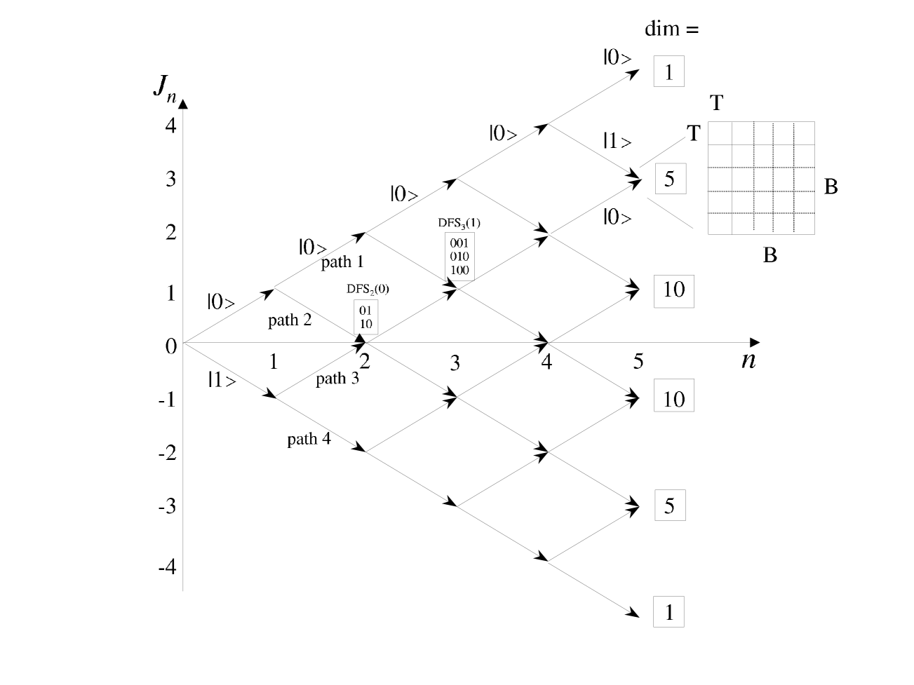
FIG. 1.: Weak collective decoherence. The horizontal axis is the number of qubits; the vertical axis is the number of $0$’s minus the number of $1$’s in each state ($J_{n}$). Each state in the standard basis thus corresponds to a path from the origin following the indicated arrows. The dimension of a DFS corresponds to the multiple pathways through which one can arrive at the same $J_{n}$. The insert shows the matrix structure of operators acting on DFS${}_{5}(3)$, in terms of Top (T) and Bottom (B) states. Note that there is only one T-state entering DFS${}_{5}(3)$, whence the action of exchange is represented by a $1\times 1$ block.

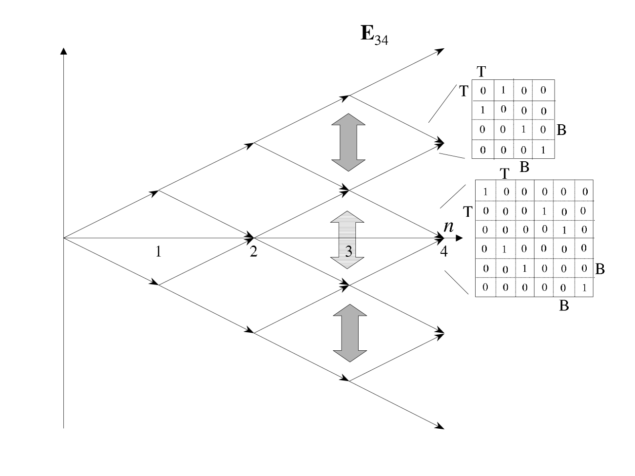
FIG. 2.: Action of exchange is to simultaneously flip different paths. Matrices are the representations of ${\bf E}_{34}$ on DFS${}_{4}(0)$ (lower) and DFS${}_{4}(2)$ (upper).

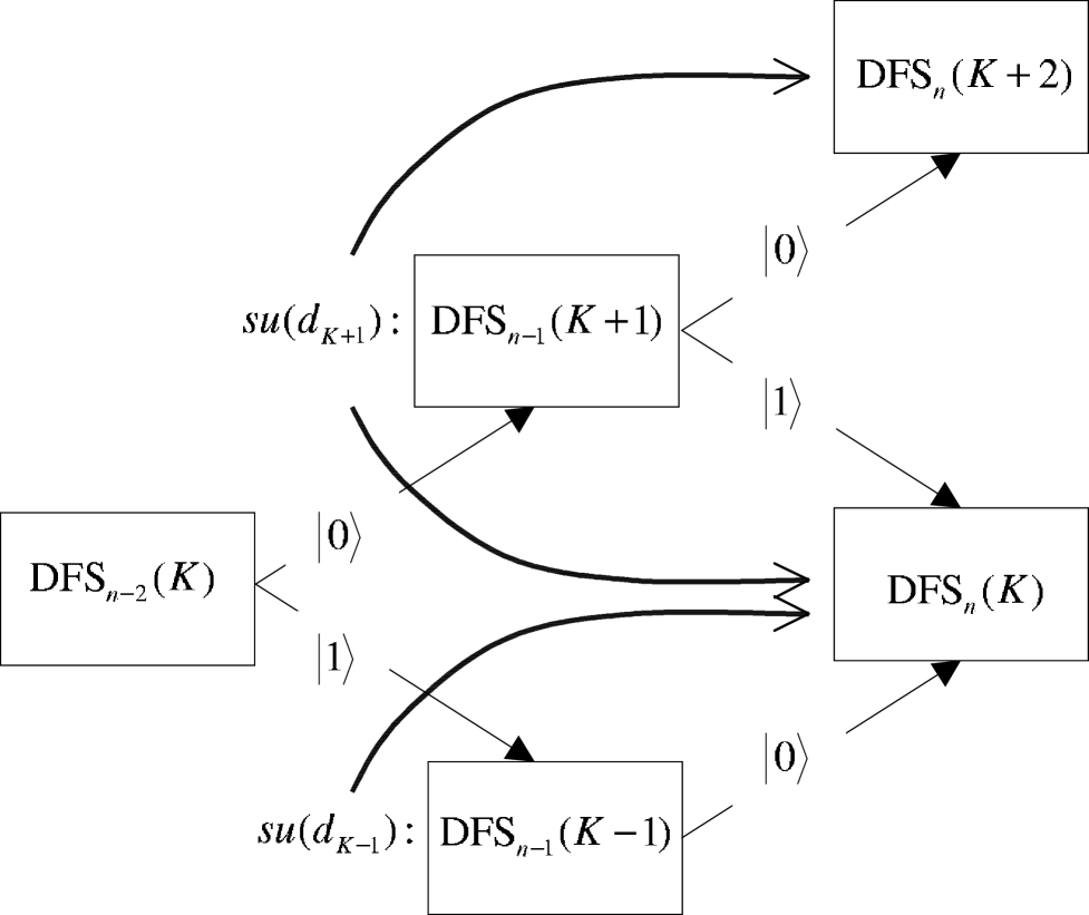
FIG. 3.: The structure of the pathways connecting adjacent DFSs in the weak collective decoherence case. The action of the different $su$ Lie algebras is indicated by heavy arrows.

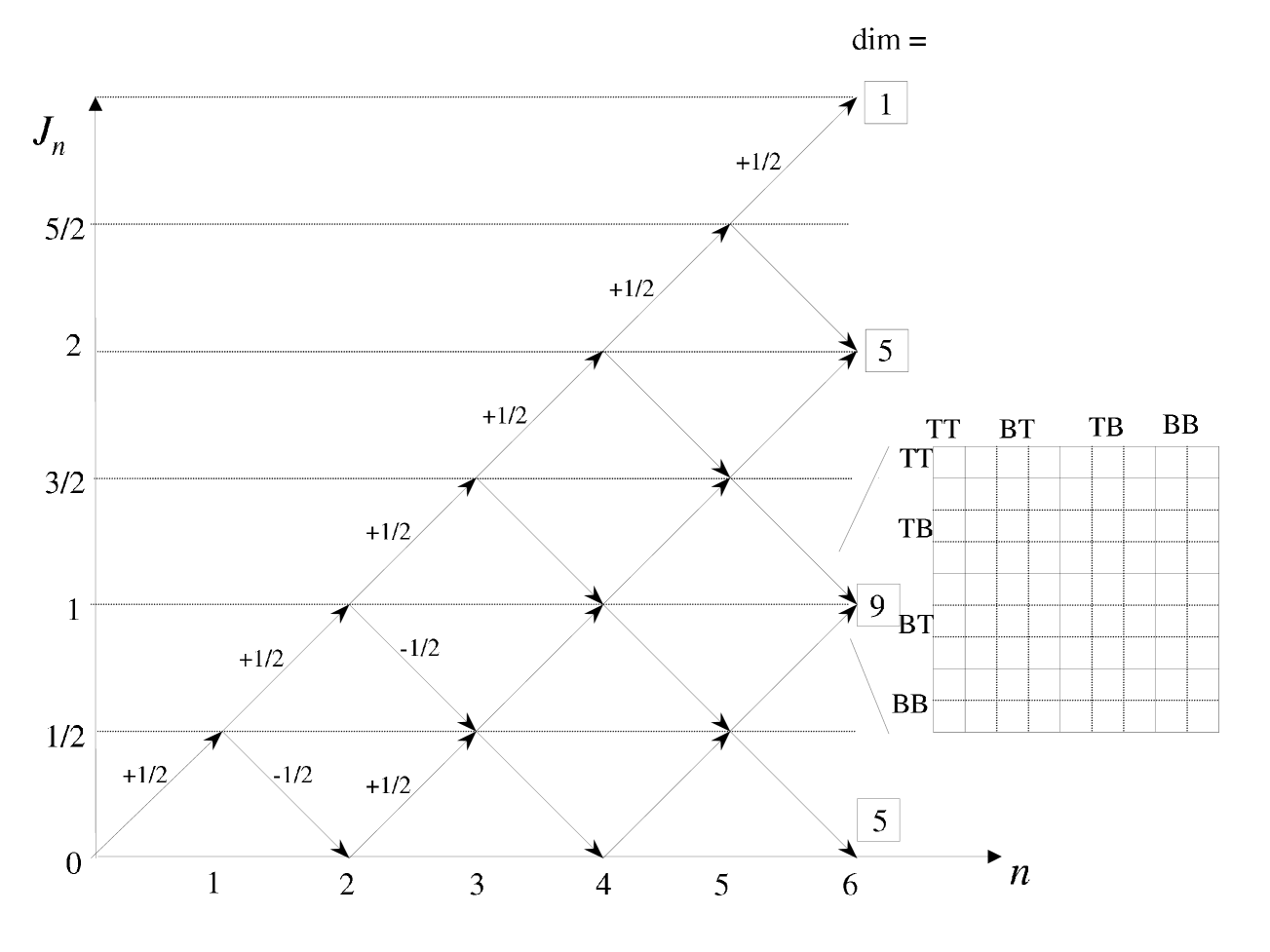
FIG. 4.: Strong collective decoherence. The horizontal axis is the number of qubits and the vertical axis is the total angular momentum. Each state in the DFS is represented by a pathway from the origin along the arrows as indicated. The insert shows the matrix structure of operators acting on DFS${}_{6}(1)$, in terms of TT, TB, BT, and BB-states.

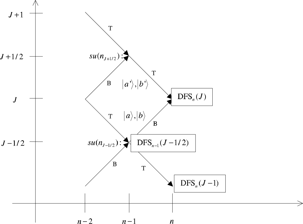
FIG. 5.: Scheme to visualize the inductive proof for the strong collective decoherence case. TB- and BT-states of DFS${}_{n}(J)$ are indicated. $su(n_{J-1/2})$ acts on DFS${}_{n}(J-1)$ and DFS${}_{n}(J)$ via DFS${}_{n-1}(J-1/2)$. See text for details.

REFERENCES

- [1] P.W. Shor, in Proceedings of the 35th Annual Symposium on the Foundations of Computer Science, edited by S. Goldwasser (IEEE Computer Society, Los Alamitos, CA, 1994), p. 124.
- [2] L.K. Grover, Phys. Rev. Lett. 79, 325 (1997), LANL preprint quant-ph/9706033.
- [3] C.H. Bennett, G. Brassard, C. Crepeau, R. Jozsa, A. Peres and W.K. Wootters, Phys. Rev. Lett. 70, 1895 (1993).
- [4] C.H. Bennett and P.W. Shor, IEEE Trans. Info. Theory 44, 2724 (1998).
- [5] Abbreviations frequently used in this paper are: QECC = quantum error correcting code, DFS = decoherence-free subsystem (or subspace, if no confusion can arise), WCD/SCD = weak/strong collective decoherence, irrep = irreducible representation.
- [6] P.W. Shor, Phys. Rev. A 52, 2493 (1995).
- [7] A.M. Steane, Phys. Rev. Lett. 77, 793 (1996).
- [8] E. Knill and R. Laflamme, Phys. Rev. A 55, 900 (1997).
- [9] D. Gottesman, Phys. Rev. A 54, 1862 (1997), LANL preprint quant-ph/9604038.
- [10] D. Aharonov and M. Ben-Or, in Proceedings of 29th Annual ACM Symposium on Theory of Computing (STOC) (ACM, New York, NY, 1997), p. 46, LANL preprint quant-ph/9611025.
- [11] R. L. E. Knill and W. Zurek, Science 279, 342 (1998).
- [12] J. Preskill, Proc. R. Soc. 454, 385 (1998).
- [13] G. Palma, K. Suominen, and A. Ekert, Proc. Roy. Soc. London Ser. A 452, 567 (1996).
- [14] L.-M. Duan and G.-C. Guo, Phys. Rev. Lett. 79, 1953 (1997), LANL preprint quant-ph/9703040.
- [15] L.-M Duan and G.-C. Guo, Phys. Rev. A 57, 737 (1998).
- [16] P. Zanardi and M. Rasetti, Mod. Phys. Lett. B 11, 1085 (1997), LANL preprint quant-ph/9710041.
- [17] P. Zanardi, Phys. Rev. A 56, 4445 (1997), LANL preprint quant-ph/9708042.
- [18] P. Zanardi and M. Rasetti, Phys. Rev. Lett. 79, 3306 (1997), LANL preprint quant-ph/9705044.
- [19] P. Zanardi, Phys. Rev. A 57, 3276 (1998), LANL preprint quant-ph/9705045.
- [20] P. Zanardi and M. Rasetti, Phys. Rev. A 57, 3276 (1998), LANL preprint quant-ph/9705045.
- [21] D.A. Lidar, I.L. Chuang, and K.B. Whaley, Phys. Rev. Lett. 81, 2594 (1998), LANL preprint quant-ph/9807004.
- [22] D.A. Lidar, D. Bacon, and K.B. Whaley, Phys. Rev. Lett. 82, 4556 (1999), LANL preprint quant-ph/9809081.
- [23] D.A. Lidar, D. Bacon, J. Kempe, and K.B. Whaley, Universal Fault Tolerant Quantum Computation on a Class of Decoherence-Free Subspaces Without Spatial Symmetry, LANL preprint quant-ph/9908064.
- [24] D. Bacon, D.A. Lidar, K.B. Whaley, Phys. Rev. A 60, 1944 (1999), LANL preprint quant-ph/9902041.
- [25] D.A. Lidar, D. Bacon, J. Kempe and K.B. Whaley, Phys. Rev. A 61, 052307 (2000), LANL Report No. quant-ph/9907096.
- [26] M. Durdevich, H.E. Makaruk, R.Owczarek, Generalized Noiseless Quantum Codes utilizing Quantum Enveloping Algebras, LANL preprint quant-ph/0003134.
- [27] P. Zanardi and F. Rossi, Phys. Rev. Lett. 81, 4572 (1998), LANL preprint quant-ph/9804016.
- [28] P. Zanardi and F. Rossi, Phys. Rev. B 59, 8170 (1999), LANL preprint quant-ph/9808036.
- [29] P. Zanardi, Phys. Rev. A 60, R729 (1999), LANL preprint quant-ph/9901047.
- [30] A. Beige, D. Braun, and P.L. Knight, Driving Atoms Into Decoherence-Free States, LANL preprint quant-ph/9912004.
- [31] A. Beige, D. Braun, B.Tregenna, and P.L. Knight, Quantum Computing Using Dissipation, LANL preprint quant-ph/0004043.
- [32] D. Bacon, J. Kempe, D.A. Lidar, K.B. Whaley, Universal Fault-Tolerant Computation on Decoherence Free Subspaces, LANL preprint quant-ph/9909058.
- [33] D. Deutsch, A. Barenco and A. Ekert, Proc. Roy. Soc. London Ser. A 449, 669 (1995).
- [34] A. Barenco, Proc. Roy. Soc. London Ser. A 449, 679 (1995).
- [35] D. P. DiVincenzo, Phys. Rev. A 51, 1015 (1995).
- [36] S. Lloyd, Phys. Rev. A 75, 346 (1995).
- [37] T. Sleator and H. Weinfurter, Phys. Rev. Lett. 74, 4087 (1995).
- [38] L. Duan and G. Guo, Phys. Lett. A 255, 209 (1999), LANL Report No. quant-ph/9809057.
- [39] E. Knill, R. Laflamme and L. Viola, Phys. Rev. Lett. 84, 2525 (2000), LANL preprint quant-ph/9909094.
- [40] L. Viola, E. Knill, and S. Lloyd, Dynamical Generation of Noiseless Quantum Subsystems, LANL preprint quant-ph/0002072.
- [41] H. Carmichael, An Open Systems Approach to Quantum Optics, No. m18 in Lecture notes in physics (Springer-Verlag, Berlin, 1993).
- [42] P. Zanardi, Stabilizing Quantum Information, LANL preprint quant-ph/9910016.
- [43] D. Gottesman, Phys. Rev. A 57, 127 (1997), LANL Report No. quant-ph/9702029.
- [44] G. Lindblad, Commun. Math. Phys. 48, 119 (1976).
- [45] R. Alicki and K. Lendi, Quantum Dynamical Semigroups and Applications, No. 286 in Lecture Notes in Physics (Springer-Verlag, Berlin, 1987).
- [46] S. De Filippo, Quantum Computation by Decoherence Free Operator Algebras, LANL preprint quant-ph/9910005.
- [47] N.P. Landsman, Lecture Notes on C∗-algebras, Hilbert C∗-modules and Quantum Mechanics, LANL preprint math-ph/9807030.
- [48] K. Kraus, States, Effects and Operations, Fundamental Notions of Quantum Theory (Academic, Berlin, 1983).
- [49] J.P. Paz and W.H. Zurek, Proc. Roy. Soc. London Ser. A 454, 355 (1998), LANL Report No. quant-ph/9707049.
- [50] D. Aharonov and M. Ben-Or, Fault-tolerant Quantum Computation with constant error rate, LANL preprint quant-ph/9906129.
- [51] D. Barenco, C. H. Bennett, R. Cleve, D. P. DiVincenzo, N. Margolus, P. Shor, T. Sleator, J. Smolin, and H. Weinfurter, Phys. Rev. A 52, 3457 (1995), LANL preprint quant-ph/9503016.
- [52] R. H. Dicke, Phys. Rev. 93, 99 (1954).
- [53] L. Mandel and E. Wolf, Optical coherence and quantum optics (Cambridge University Press, New York, 1995).
- [54] D. P. DiVincenzo, G. Burkard, D. Loss, E. V. Sukhorukov, in Quantum Mesoscopic Phenomena and Mesoscopic Devices in Microelectronics., edited by I. O. Kulk and R. Ellialtioglu (NATO Advanced Study Institute, Turkey, 1999), LANL preprint cond-mat/9911245.
- [55] R. Laflamme, C. Miquel, J.P. Paz and W.H. Zurek, Phys. Rev. Lett. 77, 198 (1996), LANL Report No. quant-ph/9602019.
- [56] D. Gottesman, Fault-Tolerant Quantum Computation with Local Gates, LANL Report No. quant-ph/9903099.
- [57] R.N. Cahn, Semi-Simple Lie Algebras and Their Representations (Benjamin/Cummings, Reading, 1984), available online at http://www-physics.lbl.gov/ rncahn/book.html.