Further Contents of Einstein’s E = mc²

Abstract

The energy-mass content of Einstein’s $E=mc^{2}$ is well known. For a fixed value of mass, $E=mc^{2}$ is an energy-momentum relation which takes the form $E=\sqrt{m^{2}+p^{2}}$. This relation was formulated in 1905 for point particles. Since then, particles have become more complicated. They have internal space-time structures. Massive particles carry the package of internal variables including mass, spin and quarks, while massless particles have the package containing helicity, gauge variables, and partons. The question then is whether these two different packages of variables can be unified into one single covariant package as $E=mc^{2}$ does for the energy-momentum relations for massive and massless particles. The answer to this question is YES.

I Introduction

If the momentum of a particle is much smaller than its mass, the energy-momentum relation is $E=p^{2}/2m+mc^{2}$. If the momentum is much larger than the mass, the relation is $E=cp$. These two different relations can be combined into one covariant formula $E=\sqrt{m^{2}+p^{2}}$. This aspect of Einstein’s $E=mc^{2}$ is also well known.

In addition, particles have internal space-time variables. Massive particles have spins while massless particles have their helicities and gauge variables. Our first question is whether this aspect of space-time variables can be unified into one covariant concept. The answer to this question is Yes. Wigner’s little group does the job. In addition, particles can have space-time extensions. For instance, in the quark model, particles are bound states of quarks. These bound states are called hadrons. However, the hadrons appear as a collection of partons when they move with speed close to the velocity of light. Quarks and partons seem to have quite distinct properties. In this report, we resolve this quark/parton puzzle. We shall see that the quark model and parton model are two different manifestations of the same covariant quantity.

By “further contents” of Einstein’s $E=mc^{2}$, we mean that the internal space-time structures of massive and massless particles can be unified into one covariant package, as $E=\sqrt{m^{2}+p^{2}}$ does for the energy-momentum relation. The mathematical framework of this program was developed by Eugene Wigner in 1939 [1]. He constructed maximal subgroups of the Lorentz group whose transformations will leave the four-momentum of a given particle invariant. These groups are known as Wigner’s little groups. Thus, the transformations of the little groups change the internal space-time variables the particle. The little group is a covariant entity and takes different forms for the particles moving with different speeds.

As for the relativistic extended particles, the most efficient approach is to construct the representations of the little groups using the wave functions which can be Lorentz-boosted. This means that we have to construct wave functions which are consistent with all known rules of quantum mechanics. It is possible to construct harmonic oscillator wave functions which satisfy these conditions. We can then take the low-speed and high-speed limits of the covariant harmonic oscillator wave functions for the quark model and the parton model respectively.

The scope of this report is summarized in Table I. We first use the little groups to unify the spin variables for massive and massless particles. We then study the Lorentz-group contents of relativistic extended hadrons to establish the quark-parton covariance.

TABLE I.: Further contents of Einstein’s $E=mc^{2}$. Massive and massless particles have different energy-momentum relations. Einstein’s special relativity gives one relation for both. Wigner’s little group unifies the internal space-time symmetries for massive and massless particles. The quark model and the parton model can also be combined into one covariant model.

	Massive, Slow	COVARIANCE	Massless, Fast
Energy-		Einstein’s
Momentum	$E=p^{2}/2m$	$E=[p^{2}+m^{2}]^{1/2}$	$E=cp$
Internal	$S_{3}$		$S_{3}$
space-time		Wigner’s
symmetry	$S_{1},S_{2}$	Little Group	Gauge Transformations
Relativistic
Extended	Quark Model	Covariant Model of Hadrons	Partons
Particles

In Sec. II, we construct the little groups from their definition that their transformations leave the four-momentum of a given particle invariant. In Sec. III, we discuss in detail how the little group for a massless particle can be obtained as the zero-mass/infinite-momentum limit of the little group for the massive particle. The covariant oscillator formalism is spelled out in detail in Sec. IV. In Sec. V, we use the oscillator wave function to show that quarks and partons are the same particles.

II Formulation of the Problem

The space-time symmetry of relativistic particles is dictated by the Poincaré group [1]. The Poincaré group is the group of inhomogeneous Lorentz transformations, namely Lorentz transformations preceded or followed by space-time translations. Thus, the Poincaré group is a semi-direct product of the Lorentz and translation groups. The two Casimir operators of this group correspond to the (mass)² and (spin)² of a given particle. Indeed, the particle mass and its spin magnitude are Lorentz-invariant quantities.

The question then is how to construct the representations of the Lorentz group which are relevant to physics. For this purpose, Wigner in 1939 studied the maximal subgroups of the Lorentz group whose transformations leave the four-momentum of a given free particle [1]. These subgroups are called the little groups. Since the little group leaves the four-momentum invariant, it governs the internal space-time symmetries of relativistic particles. Wigner shows in his paper that the internal space-time symmetries of massive and massless particles are dictated by the little groups which are locally isomorphic to the three-dimensional rotation group and the two-dimensional Euclidean groups respectively.

The group of Lorentz transformations consists of three boosts and three rotations. The rotations therefore constitute a subgroup of the Lorentz group. If a massive particle is at rest, its four-momentum is invariant under rotations. Thus the little group for a massive particle at rest is the three-dimensional rotation group. Then what is affected by the rotation? The answer to this question is very simple. The particle in general has its spin. The spin orientation is going to be affected by the rotation! If we use the four-vector coordinate $(x,y,z,t)$, the four-momentum vector for the particle at rest is $(0,0,0,m)$, and the three-dimensional rotation group leaves this four-momentum invariant. This little group is generated by

$$J_{1}=\pmatrix{0&0&0&0\cr 0&0&-i&0\cr 0&i&0&0\cr 0&0&0&0},\qquad J_{2}=\pmatrix{0&0&i&0\cr 0&0&0&0\cr-i&0&0&0\cr 0&0&0&0},\qquad J_{3}=\pmatrix{0&-i&0&0\cr i&0&0&0\cr 0&0&0&0\cr 0&0&0&0}.$$ (1)

These are essentially the generators of the three-dimensional rotation group. They satisfy the commutation relations:

$$[J_{i},J_{j}]=i\epsilon_{ijk}J_{k}.$$ (2)

If the rest-particle is boosted along the $z$ direction, it will pick up a non-zero momentum component along the same direction. The above generators will also be boosted. The boost will take the form of conjugation by the boost matrix

$$B=\pmatrix{1&0&0&0\cr 0&1&0&0\cr 0&0&\cosh\eta&\sinh\eta\cr 0&0&\sinh\eta&\cosh\eta}.$$ (3)

This boost will not change the commutation relations of Eq.(2) for $O(3)$, and the boosted little group will still leave the boosted four-momentum invariant. Thus, the little group of a moving massive particle is still $O(3)$-like.

It is not possible to bring a massless particle to its rest frame. In his 1939 paper [1], Wigner observed that the little group for a massless particle moving along the $z$ axis is generated by the rotation generator around the $z$ axis, namely $J_{3}$ of Eq.(1), and two other generators which take the form

$$N_{1}=\pmatrix{0&0&-i&i\cr 0&0&0&0\cr i&0&0&0\cr i&0&0&0},\quad N_{2}=\pmatrix{0&0&0&0\cr 0&0&-i&i\cr 0&i&0&0\cr 0&i&0&0}.$$ (4)

If we use $K_{i}$ for the boost generator along the i-th axis, these matrices can be written as

$$N_{1}=K_{1}-J_{2},\qquad N_{2}=K_{2}+J_{1},$$ (5)

with

$$K_{1}=\pmatrix{0&0&0&i\cr 0&0&0&0\cr 0&0&0&0\cr i&0&0&0},\qquad K_{2}=\pmatrix{0&0&0&0\cr 0&0&0&i\cr 0&0&0&0\cr 0&i&0&0}.$$ (6)

The generators $J_{3},N_{1}$ and $N_{2}$ satisfy the following set of commutation relations.

$$[N_{1},N_{2}]=0,\qquad[J_{3},N_{1}]=iN_{2},\qquad[J_{3},N_{2}]=-iN_{1}.$$ (7)

In order to understand the mathematical basis of the above commutation relations, let us consider transformations on a two-dimensional plane with the $xy$ coordinate system. We can then make rotations around the origin and translations along the $x$ and $y$ directions. If we write these generators as $L,P_{x}$ and $P_{y}$ respectively, they satisfy the commutation relations [2]

$$[P_{x},P_{y}]=0,\qquad[L,P_{x}]=iP_{y},\qquad[L,P_{y}]=-iP_{x}.$$ (8)

This is a closed set of commutation relations for the generators of the $E(2)$ group. If we replace $N_{1}$ and $N_{2}$ of Eq.(7) by $P_{x}$ and $P_{y}$, and $J_{3}$ by $L$, the commutations relations for the generators of the $E(2)$-like little group becomes those for the $E(2)$-like little group. This is precisely why we say that the little group for massless particles are like $E(2)$.

It is not difficult to associate the rotation generator $J_{3}$ with the helicity degree of freedom of the massless particle. Then what physical variable is associated with the $N_{1}$ and $N_{2}$ generators? Indeed, Wigner was the one who discovered the existence of these generators, but did not give any physical interpretation to these translation-like generators. For this reason, for many years, only those representations with the zero-eigenvalues of the $N$ operators were thought to be physically meaningful representations [3]. It was not until 1971 when Janner and Janssen reported that the transformations generated by these operators are gauge transformations [4, 5]. The role of this translation-like transformation has also been studied for spin-1/2 particles, and it was concluded that the polarization of neutrinos is due to gauge invariance [6, 7].

III Contraction of O(3)-like to E(2)-like Little Groups

The $O(3)$-like little group remains $O(3)$-like when the particle is Lorentz-boosted. Then, what happens when the particle speed becomes the speed of light? The energy-momentum relation $E=\sqrt{m^{2}+p^{2}}$ become $E=p$. Is there then a limiting case of the $O(3)$-like little group? Since those little groups are like the three-dimensional rotation group and the two-dimensional Euclidean group respectively, we are first interested in whether $E(2)$ can be obtained from $O(3)$. This will then give a clue to obtaining the $E(2)$-like little group as a limiting case of $O(3)$-like little group. With this point in mind, let us look into this geometrical problem.

In 1953, Inonu and Wigner formulated this problem as the contraction of $O(3)$ to $E(2)$ [8]. Let us see what they did. We always associate the three-dimensional rotation group with a spherical surface. Let us consider a circular area of radius 1 kilometer centered on the north pole of the earth. Since the radius of the earth is more than 6,450 times longer, the circular region appears flat. Thus, within this region, we use the $E(2)$ symmetry group for this region. The validity of this approximation depends on the ratio of the two radii.

How about then the little groups which are isomorphic to $O(3)$ and $E(2)$? It is reasonable to expect that the $E(2)$-like little group be obtained as a limiting case for of the $O(3)$-like little group for massless particles. In 1981, it was observed by Ferrara and Savoy that this limiting process is the Lorentz boost [9]. In 1983, using the same limiting process as that of Ferrara and Savoy, Han et al showed that transverse rotation generators become the generators of gauge transformations in the limit of infinite momentum and/or zero mass [10].

Let us see how this happens. The $J_{3}$ operator of Eq.(1), which generates rotations around the $z$ axis, is not affected by the boost conjugation by the $B$ matrix of Eq.(3). On the other hand, the $J_{1}$ and $J_{2}$ matrices become

$$N_{1}=e^{-\eta}B^{-1}J_{2}B,\qquad N_{2}=-e^{-\eta}B^{-1}J_{1}B,$$ (9)

and they become $N_{1}$ and $N_{2}$ given in Eq.(4). The generators $N_{1}$ and $N_{2}$ are the contracted $J_{2}$ and $J_{1}$ respectively in the infinite-momentum/zero-mass limit. In 1987, Kim and Wigner studied this problem in more detail and showed that the little group for massless particles is the cylindrical group which is isomorphic to the $E(2)$ group [11]. Their work is summarized in Fig. 1.

This completes the second row in Table I, where Wigner’s little group unifies the internal space-time symmetries of massive and massless particles. The transverse components of the rotation generators become generators of gauge transformations in the infinite-momentum/zero-mass limit.

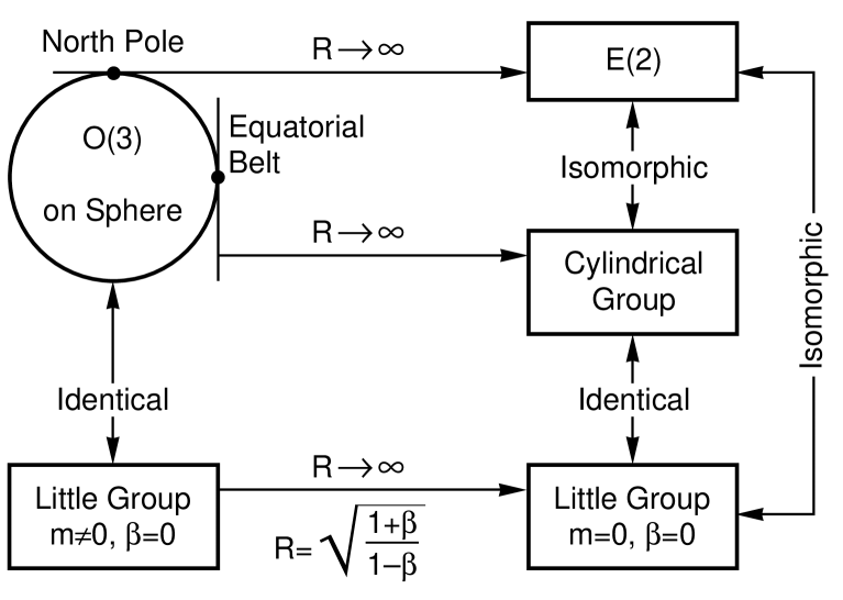
FIG. 1.: Contraction of $O(3)$ to $E(2)$ and to the cylindrical group, and contraction of the $O(3)$-like little group to the $E(2)$-like little group. The correspondence between $E(2)$ and the $E(2)$-like little group is isomorphic but not identical. The cylindrical group is identical to the $E(2)$-like little group. The Lorentz boost of the $O(3)$-like little group for a massive particle is the same as the contraction of $O(3)$ to the cylindrical group.

IV Covariant Harmonic Oscillators

We are now interested in constructing the third row in Table I. As we promised in Sec. I, we will be dealing with hadrons which are bound states of quarks with space-time extensions. For this purpose, we need a set of covariant wave functions consistent with the existing laws of quantum mechanics, including of course the uncertainty principle and probability interpretation. The first wave function which comes to our mind is the harmonic oscillator wave function. If we are interested in Lorentz-transforming them, the most straight-forward method is to construct representations of the Poincaré group using harmonic oscillators wave functions [12, 13, 14, 2].

In this report, we start with the Lorentz-invariant differential equation of Feynman, Kislinger, and Ravndal [15]. It is a linear partial differential equation which has many different solutions depending on boundary conditions. Unlike in the case of Feynman et al., we use normalizable wave functions which constitute a representation of the $O(3)$-like little group [2].

Let us consider a bound state of two particles. For convenience, we shall call the bound state the hadron, and call its constituents quarks. Then there is a Bohr-like radius measuring the space-like separation between the quarks. There is also a time-like separation between the quarks, and this variable becomes mixed with the longitudinal spatial separation as the hadron moves with a relativistic speed. There are no quantum excitations along the time-like direction. On the other hand, there is the time-energy uncertainty relation which allows quantum transitions. It is possible to accommodate these aspect within the framework of the present form of quantum mechanics. The uncertainty relation between the time and energy variables is the c-number relation [16], which does not allow excitations along the time-like coordinate. We shall see that the covariant harmonic oscillator formalism accommodates this narrow window in the present form of quantum mechanics.

For a hadron consisting of two quarks, we can consider their space-time positions $x_{a}$ and $x_{b}$, and use the variables

$$X=(x_{a}+x_{b})/2,\qquad x=(x_{a}-x_{b})/2\sqrt{2}.$$ (10)

The four-vector $X$ specifies where the hadron is located in space and time, while the variable $x$ measures the space-time separation between the quarks. In the convention of Feynman et al. [15], the internal motion of the quarks bound by a harmonic oscillator potential of unit strength can be described by the Lorentz-invariant equation

$${1\over 2}\left\{x^{2}_{\mu}-{\partial^{2}\over\partial x_{\mu}^{2}}\right\}\psi(x)=\lambda\psi(x).$$ (11)

It is now possible to construct a representation of the Poincaré group from the solutions of the above differential equation [2].

The coordinate $X$ is associated with the overall hadronic four-momentum, and the space-time separation variable $x$ dictates the internal space-time symmetry or the $O(3)$-like little group. Thus, we should construct the representation of the little group from the solutions of the differential equation in Eq.(11). If the hadron is at rest, we can separate the $t$ variable from the equation. For this variable we can assign the ground-state wave function to accommodate the c-number time-energy uncertainty relation [16]. For the three space-like variables, we can solve the oscillator equation in the spherical coordinate system with usual orbital and radial excitations. This will indeed constitute a representation of the $O(3)$-like little group for each value of the mass. The solution should take the form

$$\psi(x,y,z,t)=\psi(x,y,z)\left({1\over\pi}\right)^{1/4}\exp\left(-t^{2}/2\right),$$ (12)

where $\psi(x,y,z)$ is the wave function for the three-dimensional oscillator with appropriate angular momentum quantum numbers. Indeed, the above wave function constitutes a representation of Wigner’s $O(3)$-like little group for a massive particle [2].

Since the three-dimensional oscillator differential equation is separable in both spherical and Cartesian coordinate systems, $\psi(x,y,z)$ consists of Hermite polynomials of $x,y$, and $z$. If the Lorentz boost is made along the $z$ direction, the $x$ and $y$ coordinates are not affected, and can be temporarily dropped from the wave function. The wave function of interest can be written as

$$\psi^{n}(z,t)=\left({1\over\pi}\right)^{1/4}\exp\pmatrix{-t^{2}/2}\psi_{n}(z),$$ (13)

with

$$\psi^{n}(z)=\left({1\over\pi n!2^{n}}\right)^{1/2}H_{n}(z)\exp(-z^{2}/2),$$ (14)

where $\psi^{n}(z)$ is for the $n$-th excited oscillator state. The full wave function $\psi^{n}(z,t)$ is

$$\psi^{n}_{0}(z,t)=\left({1\over\pi n!2^{n}}\right)^{1/2}H_{n}(z)\exp\left\{-{1\over 2}\left(z^{2}+t^{2}\right)\right\}.$$ (15)

The subscript $0$ means that the wave function is for the hadron at rest. The above expression is not Lorentz-invariant, and its localization undergoes a Lorentz squeeze as the hadron moves along the $z$ direction [2].

It is convenient to use the light-cone variables to describe Lorentz boosts. The light-cone coordinate variables are

$$u=(z+t)/\sqrt{2},\qquad v=(z-t)/\sqrt{2}.$$ (16)

In terms of these variables, the Lorentz boost along the $z$ direction,

$$\pmatrix{z^{\prime}\cr t^{\prime}}=\pmatrix{\cosh\eta&\sinh\eta\cr\sinh\eta&\cosh\eta}\pmatrix{z\cr t},$$ (17)

takes the simple form

$$u^{\prime}=e^{\eta}u,\qquad v^{\prime}=e^{-\eta}v,$$ (18)

where $\eta$ is the boost parameter and is $\tanh^{-1}(v/c)$. Indeed, the $u$ variable becomes expanded while the $v$ variable becomes contracted. This is the squeeze mechanism illustrated discussed extensively in the literature [17, 18].

The wave function of Eq.(15) can be written as

$$\psi^{n}_{o}(z,t)=\psi^{n}_{0}(z,t)=\left({1\over\pi n!2^{n}}\right)^{1/2}H_{n}\left((u+v)/\sqrt{2}\right)\exp\left\{-{1\over 2}(u^{2}+v^{2})\right\}.$$ (19)

If the system is boosted, the wave function becomes

$$\psi^{n}_{\eta}(z,t)=\left({1\over\pi n!2^{n}}\right)^{1/2}H_{n}\left((e^{-\eta}u+e^{\eta}v)/\sqrt{2}\right)\times\exp\left\{-{1\over 2}\left(e^{-2\eta}u^{2}+e^{2\eta}v^{2}\right)\right\}.$$ (20)

In both Eqs. (19) and (20), the localization property of the wave function in the $uv$ plane is determined by the Gaussian factor, and it is sufficient to study the ground state only for the essential feature of the boundary condition. The wave functions in Eq.(19) and Eq.(20) then respectively become

$$\psi_{0}(z,t)=\left({1\over\pi}\right)^{1/2}\exp\left\{-{1\over 2}(u^{2}+v^{2})\right\}.$$ (21)

If the system is boosted, the wave function becomes

$$\psi_{\eta}(z,t)=\left({1\over\pi}\right)^{1/2}\exp\left\{-{1\over 2}\left(e^{-2\eta}u^{2}+e^{2\eta}v^{2}\right)\right\}.$$ (22)

We note here that the transition from Eq.(21) to Eq.(22) is a squeeze transformation. The wave function of Eq.(21) is distributed within a circular region in the $uv$ plane, and thus in the $zt$ plane. On the other hand, the wave function of Eq.(22) is distributed in an elliptic region. This is how the wave function is Lorentz-boosted.

V Feynman’s Parton Picture

It is safe to believe that hadrons are quantum bound states of quarks having localized probability distribution. As in all bound-state cases, this localization condition is responsible for the existence of discrete mass spectra. The most convincing evidence for this bound-state picture is the hadronic mass spectra which are observed in high-energy laboratories [2, 15]. However, this picture of bound states is applicable only to observers in the Lorentz frame in which the hadron is at rest. How would the hadrons appear to observers in other Lorentz frames?

In 1969, Feynman observed that a fast-moving hadron can be regarded as a collection of many “partons” whose properties do not appear to be identical to those of quarks [19]. For example, the number of quarks inside a static proton is three, while the number of partons in a rapidly moving proton appears to be infinite. The question then is how the proton looking like a bound state of quarks to one observer can appear different to an observer in a different Lorentz frame? Feynman made the following systematic observations.

• The picture is valid only for hadrons moving with velocity close to that of light.

• The interaction time between the quarks becomes dilated, and partons behave as free independent particles.

• The momentum distribution of partons becomes widespread as the hadron moves very fast.

• The number of partons seems to be infinite or much larger than that of quarks.

Because the hadron is believed to be a bound state of two or three quarks, each of the above phenomena appears as a paradox, particularly b) and c) together. We would like to resolve this paradox using the covariant harmonic oscillator formalism.

For this purpose, we need a momentum-energy wave function. If the quarks have the four-momenta $p_{a}$ and $p_{b}$, we can construct two independent four-momentum variables [15]

$$P=p_{a}+p_{b},\qquad q=\sqrt{2}(p_{a}-p_{b}).$$ (23)

The four-momentum $P$ is the total four-momentum and is thus the hadronic four-momentum. $q$ measures the four-momentum separation between the quarks.

We expect to get the momentum-energy wave function by taking the Fourier transformation of Eq.(22):

$$\phi_{\eta}(q_{z},q_{0})=\left({1\over 2\pi}\right)\int\psi_{\eta}(z,t)\exp{\left\{-i(q_{z}z-q_{0}t)\right\}}dxdt.$$ (24)

Let us now define the momentum-energy variables in the light-cone coordinate system as

$$q_{u}=(q_{0}-q_{z})/\sqrt{2},\qquad q_{v}=(q_{0}+q_{z})/\sqrt{2}.$$ (25)

In terms of these variables, the Fourier transformation of Eq.(24) can be written as

$$\phi_{\eta}(q_{z},q_{0})=\left({1\over 2\pi}\right)\int\psi_{\eta}(z,t)\exp{\left\{-i(q_{u}u+q_{v}v)\right\}}dudv.$$ (26)

The resulting momentum-energy wave function is

$$\phi_{\eta}(q_{z},q_{0})=\left({1\over\pi}\right)^{1/2}\exp\left\{-{1\over 2}\left(e^{-2\eta}q_{u}^{2}+e^{2\eta}q_{v}^{2}\right)\right\}.$$ (27)

Since we are using the harmonic oscillator, the mathematical form of the above momentum-energy wave function is identical to that of the space-time wave function. The Lorentz squeeze properties of these wave functions are also the same, as are indicated in Fig. 2. These squeeze transformations perfectly consistent with the algorithms of the Poincaré group [20].

When the hadron is at rest with $\eta=0$, both wave functions behave like those for the static bound state of quarks. As $\eta$ increases, the wave functions become continuously squeezed until they become concentrated along their respective positive light-cone axes. Let us look at the z-axis projection of the space-time wave function. Indeed, the width of the quark distribution increases as the hadronic speed approaches that of the speed of light. The position of each quark appears widespread to the observer in the laboratory frame, and the quarks appear like free particles.

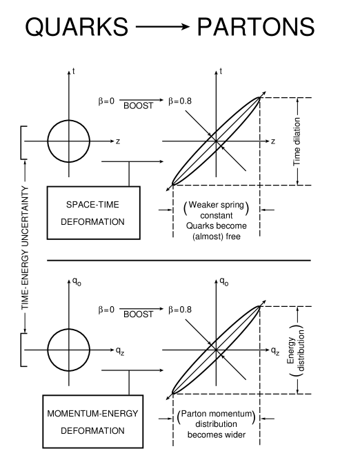
FIG. 2.: Lorentz-squeezed space-time and momentum-energy wave functions. As the hadron’s speed approaches that of light, both wave functions become concentrated along their respective positive light-cone axes. These light-cone concentrations lead to Feynman’s parton picture.

Furthermore, interaction time of the quarks among themselves become dilated. Because the wave function becomes wide-spread, the distance between one end of the harmonic oscillator well and the other end increases as is indicated in Fig. 2. This effect, first noted by Feynman [19], is universally observed in high-energy hadronic experiments. The period is oscillation is increases like $e^{\eta}$. On the other hand, the interaction time with the external signal, since it is moving in the direction opposite to the direction of the hadron, it travels along the negative light-cone axis. If the hadron contracts along the negative light-cone axis, the interaction time decreases by $e^{-\eta}$. The ratio of the interaction time to the oscillator period becomes $e^{-2\eta}$. The energy of each proton coming out of the Fermilab accelerator is $900GeV$. This leads the ratio to $10^{-6}$. This is indeed a small number. The external signal is not able to sense the interaction of the quarks among themselves inside the hadron.

The momentum-energy wave function is just like the space-time wave function. The longitudinal momentum distribution becomes wide-spread as the hadronic speed approaches the velocity of light. This is in contradiction with our expectation from nonrelativistic quantum mechanics that the width of the momentum distribution is inversely proportional to that of the position wave function. Our expectation is that if the quarks are free, they must have their sharply defined momenta, not a wide-spread distribution. This apparent contradiction presents to us the following two fundamental questions:

• . If both the spatial and momentum distributions become widespread as the hadron moves, and if we insist on Heisenberg’s uncertainty relation, is Planck’s constant dependent on the hadronic velocity?

• . Is this apparent contradiction related to another apparent contradiction that the number of partons is infinite while there are only two or three quarks inside the hadron?

The answer to the first question is “No”, and that for the second question is “Yes”. Let us answer the first question which is related to the Lorentz invariance of Planck’s constant. If we take the product of the width of the longitudinal momentum distribution and that of the spatial distribution, we end up with the relation

$$<z^{2}><q_{z}^{2}>=(1/4)[\cosh(2\eta)]^{2}.$$ (28)

The right-hand side increases as the velocity parameter increases. This could lead us to an erroneous conclusion that Planck’s constant becomes dependent on velocity. This is not correct, because the longitudinal momentum variable $q_{z}$ is no longer conjugate to the longitudinal position variable when the hadron moves.

In order to maintain the Lorentz-invariance of the uncertainty product, we have to work with a conjugate pair of variables whose product does not depend on the velocity parameter. Let us go back to Eq.(25) and Eq.(26). It is quite clear that the light-cone variable $u$ and $v$ are conjugate to $q_{u}$ and $q_{v}$ respectively. It is also clear that the distribution along the $q_{u}$ axis shrinks as the $u$-axis distribution expands. The exact calculation leads to

$$<u^{2}><q_{u}^{2}>=1/4,\qquad<v^{2}><q_{v}^{2}>=1/4.$$ (29)

Planck’s constant is indeed Lorentz-invariant.

Let us next resolve the puzzle of why the number of partons appears to be infinite while there are only a finite number of quarks inside the hadron. As the hadronic speed approaches the speed of light, both the x and q distributions become concentrated along the positive light-cone axis. This means that the quarks also move with velocity very close to that of light. Quarks in this case behave like massless particles.

We then know from statistical mechanics that the number of massless particles is not a conserved quantity. For instance, in black-body radiation, free light-like particles have a widespread momentum distribution. However, this does not contradict the known principles of quantum mechanics, because the massless photons can be divided into infinitely many massless particles with a continuous momentum distribution.

Likewise, in the parton picture, massless free quarks have a wide-spread momentum distribution. They can appear as a distribution of an infinite number of free particles. These free massless particles are the partons. It is possible to measure this distribution in high-energy laboratories, and it is also possible to calculate it using the covariant harmonic oscillator formalism. We are thus forced to compare these two results. Indeed, according to Hussar’s calculation [21], the Lorentz-boosted oscillator wave function produces a reasonably accurate parton distribution.

Concluding Remarks

According to $E=mc^{2}$, the energy can be measured in kilograms. For instance, Americans in the United States consume approximately $300Kg$ of electrical energy per year. For a fixed value of mass, the formula becomes $E=\sqrt{m^{2}+p^{2}}$, which unifies the energy-momentum relation for massless particle and that for massive particle with low speed.

We note that particles these days carry additional dynamical variables and concept. They carry internal space-time variables such as spin, helicity, and gauge degree of freedom. Wigner’s little group unifies all these variables into a single covariant regime. In addition, some particles, called hadrons, have their internal space-time distributions. These composite particles appear as two different entities in quantum mechanics. We noted in this report that they also can be unified.

REFERENCES

- [1] E. P. Wigner, Ann. Math. 40, 149 (1939).
- [2] Y. S. Kim and M. E. Noz, Theory and Applications of the Poincaré Group (Reidel, Dordrecht, 1986).
- [3] S. Weinberg, Phys. Rev. 134, B882 (1964); ibid. 135, B1049 (1964).
- [4] A. Janner and T. Janssen, Physica 53, 1 (1971); ibid. 60, 292 (1972).
- [5] Y. S. Kim, in Symmetry and Structural Properties of Condensed Matter, Proceedings 4th International School of Theoretical Physics (Zajaczkowo, Poland), edited by T. Lulek, W. Florek, and B. Lulek (World Scientific, 1997).
- [6] D. Han, Y. S. Kim, and D. Son, Phys. Rev. D 26, 3717 (1982).
- [7] Y. S. Kim, in Quantum Systems: New Trends and Methods, Proceedings of the International Workshop (Minsk, Belarus), edited by Y. S. Kim, L. M. Tomil’chik, I. D. Feranchuk, and A. Z. Gazizov (World Scientific, 1997)
- [8] E. Inonu and E. P. Wigner, Proc. Natl. Acad. Sci. (U.S.) 39, 510 (1953).
- [9] S. Ferrara and C. Savoy, in Supergravity 1981, S. Ferrara and J. G. Taylor eds. (Cambridge Univ. Press, Cambridge, 1982), p. 151. See also P. Kwon and M. Villasante, J. Math. Phys. 29, 560 (1988); ibid. 30, 201 (1989). For an earlier paper on this subject, see H. Bacry and N. P. Chang, Ann. Phys. 47, 407 (1968).
- [10] D. Han, Y. S. Kim, and D. Son, Phys. Lett. B 131, 327 (1983). See also D. Han, Y. S. Kim, M. E. Noz, and D. Son, Am. J. Phys. 52, 1037 (1984).
- [11] Y. S. Kim and E. P. Wigner, J. Math. Phys. 28, 1175 (1987) and 32, 1998 (1991). See also Y. S. Kim and E. P. Wigner, J. Math. Phys. 31, 55 (1990).
- [12] P. A. M. Dirac, Proc. Roy. Soc. (London) A183, 284 (1945).
- [13] H. Yukawa, Phys. Rev. 91, 415 (1953).
- [14] M. Markov, Suppl. Nuovo Cimento 3, 760 (1956).
- [15] R. P. Feynman, M. Kislinger, and F. Ravndal, Phys. Rev. D 3, 2706 (1971).
- [16] P. A. M. Dirac, Proc. Roy. Soc. (London) A114, 243 and 710 (1927).
- [17] Y. S. Kim and M. E. Noz, Phys. Rev. D 8, 3521 (1973).
- [18] Y. S. Kim and M. E. Noz, Phase Space Picture of Quantum Mechanics (World Scientific, Singapore, 1991).
- [19] R. P. Feynman, in High Energy Collisions, Proceedings of the Third International Conference, Stony Brook, New York, edited by C. N. Yang et al. (Gordon and Breach, New York, 1969). See also J. D. Bjorken and E. A. Paschos, Phys. Rev. 185, 1975 (1969).
- [20] Y. S. Kim, Phys. Rev. Lett. 63, 348 (1989).
- [21] P. E. Hussar, Phys. Rev. D 23, 2781 (1981).