Sampling the canonical phase from phase-space functions

Abstract

We discuss the possibility of sampling exponential moments of the canonical phase from the $s$-parametrized phase space functions. We show that the sampling kernels exist and are well-behaved for any $s$ $>$ $-1$, whereas for $s$ $=$ $-1$ the kernels diverge in the origin. In spite of that we show that the phase space moments can be sampled with any predefined accuracy from the $Q$-function measured in the double-homodyne scheme with perfect detectors. We discuss the effect of imperfect detection and address sampling schemes using other measurable phase-space functions. Finally, we discuss the problem of sampling the canonical phase distribution itself.

I Introduction

Studying the role of phase in quantum mechanics has a long history (for a review on the phase concepts, see, e.g., [1]). Its importance in today’s problems is also apparent. For example, phase in atomic systems has recently been used for storing quantum information [2], and phase and photon number measurements have been considered as a basis in some quantum teleportation schemes [3]. Notwithstanding the various phase-dependent effects in quantum physics, phase itself has not been uniquely measured and its very definition as physical quantity has been subject to many disputes. Whereas for highly excited (quasi-classical) states different approaches give similar results, the various concepts differ in the phase properties of quantum states close to vacuum. Therefore the question has been arisen of what are the differences between these approaches and how relevant are they experimentally. In this paper we concentrate on the canonical phase and its relation to $s$-parametrized phase-space functions, with special emphasis on the measurability of its exponential moments by “weighted” averaging of measured phase space functions.

The canonical phase distribution $P(\varphi)$ of a radiation field mode (harmonic oscillator) prepared in a quantum state described by a density operator $\hat{\varrho}$ is defined by

$$P(\varphi)=(2\pi)^{-1}\langle\varphi|\hat{\varrho}|\varphi\rangle,$$ (1)

where the Fock state expansion of the (unnormalizable) phase states $|\varphi\rangle$ reads

$$|\varphi\rangle=\sum_{n=0}^{\infty}e^{in\varphi}|n\rangle.$$ (2)

Even though there has been no known experimental scheme that is directly governed by $P(\varphi)$, this distribution has very nice properties: it is non-negative, conjugated to the photon-number distribution (in the sense that a phase shifter shifts a phase distribution while a number shifter does not change it [4]), there exist number-phase uncertainty relations [5], and in comparison to other phase distributions, $P(\varphi)$ is the most sharp one.

The lack of direct experimental availability of $P(\varphi)$ has led us to the search of schemes for sampling the canonical phase statistics from quantities that can be measured directly [6, 7, 8]. In balanced homodyne detection (for a review on quantum state measurement using homodyning, see, e.g., [9]), the exponential moments $\Psi_{k}$ of the canonical phase,

$$\Psi_{k}=\int_{2\pi}d\varphi\,e^{ik\varphi}P(\varphi),\quad\Psi_{-k}=\Psi_{k}^{\ast},$$ (3)

can be sampled by integrating the measured quadrature-component statistics multiplied by well-behaved kernel functions [6, 7, 8]. An advantage of the method is that it applies to both the quantum regime and the classical regime in a unified way. Of course, the question has been as of whether or not it is possible to find other (and possibly better) measurement schemes suitable for sampling the exponential moments of the canonical phase.

It is well known that balanced double-homodyne detection (eight-port homodyning, [10]) provides us with a two dimensional set of data whose statistics correspond to a $s$-parametrized phase-space function $W_{s}(q,p)$ with $s$ $\!\leq$ $\!-1$ [11]. In this scheme, the limiting case of $s$ $\!=$ $\!-1$, which corresponds to the Husimi $Q$-function $Q(q,p)$ $\!=$ $\!W_{-1}(q,p)$, requires perfect detection, i.e., 100% detection efficiency. Having a sampling scheme leading from a measured $s$-parametrized phase-space function to the exponential canonical-phase moments would be the most direct method of measuring the exponential moments of the canonical phase. Since each measurement event $(q,p)$ already yields a phase value Arg$(q+ip)$, the measured values only need to be “weighted” by the kernel functions in the averaging procedure yielding the exponential moments $\Psi_{k}$.

There are also measuring schemes, e.g., unbalanced homodyning, suitable for determining $s$-parametrized phase-space functions $W_{s}(q,p)$ with larger values of $s$ [12]. However, in these schemes the functions $W_{s}(q,p)$ are not obtained in terms of the statistics of measurement events $(q,p)$, but they are obtained pointwise for each phase-space point $(q,p)$ set up in the experiment. Moreover, they are typically reconstructed from the measured data rather than measured directly. Nevertheless, it is interesting to ask the question of the prospects of phase measurement in schemes of that type.

In this paper, we try to answer the questions raised above, focusing our attention to the problem of using balanced double-homodyne detection for sampling the exponential moments of the canonical phase. In Sec. II we present the kernels that relate the $s$-parametrized phase-space functions to the exponential phase moments, and in Sec. III we apply the results to direct sampling of the exponential phase moments in balanced double-homodyne detection. Other measurement schemes are discussed in Sec. IV. Section V addresses the problem of determining the phase distribution itself, and a conclusion is given in Sec. VI.

II The kernel function

Our task is to find the kernel function $K_{k}(r;s)$ such that the exponential moments of the canonical phase can be given by ($k$ $\!>$ $\!0$)

$$\Psi_{k}=\big{\langle}\hat{E}^{k}\big{\rangle}$$ (5)

$$\hskip 17.22217pt=\int_{0}^{2\pi}d\varphi\,e^{ik\varphi}\int_{0}^{\infty}rdr\,W(r,\varphi;s)K_{k}(r;s),$$

and $\Psi_{-k}$ $=$ $\Psi_{k}^{*}$, where

$$\hat{E}=\sum_{n=0}^{\infty}|n\rangle\langle n+1|.$$ (6)

In Eq. (5), the phase-space function $W(r,\varphi;s)$ is written in polar coordinates, i.e., $W(r,\varphi;s)$ $\!=$ $\!W_{s}(r\cos\varphi,r\sin\varphi)$. Note that $e^{ik\varphi}K_{k}(r;s)$ is the $(-s)$-parametrized phase-space function of the operator $\hat{E}^{k}$. We now take advantage of the expression [7]

$$\Psi_{k}=\sum_{l=0}^{\infty}\sum_{n=0}^{l}\frac{(-1)^{l-n}}{(l\!-\!n)!\sqrt{n!(l\!+\!n)!}}\langle\hat{a}^{{\dagger}l}\hat{a}^{l+k}\rangle,$$ (7)

where the expectation value of the normally ordered correlations of the photon creation and destruction operators can be calculated by means of $W(r,\varphi;s)$ as [13]

$$\langle\hat{a}^{\dagger l}\hat{a}^{l+k}\rangle=(-1)^{l}l!\left(\frac{1-s}{2}\right)^{l}\int_{0}^{2\pi}d\varphi\,e^{ik\varphi}$$ (9)

$$\hskip 25.83325pt\times\int_{0}^{\infty}rdr\,r^{k}L_{l}^{k}\left(\frac{2r^{2}}{1-s}\right)W(r,\varphi;s)$$

($L_{l}^{k}$, Laguerre polynomial). Combining Eqs. (5), (7), and (9), we derive (Appendix A)

$$K_{k}(r;s)=\frac{r^{k}2^{k+1}}{\pi^{k/2}}\int_{0}^{\infty}d\rho\,\Bigg{\{}\rho^{k\!-\!1}\Omega^{(k)}(\rho^{2})$$ (11)

$$\times\left[1\!+\!s\!+\!(1\!-\!s)e^{-\rho^{2}}\right]^{-\!k\!-\!1}\exp\!\left[-\frac{2(1\!-\!e^{-\rho^{2}})r^{2}}{1\!+\!s\!+\!(1\!-\!s)e^{-\rho^{2}}}\right]\Bigg{\}}.$$

Here, the function $\Omega^{(k)}(\rho^{2})$ is given by

$$\Omega^{(k)}(\rho^{2})=e^{-\rho^{2}}\sum_{n=0}^{\infty}\frac{(-1)^{n}}{n!}A_{n}^{(k)}\rho^{2n},$$ (13)

where

$$A_{n}^{(k)}=\int_{0}^{\pi}d\varphi_{1}\,\sin^{k-2}\varphi_{1}\ldots$$ (16)

$$\ldots\int_{0}^{\pi}d\varphi_{i}\,\sin^{k-i-1}\varphi_{i}\ldots\int_{0}^{2\pi}d\varphi_{k-1}\,\Big{\{}\left[\sin^{2}\varphi_{1}\right.$$

$$\hskip 25.83325pt\times\left.(1+\sin^{2}\varphi_{2}(1+\ldots(1+\sin^{2}\varphi_{k-1})))\right]^{n}\Big{\}}.$$

It is worth noting that $K_{k}(r;s)$ is unique, which follows from the fact that $K_{k}(r;s)$ is the phase-space function of $\hat{E}^{k}$ and from the uniqueness of phase-space representations. This is in contrast to the kernel functions that relate quantities to the quadrature-component statistics measured in balanced homodyne scheme, where certain functions can be added to the kernels without changing the result [7, 9, 14].

FIG. 1.: The kernel function $K_{k}(r;s)$ for $k$ $\!=$ $\!1,2,3$ and $s$ $\!=$ $\!0.75$ (full line), $s$ $\!=$ $\!0$ (broken line), $s$ $\!=$ $\!-0.75$ (dash-dotted line), $s$ $\!=$ $\!-1$ (dotted line).

The integral in Eq. (LABEL:KERNEL) converges for $s$ $\!>$ $\!-1$ because

$$|\Omega^{(k)}(\rho^{2})|<e^{-\rho^{2}}V_{k},$$ (17)

$V_{k}$ being some constant. Plots of the kernel function for different values of $s$ and $k$ are shown in Fig. 1. We can see that $K_{k}(r;s)$ monotonically increases with $r$ from zero to one for $s$ $\!\geq$ $\!0$. If $s$ $\!<$ $\!0$, then $K_{k}(r;s)$ attains the maximum at a finite value of $r$. The position of the maximum shifts towards the origin and the value of the maximum tends to infinity as $s$ $\!\rightarrow$ $\!-1$. Hence the kernels that relate the exponential phase moments to the $Q$-function diverge at $r$ $\!=$ $\!0$. To be more specific, it can be shown (Appendix B) that

$$K_{k}(r;-1)\propto r^{-k}$$ (18)

near the origin.

Though the function $K_{k}(r)$ $\!\equiv$ $\!K_{k}(r;-1)$ diverges, it can be used to obtain the exponential phase moments $\Psi_{k}$ from the $Q$-function $Q(r,\varphi)$ $\!=$ $\!W(r,\varphi,-1)$. It is not difficult to prove that Eq. (5) can be rewritten as

$$\Psi_{k}=\int_{0}^{\infty}rdr\,Q_{k}(r)K_{k}(r),$$ (19)

where

$$Q_{k}(r)=\int_{0}^{2\pi}d\varphi\,e^{ik\varphi}Q(r,\varphi)$$ (21)

$$\hskip 27.98602pt=\,2e^{-r^{2}}\sum_{n=0}^{\infty}\frac{r^{2n+k}}{\sqrt{n!\,(n+k)!}}\rho_{n+k,n}$$

($\rho_{n+k,n}$ $\!=$ $\!\langle n$ $\!+$ $\!k|\hat{\varrho}|n\rangle$). It follows from Eq. (21) that $Q_{k}(r)$ $\!\propto$ $\!r^{k}$ for small $r$, and thus $Q_{k}(r)$ exactly compensates for the divergence of $K_{k}(r)$, Eq. (18). In other words, if the $Q$-function of the state is known exactly, then the integration in (19) can be performed straightforwardly, thus yielding the sought $\Psi_{k}$. However, measurement of the $Q$-function is always associated with some error, so that the region close to the origin of the phase space needs careful consideration in praxis.

III Canonical phase from double homodyning

A Statistical error

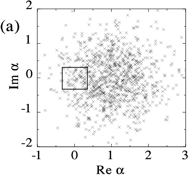
Let us consider balanced double-homodyne detection (Fig. 2) and first assume perfect detection. Each experimental event then gives a pair of real numbers which, after rescaling, define a point in the phase space of the signal, and the probability density of detecting the space points is equal to the $Q$-function of the signal state [11]. When the $j$th measurement yields the phase-space point with polar coordinates $(r_{j},\varphi_{j})$ and altogether $N$ measurements are performed, then the exponential phase moments can be estimated to be

$$\Psi_{k}^{({\rm est})}=\frac{1}{N}\sum_{j=1}^{N}\exp(k\varphi_{j})K_{k}(r_{j}).$$ (22)

FIG. 2.: Double-homodyne scheme [10]. The signal beam is split on a beam splitter BS₁ and the resulting beams are mixed with strong coherent local oscillator (LO) on the beam splitters BS₂ and BS₄. The LO beams at BS₂ and BS₄ stem from a common source, split at BS₃, and their phases differ by $\pi/2$, determined by the $\lambda/4$ phase shifter. The difference of photocurrents measured at the detectors D₁ and D₂ is proportional to $q$ and the photocurrent difference at D₃ and D₄ is proportional to $p$.

In order to answer the question of how close is $\Psi_{k}^{({\rm est})}$ to the actual moment $\Psi_{k}$, we calculate the mean value and dispersion of the estimate (22) over all possible measurement results. Since individual measurement outcomes are independent of each other, we can take advantage of the summation rule for mean values and dispersions of independent quantities. Thus, for the real part of $\Psi_{k}^{(\rm est)}$ we get the mean value

$$E\!\left({\rm Re}\,\Psi_{k}^{(\rm est)}\right)=\frac{1}{N}\sum_{j=1}^{N}E\!\left[\cos(k\varphi_{j})K_{k}(r_{j})\right]$$ (25)

$$\hskip 8.61108pt=\,\frac{1}{N}\sum_{j=1}^{N}\int_{2\pi}\!\!d\varphi_{j}\int_{0}^{\infty}\!\!\!r_{j}dr_{j}\,\cos(k\varphi_{j})K_{k}(r_{j})Q(r_{j},\varphi_{j})$$

$$\hskip 8.61108pt=\,\frac{1}{N}N\ {\rm Re}\,\Psi_{k}={\rm Re}\,\Psi_{k},$$

as it should be, and the dispersion

$$D\!\left({\rm Re}\Psi_{k}^{({\rm est})}\right)=\frac{1}{N^{2}}\sum_{j=1}^{N}D\!\left[\cos(k\varphi_{j})K_{k}(r_{j})\right]$$ (28)

$$\hskip 8.61108pt=\,\frac{1}{N}\Bigg{\{}\int_{2\pi}d\varphi\int_{0}^{\infty}rdr\,\cos^{2}(k\varphi)K_{k}^{2}(r)Q(r,\varphi)$$

$$\hskip 8.61108pt-\left[\int_{2\pi}d\varphi\int_{0}^{\infty}rdr\,\cos(k\varphi)K_{k}(r)Q(r,\varphi)\right]^{2}\Bigg{\}}.$$

Similar expressions hold for the imaginary part of $\Psi_{k}^{(\rm est)}$. Since cos${}^{2}(k\varphi)$ $=$ $1/2$ $+$ cos$(2k\varphi)/2$, after performing the angular integration in the first term on the right-hand side of Eq. (28), the radial part contains the product $Q_{0}(r)K_{k}^{2}(r)$ so that this integral over the divergent kernel can become infinite. Let $n_{0}$ be the number of photons at which the Fock expansion of the state starts. Taking into account Eq. (21), we see that the integrand behaves as $\propto$ $\!r^{2(n_{0}-k)+1}$ for small $r$. Thus, the exponential phase moments $\Psi_{k}$ can be directly sampled from the double-homodyne data, provided that $k$ $\!<$ $\!n_{0}$ $\!+$ $\!1$, because in this case the dispersion of the estimation is bounded. In the opposite case of $k$ $\!\geq$ $\!n_{0}$ $\!+$ $\!1$, the statistical fluctuation diverges so that the exponential phase moments cannot be sampled without a proper regularization of the kernels. Note that for states that contain the vacuum, regularization of the kernels is necessary for all exponential phase moments.

FIG. 3.: Output of simulated double-homodyne detection of a coherent state $|\alpha\rangle$, $\alpha=1$ (a), and enlarged detail of the output around the origin (b).

B Kernel regularization and sampling algorithm

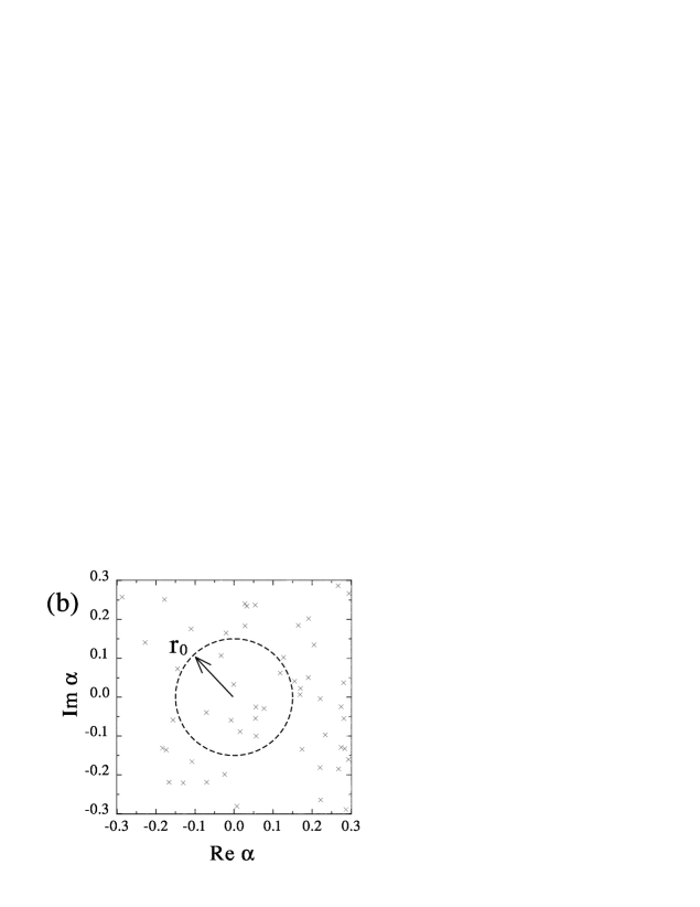
Since the main part of the statistical error arises from data close to the origin, it is natural to modify the procedure by omitting the data falling inside a small circle $r$ $\!<$ $\!r_{0}$ (see Fig. 3). Of course, such a deliberate data filtering introduces into the measurement a state-dependent systematic error. Nevertheless, the statistical error is reduced and the total error may be acceptable. Replacing $K_{k}(r)$ by the regularized function $K^{\prime}_{k}(r)$ according to

$$K^{\prime}_{k}(r)=\theta(r-r_{0})K_{k}(r)$$ (29)

[$\theta(x)$, Heaviside step function], the systematic error of the $k$th moment can be given by

$$\sigma^{(\rm sys)}_{k} = \int_{0}^{2\pi}d\varphi\,e^{ik\varphi}\int_{0}^{r_{0}}rdr\,Q(r,\varphi)K_{k}(r)$$ (30)

$$= \int_{0}^{r_{0}}rdr\,Q_{k}(r)K_{k}(r).$$ (31)

A measure of the total error is then the sum of the statistical and systematic errors,

$${\rm Re}\,\sigma^{(\rm tot)}_{k} = \left|{\rm Re}\,\sigma^{(\rm sys)}_{k}\right|+\left[D\!\left({\rm Re}\ \Psi_{k}^{(\rm est)}\right)\right]^{1/2},$$ (32)

and ${\rm Im}\,\sigma^{(\rm tot)}_{k}$ accordingly.

FIG. 4.: Statistical (a), systematic (b), and total (c) errors of the real part of the sampled exponential phase moment ${\rm Re}\Psi_{2}$ of a coherent state $|\alpha\rangle$, $\alpha$ $\!=$ $\!1$ for different numbers of recorded events $N$.

From the example in Fig. 4 it is seen that the statistical error decreases with increasing radius $r_{0}$ [Fig. 4(a)], whereas the systematic error increases with the radius [Fig. 4(b)]. The total error has thus a minimum at a certain radius [Fig. 4(c)], which can be regarded as the optimal radius for regularization. Unfortunately, the determination of the systematic error requires knowledge of the state. Nevertheless, an upper bound of the systematic error can be estimated, without any a priori knowledge of the measured state. Assuming $r$ $\!<$ $\!1$, we may write

$$\left|Q_{k}(r)\right|=2\sum_{n=0}^{\infty}\frac{r^{2n+k}e^{-r^{2}}}{\sqrt{n!(n+k)!}}\left|\rho_{n+k,n}\right|$$ (35)

$$\hskip 8.61108pt\,\leq 2\,\frac{r^{k}e^{-r^{2}}}{\sqrt{k!}}\sum_{n=0}^{\infty}\sqrt{\rho_{n,n}\,\rho_{n+k,n+k}}$$

$$\hskip 8.61108pt\,\leq 2\,\frac{r^{k}e^{-r^{2}}}{\sqrt{k!}}\sum_{n=0}^{\infty}\frac{\rho_{n,n}+\rho_{n+k,n+k}}{2}\leq 2\,\frac{r^{k}e^{-r^{2}}}{\sqrt{k!}}\,,$$

where we have used the inequality $|\rho_{m,n}|^{2}$ $\!\leq$ $\!\rho_{mm}\rho_{nn}$ implied by positive definiteness of $\rho$. Hence, an upper bound of the systematic error can be estimated. Using Eq. (31), we find that

$$|\sigma^{(\rm sys)}_{k}|\leq\frac{2}{\sqrt{k!}}\int_{0}^{r_{0}}dr\,r^{k+1}e^{-r^{2}}K_{k}(r).$$ (36)

A typical state for which $|\sigma^{(\rm sys)}_{k}|$ is of the order of magnitude of upper-bound value is $|\psi_{k}\rangle$ $\!=$ $\!(|0\rangle$ $\!+$ $\!|k\rangle)/\sqrt{2}$. For this state, $Q_{k}(r)$ $\!=$ $\!r^{k}\exp(-r^{2})/\sqrt{k!}$, which yields one half of the upper bound value. Taking into account that $K_{k}(r)$ $\!\propto$ $\!1/r^{k}$ for $r$ $\!\ll$ $\!1$, we find from the inequality (36) that the upper bound of $|\sigma^{(\rm sys)}_{k}|$ increases quadratically with $r_{0}$. The dependence on $r_{0}$ of the upper bound of the $|\sigma^{(\rm sys)}_{k}|$ is shown in Fig. 5. Notice that the systematic error is smaller for higher $k$.

The state-independent upper bound of the systematic error and the estimated statistical error can now be used to determine the upper bound of the total error. Its minimum then determines an appropriate regularization radius $r_{0}$. A possible algorithm for optimized data processing is the following one. In the zeroth step, sampling of the desired exponential phase moments from all $N$ measurement events is performed. Since also data with very small $r$ may contribute to the result, the statistical error can be very large. In contrast to standard sampling technique, where there is no need for data storage, here the data within a certain small circle are stored. The radius of the circle should be slightly larger than the expected regularization radius. The regularized kernel function (29) is now used, with $r_{0}$ being increased step by step, so that in the $n$th step $n$ events closest to the origin are covered by $r_{0}$. In each step statistical and systematic errors are estimated. The value of $r_{0}$ for which the total error is minimized is used for calculation of the final result.

Let us mention that the detrimental effect of divergent kernels $K_{k}(r)$ at $r$ $\!=$ $\!0$ (in connection with nonzero $Q$-function) resembles the experiment in [10], where the statistics of sine and cosine phases are obtained from low-efficiency double homodyning. In the experiment, data giving rise to divergences are disregarded, which is criticized in [15] from the argument that the disregarded data represent an extra noise in the statistics. In our case, we disregard data leading to high statistical error and include the resulting systematic error into the sampling scheme.

FIG. 5.: Upper bound of $|\sigma^{(\rm sys)}_{k}|$ estimated from the inequality (36) for $k$ $\!=$ $\!1$ (solid line), $k$ $\!=$ $\!2$ (dashed line), $k$ $\!=$ $\!3$ (dot-dashed line), and $k$ $\!=$ $\!4$ (dotted line).

C Total error and number of measurements

Let us assume that a particular phase moment $\Psi_{k}$ is desired to be determined with a prescribed total precision $\sigma^{(\rm tot)}_{k}$. What is the necessary number of measurement events $N$? If there were no need for regularization and the precision were limited only by (finite) statistical fluctuation, then $N$ $\!\propto$ $\!(\sigma^{(\rm tot)}_{k})^{-2}$. When the vacuum contributes to the state to be measured and a regularization radius $r_{0}$ is introduced, then the total error reads

$$\sigma^{(\rm tot)}_{1} = A_{1}(-\ln r_{0})^{1/2}N^{-1/2}+B_{1}r_{0}^{2},$$ (37)

$$\sigma^{(\rm tot)}_{k} = A_{k}r_{0}^{1-k}N^{-1/2}+B_{k}r_{0}^{2},\qquad k\geq 2,$$ (38)

where $A_{k}$ and $B_{k}$ are constants. The optimal regularization radius $r^{\rm(opt)}_{0}$, which minimizes the total error (38) depends on $N$ as

$$r_{0}^{\rm(opt)}\propto N^{-1/[2(1+k)]}\,.$$ (39)

From this expression and Eq. (38) we find that

$$\sigma^{\rm(tot)}\propto N^{-1/(1+k)},$$ (40)

i.e.,

$$N\propto\Big{(}\sigma^{\rm(tot)}_{k}\Big{)}^{-(1+k)}$$ (41)

($k$ $\!\geq$ $\!2$). The case $k$ $\!=$ $\!1$ needs separate consideration, because of the logarithm, which does not provide us with a simple analytical expression. Obviously, $N$ increases faster than ($\sigma^{\rm(tot)}_{1})^{-2}$ with decreasing error. Thus, we can see that in the limit of small total error ordinary homodyning (which does not require regularization) is better suitable for sampling exponential phase moments than the double homodyning, because it requires a smaller amount of data to achieve the same precision.

FIG. 6.: Sampled exponential phase moments of a coherent state $|\alpha\rangle$, $\alpha$ $\!=$ $\!1$; (a) real part of $\Psi_{k}^{\rm(est)}$, (b) imaginary part of $\Psi_{k}^{\rm(est)}$. The error bars indicate the estimated statistical error. In the computer simulation, $N$ $\!=$ $\!10^{6}$ events are recorded and perfect detection is assumed. The dashed regions correspond to the phase moments of the radially integrated $Q$-function.

D Computer simulation

To demonstrate the feasibility of the method, we have performed Monte Carlo simulations of double-homodyne detection of the $Q$-function for sampling the exponential phase moments of a coherent state. Results are shown in Fig. 6 and Table I. From Fig. 6 and Table I it is seen that the sampled exponential phase moments are in good agreement with the exact ones. Note the strong increase of the error with the index $k$ of the moment (for a detailed error analysis, see Fig. 4). Further, a comparison between the dashed and undashed bars in Fig. 6 clearly shows the difference between the concept of canonical phase and the phase concept based on the radially integrated $Q$-function.

In order to compare double homodyning with ordinary homodyning, we have also simulated homodyne detection of the quadrature-component statistics for sampling the exponential phase moments of the same coherent state as in the simulated double-homodyne experiment, using the method in [6, 7, 8]. The results are presented in Table II. Comparing Tables I and II, we see that (for equal total numbers of events) the error in ordinary homodyning is indeed smaller than in double homodyning. The difference between the errors observed in the two schemes increases with increasing index $k$ of the moment. Note that for $k$ $\!=$ $\!4$ the error in the double-homodyne scheme is ten times larger than in the ordinary homodyne measurement.

$k$	$\Psi_{k}$	${\rm Re}\,\Psi_{k}^{(\rm est)}$	${\rm Im}\,\Psi_{k}^{(\rm est)}$	$r_{0}$
1	0.7732	$0.7790\pm 0.0006$	$-0.0008\pm 0.0007~{}~{}$	0.007
2	0.4805	$0.483\pm 0.003$	$0.001\pm 0.003$	0.061
3	0.2559	$0.26\pm 0.01$	$0.00\pm 0.01$	0.160
4	0.1209	$0.13\pm 0.02$	$0.01\pm 0.02$	0.277

TABLE I.: Comparison of the sampled exponential phase moments shown in Fig. 6 with the exact ones. The displayed optimized regularization radii $r_{0}$ refer to Re$\ \Psi_{k}$; values corresponding to Im$\ \Psi_{k}$ are similar in magnitude.

$k$	$\Psi_{k}$	${\rm Re}\,\Psi_{k}^{(\rm est)}$	${\rm Im}\,\Psi_{k}^{(\rm est)}$
1	0.7732	$0.7736\pm 0.0004$	$0.0002\pm 0.0006~{}~{}$
2	0.4805	$0.4795\pm 0.0009$	$-0.0003\pm 0.001$
3	0.2559	$0.2573\pm 0.0017$	$0.0005\pm 0.0017$
4	0.1209	$0.1200\pm 0.0021$	$0.0002\pm 0.0021$

TABLE II.: Comparison of the exponential phase moments of a coherent state $|\alpha\rangle$, $\alpha$ $\!=$ $\!1$, sampled in homodyne detection with the exact ones. In the computer simulation, the $2\pi$-phase interval of the quadrature components is divided into 120 equidistant values, and altogether $N$ $\!=$ $\!10^{6}$ events are recorded.

E Imperfect photodetection

In a real experiment, the overall detection efficiency $\eta$ would be always smaller than $100\%$, but it can be very high, e.g., $\eta$ $\!=$ $\!99\%$. Nonperfect detection introduces additional noise into the sampling scheme and gives rise to an additional systematic error, which cannot be diminished by increasing the number of measurements. The effect of nonperfect detection is that the exponential phase moments of a “smoothed” quantum state are sampled rather than those of the true one. Since the additional noise is Gaussian, the phase-space function that is actually recorded is not the $Q$-function but the function $W_{1-2\eta^{-1}}(q,p)$. The sampling of $\Psi_{k}$ from this function by means of the kernel function $K_{k}(r;-1)$ is equivalent to sampling of $\Psi_{k}$ from the $Q$-function by means of the kernel function $K_{k}[r;-1+2(\eta^{-1}-1)]$. For a given quantum state, the systematic error can thus be given by

$$\Delta_{\eta}\Psi_{k}=\int_{0}^{\infty}\!\!rdr\,Q_{k}(r)\left[K_{k}(r;-1)-K_{k}(r;-3+2\eta^{-1})\right].$$ (42)

Its result is the underestimation of the magnitude of the moment. Since the difference of the kernel functions is essentially nonzero only around the origin $r$ $\!=$ $\!0$, the systematic error $\Delta_{\eta}\Psi_{k}$ will be highest for states close to vacuum. After a proper regularization, one can use Eq. (42) to get a reasonable estimation of the error by substituting the measured statistics for the unknown $Q$-function.

IV Other measurements of the phase-space functions

The phase moments $\Psi_{k}$ can be also obtained from quasidistributions reconstructed in unbalanced homodyning [12], or cavity measurements [16, 17]. However, these methods do not yield $W_{s}(q,p)$ as statistics of events $(q,p)$, but the functions $W_{s}(q,p)$ are determined pointwise. The restriction in practice to a selected finite number of points necessarily results in a systematic error, because the integration over the phase space is replaced by summation over a finite number of points selected by the experimentalist. Having determined $W_{s}(q,p)$, the exponential phase moments $\Psi_{k}$ can then be reconstructed from $W_{s}(q,p)$ on the basis of Eq. (5). Since the kernel function $K_{k}(r;s)$ is well behaved for $s$ $\!>$ $\!-1$, no problems with divergences arise here.

In unbalanced homodyning displaced Fock-state distributions $p(n,\alpha)$ are measured [12, 18]. It can be expected that the cumbersome way of reconstructing $\Psi_{k}$ from $p(n,\alpha)$ via $W_{s}(q,p)$ may be avoided and the reconstruction can be performed directly from the measured data. This could be done in a similar way as in the reconstruction of the density matrix in the Fock basis [19]. A similar approach can be used for different physical systems: statistics of the displaced Fock states of vibrating trap ions has been obtained in state-reconstruction experiments [20], and schemes based on displaced Fock statistics of the cavity fields have been suggested [16, 17]. In particular, the scheme of [16] directly yields the Wigner function, from which the exponential phase moments can be obtained in a very straightforward way. Even though many interesting problems are related to these schemes, we will not deal with them in this paper in any more detail.

V Phase distribution

In order to answer the question of the possibility of direct sampling of the phase distribution itself, we have first to answer the question of the existence of kernels $F(r,\varphi-\psi;s)$ such that

$$P(\varphi)=\int_{0}^{2\pi}d\psi\int_{0}^{\infty}rdr\,W(r,\psi;s)F(r,\varphi-\psi;s).$$ (43)

Obviously, $F(r,\psi-\varphi;s)$ is the ($-s$)-parametrized phase-space function of the phase state $|\varphi\rangle$ in Eq. (2). In [21] it is shown that this function can be given by

$$F(r,\varphi;s)=\sum_{m,n}B_{m,n}(r,s)e^{i(m-n)(\varphi)},$$ (44)

where

$$B_{mn}(r,s)=\sqrt{\frac{n!}{m!}}\,r^{m-n}\left(\frac{s-1}{2}\right)^{n}\left(\frac{2}{1+s}\right)^{m+1}$$ (46)

$$\hskip 51.6665pt\times\,L_{n}^{m-n}\!\left(\frac{4r^{2}}{1-s^{2}}\right)\,\exp\!\left(-\frac{2r^{2}}{1+s}\right)$$

for $m$ $\!\geq$ $\!n$, and $B_{nm}$ $\!=$ $\!B_{mn}$. The series (44) only converges for $s$ $\!>$ $\!0$ (for the limiting case $s$ $\!=$ $\!0$, see also [22]).

FIG. 7.: Plot of the function $F(r,\varphi;0.5)$.

Let us express $F(r,\varphi;s)$ for $s$ $\!>$ $\!0$ in terms of $K(r;s)$. From Eq. (3) it follows that

$$P(\varphi)=\frac{1}{2\pi}\sum_{k=-\infty}^{\infty}\Psi_{k}e^{-ik\varphi}.$$ (47)

Combining Eqs. (47) and (5) and recalling Eq. (43), we may write $F(r,\varphi-\psi;s)$ in the form

$$F(r,\varphi;s)=\frac{1}{2\pi}\left[1+2\sum_{k=1}^{\infty}K_{k}(r;s)\cos(k\varphi)\right].$$ (48)

When $r$ $\!\rightarrow$ $\!\infty$ then $K_{k}(r;s)$ $\!\rightarrow$ $\!1$, and thus $F(r,\varphi,s)$ $\!\rightarrow$ $\!\delta(\varphi)$. Regrouping the terms in Eqs. (A1) and (A2) (for $s$ $\!>$ $\!0$) and using a summation formula for Laguerre polynomials [23], we can rewrite $K_{k}(r;s)$ as

$$K_{k}(r;s)=r^{k}\left(\frac{2}{s\!+\!1}\right)^{k+1}e^{-2r^{2}/(1+s)}$$ (50)

$$\hskip 4.30554pt\times\,\sum_{n=0}^{\infty}\frac{(-1)^{n}}{\sqrt{(n\!+\!1)\ldots(n\!+\!k)}}\left(\frac{1\!-\!s}{1\!+\!s}\right)^{n}L_{n}^{k}\!\left(\frac{4r^{2}}{1\!-\!s^{2}}\right),$$

which is suitable for computing $F(r,\varphi;s)$. An example is displayed in Fig. 7.

The fact that for a large class of states $W(r,\varphi;s)$ does not exist as a regular function for $s$ $\!>$ $\!0$ limits the applicability of Eq. (43). Nevertheless, there exist states for which $W(r,\varphi;s)$ for $s$ $\!>$ $\!0$ is a regular function which can be sampled using unbalanced homodyning. However, for $s$ $\!>$ $\!0$ the statistical error of the sampled $W(r,\varphi;s)$ increases with $r$ [24], so that application of Eq. (43) requires special regularization.

VI Summary and Conclusion

The main results can be summarized as follows. $(i)$ There exist well-behaved kernels for sampling the exponential moments of the canonical phase from $s$-parametrized phase-space functions for $s$ $\!>$ $\!-1$. For $s$ $\!=$ $\!-1$ the kernels diverge in the origin, and for $s$ $\!<$ $\!-1$ the kernels do not exist as regular functions. $(ii)$ Even though for $s$ $\!=$ $\!-1$ the kernels diverge, their integral with the $Q$-function is finite, so that they may be used for inferring the exponential phase moments from the exact $Q$-function. However, the kernel divergence may cause divergent errors of some moments for some states if fluctuating experimental data are used. $(iii)$ Finite errors can be obtained if regularized kernels are used. Since regularization introduces a systematic error, an optimization procedure should be used in order to minimize the sum of the statistical and systematic errors. $(iv)$ The fact that the canonical phase moments can be sampled in double homodyning has an interesting interpretation. Each measurement event yields a unique phase value, but these values must be taken with different weights in dependence on the distance from the origin of the phase space. This is in contrast to the ordinary (four-port) homodyning, where a single measurement does not provide us with a phase value. $(v)$ Even if optimally regularized kernels are used, the amount of data necessary for realizing a desired precision is larger than in standard sampling. This is a disadvantage of the double-homodyne scheme in comparison with ordinary homodyning. $(vi)$ In double homodyning, correct results require perfect detection, because there is no simple possibility of compensation for detection losses, which cause an additional systematic error. This is another disadvantage of double homodyning compared to ordinary homodyning where a compensation of imperfect detection is possible for efficiencies down to $\eta$ $\!>$ $\!0.5$. $(vii)$ Thus, in reply to the question posed in the Introduction, it does not seem that phase-space measurements based on double-homodyning are closer to canonical-phase measurement than quadrature-component measurements based on ordinary homodyning. $(viii)$ In contrast to ordinary homodyning however, the sampling functions in double homodyning are uniquely defined. This follows from the fact that they are actually phase-space representations of quantum mechanical operators. $(ix)$ The exponential phase moments can also be inferred from the data recorded in other schemes such as unbalanced homodyning, in which $s$-parametrized phase-space functions are reconstructed pointwise. $(x)$ Kernels for sampling the distribution of the canonical phase exist as regular functions only for $s$ $>$ 0. Even though for some states the corresponding phase space functions exist and can be measured using unbalanced homodyning, the behavior of the statistical error would require a special regularization of the scheme to be applicable.

A Sampling kernels and the function $\Omega$

Substituting Eq. (9) into Eq. (7) and comparing with Eq. (5), we can express $K_{k}(r;s)$ as

$$K_{k}(r;s)=r^{k}\sum_{l=0}^{\infty}\left(\frac{1-s}{2}\right)^{l}C_{l}^{(k)}L_{l}^{k}\!\left(\frac{2r^{2}}{1-s}\right),$$ (A1)

where the coefficients

$$C_{l}^{(k)}=\sum_{n=0}^{l}\frac{(-1)^{n}}{\sqrt{(n\!+\!1)\dots(n\!+\!k)}}{l\choose n},$$ (A2)

can be rewritten as

$$C_{l}^{(k)}=\frac{1}{\pi^{k/2}}\int_{-\infty}^{\infty}dt_{1}\,e^{-t_{1}^{2}}\ldots\int_{-\infty}^{\infty}dt_{k}\,e^{-kt_{k}^{2}}z_{k}^{l},$$ (A3)

with

$$z_{k}=1-e^{-\rho_{k}^{2}},\qquad\rho_{k}^{2}=\sum_{j=1}^{k}t_{j}^{2}.$$ (A4)

Substituting this expression into Eq. (A1) and using the summation rule

$$\sum_{l=0}^{\infty}\left(\frac{1-s}{2}z_{k}\right)^{l}L_{l}^{k}\!\left(\frac{2r^{2}}{1-s}\right)$$ (A6)

$$\hskip 8.61108pt=\left(1-z_{k}\frac{1-s}{2}\right)^{-k-1}\exp\!\left[\frac{z_{k}r^{2}}{z_{k}(1-s)/2-1}\right],$$

we arrive at

$$K_{k}(r;s)=\frac{r^{k}2^{k+1}}{\pi^{k/2}}\int_{-\infty}^{\infty}dt_{1}\,\bigg{\{}e^{-t_{1}^{2}}\ldots\int_{-\infty}^{\infty}dt_{k}\,e^{-kt_{k}^{2}}$$ (A8)

$$\hskip 4.30554pt\times\left[1\!+\!s\!+\!(1\!-\!s)e^{-\rho_{k}^{2}}\right]^{-\!k\!-\!1}\exp\!\bigg{[}-\frac{2(1\!-\!e^{-\rho_{k}^{2}})r^{2}}{1\!+\!s\!+\!(1\!-\!s)e^{-\rho_{k}^{2}}}\bigg{]}\bigg{\}}$$

Note that the series in Eq. (A6) is only convergent for $|z_{k}(1-s)/2|<1$. We have $z_{k}$ $\!\leq$ $\!1$, thus

$$|(1-s)/2|<1\quad\Rightarrow\quad s>-1$$ (A10)

must hold so that the $Q$-function ($s$ $\!=$ $\!-1)$ represents limiting case for sampling the phase moments.

The multiple integration in Eq. (LABEL:K) can be conveniently performed in hyperspherical coordinates. For this purpose we introduce the function $\Omega^{(k)}(\rho^{2})$ [7],

$$\Omega^{(k)}(\rho^{2})=\int_{0}^{\pi}d\varphi_{1}\,\bigg{[}\sin^{k-2}\varphi_{1}\ldots\int_{0}^{\pi}d\varphi_{i}\,\sin^{k-i-1}\varphi_{i}$$ (A12)

$$\hskip 51.6665pt\times\,\ldots\int_{0}^{2\pi}d\varphi_{k-1}\,\exp\!\bigg{(}-\sum_{l=1}^{k}lt_{l}^{2}\bigg{)}\bigg{]},$$

where

$$t_{i}=\rho\cos\varphi_{i}\prod_{j=1}^{i-1}\sin\varphi_{j}\quad{\rm if}\quad i<k,$$ (A13)

and

$$t_{k}=\rho\prod_{j=1}^{k-1}\sin\varphi_{j},$$ (A14)

with $\rho$ $=$ $\rho_{k}$. The exponent can be expressed in hyperspherical coordinates as

$$\sum_{l=1}^{k}lt_{l}^{k}=\rho^{2}$$ (A16)

$$\hskip 4.30554pt+\,\rho^{2}\sin^{2}\varphi_{1}(1\!+\!\sin^{2}\varphi_{2}(1\!+\!\ldots(1\!+\!\sin^{2}\varphi_{k-1}))).$$

Inserting this expression into Eq. (A12) and expanding the exponential function into a Taylor series, we arrive at Eq. (13) together with Eq. (16). A recurrence formula for the coefficients $A_{n}^{(k)}$ in Eq. (16) can be readily obtained:

$$A_{n}^{(k)}=B_{2n+k-2}\sum_{l=0}^{n}{n\choose l}A_{l}^{(k-1)},\quad k\geq 3$$ (A17)

where

$$B_{j}=\int_{0}^{\pi}d\varphi\,\sin^{j}\varphi=\sqrt{\pi}\frac{\Gamma(\frac{j+1}{2})}{\Gamma(\frac{j+2}{2})},\quad(j\geq 0).$$ (A18)

Starting from $A_{n}^{(2)}$ $\!=$ $\!2B_{2n}$, the formulas (A17) and (13) allow for fast and accurate numerical determination of the functions $\Omega^{(k)}(\rho^{2})$ even for high $k$.

B Asymptotics of $\Omega^{({\rm k})}(\rho^{2})$ and divergence of kernels $K_{\rm k}(r)$

In order to analyze the divergence of the kernels $K_{k}(r)$, we must first know the asymptotic behavior of the functions $\Omega^{(k)}(\rho^{2})$ for large $\rho$. We start from the integral representation (A12) and write the exponent (A16) as

$$\sum_{l=1}^{k}lt_{l}^{k}=\rho^{2}+\rho^{2}\sin^{2}\varphi_{1}\Phi(\varphi_{2},\ldots,\varphi_{k-1}),$$ (B1)

with

$$\Phi(\varphi_{2},\ldots,\varphi_{k-1})=1+\sin^{2}\varphi_{2}(1+\sin^{2}\varphi_{3}(1+\ldots)).$$ (B2)

Note that $\Phi$ $\!\geq$ $\!1$. We insert Eq. (B1) into Eq. (A12) and integrate over $\varphi_{1}$. Assuming $k\geq 2$, the relevant integral is

$$I = \int_{0}^{\pi}d\varphi_{1}\,\sin^{k-2}\varphi_{1}\,e^{-\rho^{2}\Phi\sin^{2}\varphi_{1}}$$ (B3)

$$= 2\int_{0}^{\frac{\pi}{2}}d\varphi_{1}\,\sin^{k-2}\varphi_{1}\,e^{-\rho^{2}\Phi\sin^{2}\varphi_{1}}.$$ (B4)

Assuming $\rho^{2}$ $\!\gg$ $\!1$, we may write $\sin\varphi_{1}$ $\!\approx$ $\!\varphi_{1}$, because the integrand is essentially nonzero only for $\varphi_{1}$ $\!\ll$ $\!1$. From the same argument, we can extend the integration from $(0,\pi/2)$ to $(0,\infty)$,

$$I\approx 2\int_{0}^{\infty}d\varphi_{1}\,\varphi_{1}^{k-2}e^{-\rho^{2}\Phi\varphi_{1}^{2}}=\Gamma\left(\frac{k-1}{2}\right)(\rho^{2}\Phi)^{\frac{1-k}{2}}.$$ (B5)

To finish the calculation of $\Omega$, one has to integrate $\Phi^{(1-k)/2}$ over the remaining angles $\varphi_{2},\ldots,\varphi_{k-1}$ (with appropriate measure). We eventually find the asymptotic behavior

$$\Omega^{(k)}(\rho^{2})\sim C_{k}\rho^{1-k}e^{-\rho^{2}}.$$ (B6)

The factor $\exp(-\rho^{2})$ comes from the first $\rho^{2}$ in Eq. (B1). Taking into account that $\Omega^{(1)}(\rho^{2})$ $\!=$ $\!2\exp(-\rho^{2})$, we see that the asymptotic behavior (B6) holds for all $k\geq 1$.

To investigate the divergence of $K_{k}(r)$ at $r\rightarrow 0$, we make use of the integral representation (LABEL:KERNEL), which is rewritten here as

$$K_{k}(r)=\frac{r^{k}}{\pi^{k/2}}\int_{0}^{\infty}d\rho\,\rho^{k-1}\Omega^{(k)}(\rho^{2})$$ (B8)

$$\hskip 51.6665pt\times\,e^{(k+1)\rho^{2}}\exp\!\left[-(e^{\rho^{2}}-1)r^{2}\right].$$

For small $r$, the dominant contribution to this integral comes from large $\rho$. We can replace $\Omega$ by the asymptotic formula (B6) and absorb the prefactors into $C_{k}$,

$$K_{k}(r)\approx C_{k}r^{k}\int_{0}^{\infty}d\rho\,e^{k\rho^{2}}\exp\!\left[-(e^{\rho^{2}}-1)r^{2}\right].$$ (B9)

Change of the variable according to

$$t=(e^{\rho^{2}}-1)r^{2}$$ (B10)

yields

$$K_{k}(r)\approx\frac{1}{2r^{k}}\int_{0}^{\infty}dt\left(\ln\frac{t+r^{2}}{r^{2}}\right)^{-1/2}(t+r^{2})^{k-1}e^{-t}.$$ (B11)

The integration region of (B11) can be divided in two parts, $t$ $\!<R^{2}$ and $t$ $\!>R^{2}$, with $R$ $\!\approx$ $\!r$. For small $r$, the dominant contribution stems from the latter part where the approximation

$$\ln\frac{t+r^{2}}{r^{2}}\approx\ln\frac{1}{r^{2}}$$ (B12)

can be used, and we find that

$$K_{k}(r)\approx\frac{(-2\ln r)^{-1/2}}{2r^{k}}\int_{0}^{\infty}dt(t+r^{2})^{k-1}e^{-t}.$$ (B13)

The integral is finite for $r$ $\!\rightarrow$ $\!0$, and thus

$$K_{k}(r)\sim\frac{r^{-k}}{(-\ln r)^{1/2}}.$$ (B14)

The logarithm singularity in the denominator is very weak in comparison to the polynomial one in the numerator. Only the polynomial divergence is relevant in Eq. (5), because it determines whether the integral is convergent or not. Thus we need not consider the logarithmic part, so that Eq. (B14) simplifies to

$$K_{k}(r)\sim r^{-k}.$$ (B15)

REFERENCES

- [1] A. Lukš and V. Peřinová, Quantum Opt. 6, 125 (1994); R. Lynch, Phys. Rep. 256, 367 (1995); A. Royer, Phys. Rev. A 53, 70 (1996); R. Tanaś, A. Miranowicz, and Ts. Gantsog, in: Progress in Optics, Vol. XXXV, Ed.: E. Wolf, (Elsevier, Amsterdam, 1996), p. 355; D.T. Pegg and S.M. Barnett, J. Mod. Optics 44, 225 (1997); V. Peřinová, A. Lukš, and J. Peřina, Phase in Optics, World Scientific, Singapore 1998.
- [2] J. Ahn, T.C. Weinacht, and P.H. Bucksbaum, Science 287, 463 (2000).
- [3] G.J. Milburn and S.L. Braunstein, Phys. Rev. A 60, 937 (1999).
- [4] U. Leonhardt, J.A. Vaccaro, B. Böhmer, and H. Paul, Phys. Rev. A 51, 84 (1995).
- [5] A.S. Holevo, Probabilistic and Statistical Aspects of Quantum Theory, North-Holland, Amsterdam (1982); T. Opatrný, J. Phys. A. 27, 7021 (1994); 28, 6961 (1995).
- [6] T. Opatrný, M. Dakna, and D.–G. Welsch, Phys. Rev. A 57, 2129 (1998).
- [7] M. Dakna, T. Opatrný, and D.–G. Welsch, Opt. Commun. 148, 355 (1998).
- [8] M. Dakna, G. Breitenbach, J. Mlynek, T. Opatrný, S. Schiller, and D.–G. Welsch, Opt. Commun. 152, 289 (1998).
- [9] D.–G. Welsch, W. Vogel, and T. Opatrný, in: Progress in Optics, Vol. XXXIX, ed. E. Wolf (Nort-Holland, 1999), p. 63.
- [10] J.W. Noh, A. Fougeres, and L. Mandel, Phys. Rev. Lett. 67, 1426 (1991); Phys. Rev. A 45, 424 (1992); ibid. 46, 2840 (1992).
- [11] M. Freyberger and W. Schleich, Phys. Rev. A 47, R30 (1993); for determining the -function by balanced six-port homodyning, see A. Zucchetti, W. Vogel, and D.–G. Welsch, Phys. Rev. A 54, 856 (1996), M. Paris, A. Chizhov, and O. Steuernagel, Opt. Commun. 134, 117 (1997).
- [12] S. Wallentowitz and W. Vogel, Phys. Rev. A 53, 4528 (1996); K. Banaszek and K. Wódkiewicz, Phys. Rev. Lett. 76, 4344 (1996).
- [13] J. Peřina, Quantum Statistics of Linear and Nonlinear Optical Phenomena, 2nd ed., Kluwer, Dordrecht, 1991.
- [14] G.M. D’Ariano and M.G.A. Paris, Phys. Rev. A 60, 518 (1999).
- [15] Z. Hradil, Phys. Rev. A 47, 4532 (1993).
- [16] L.G. Lutterbach and L. Davidovich, Phys. Rev. Lett. 78, 2547 (1997).
- [17] C.T. Bodendorf, G. Antesberger, M.S. Kim, and H. Walther, Phys. Rev. A 57, 1371 (1998).
- [18] Alternatively, with a fixed can be treated as a generalized phase space function based on scalar product of the signal state with a displaced Fock state. Such a function is another representation of the signal state.
- [19] T. Opatrný and D.–G. Welsch, Phys. Rev. A 55, 1462 (1997); T. Opatrný, D.–G. Welsch, S. Wallentowitz and W. Vogel, J. Mod. Optics 44, 2405 (1997).
- [20] D. Leibfried, D.M. Meekhof, B.E. King, C. Monroe, W.M. Itano, and D.J. Wineland, Phys. Rev. Lett. 77, 4281 (1996).
- [21] J. Eiselt and H. Risken, Phys. Rev. A 43, (1991).
- [22] U. Herzog, H. Paul, and Th. Richter, Physica Scripta T48, 61 (1993).
- [23] A.P. Prudnikov, Yu.A. Brychkov, and O.I. Marichev, Integrals and Series, Gordon and Breach, 1998.
- [24] K. Banaszek and K. Wódkiewicz, J. Mod. Optics 44, 2441 (1997).