Quantum computing with trapped ions, atoms and light

Abstract

We first consider the basic requirements for a quantum computer, arguing for the attractiveness of nuclear spins as information-bearing entities, and light for the coupling which allows quantum gates. We then survey the strengths of and immediate prospects for quantum information processing in ion traps. We discuss decoherence and gate rates in ion traps, comparing methods based on the vibrational motion with a method based on exchange of photons in cavity QED. We then sketch the main features of a quantum computer designed to allow an algorithm needing $10^{6}$ Toffoli gates on 100 logical qubits. We find that around 200 ion traps linked by optical fibres and high-finesse cavities could perform such an algorithm in a week to a month, using components at or near current levels of technology.

1 Introduction

This paper will discuss various issues in the physics of ion traps and quantum information. Our purpose is to address some quite general questions about quantum information physics and ion (or atom) traps, with the aim of identifying useful directions for theoretical and experimental research in the near future and the longer term.

We begin in section 2 by considering the major requirements of a quantum computer without assuming any particular technology from the outset. Rather, we try to identify physical phenomena which appear to be intrinsically well-suited to quantum computing, using arguments based as much as possible on fundamental physical principles. We find that there is a natural link with methods in quantum optics, such as ion and atom trapping and cooling. In section 3 we focus our attention on currently achieved experimental results, considering the particular strengths of ion trap methods. Section 4 briefly surveys the main experiments in quantum information physics which are feasible in the near future using ion traps. These include several fundamental quantum information effects which have not yet been observed in any area of physics. In section 5 we examine how far ion trap methods can go: we estimate the major limitations to the gate rate, at given precision, for two different methods to implement the gates. These are the coupling via the vibrational degree of freedom which has been used up till now, and coupling via cavity quantum electrodynamics (CQED) methods. In section 6 we sketch a design for a moderately large quantum computer: one which could perform $10^{6}$ Toffoli gates on 100 logical qubits. This computer, based on atomic physics and CQED concepts, is conceivable using current technology, and the quantum optics methods it is based on are probably necessary in any case for quantum communication links. It illustrates the power of these methods, and underlines the interest of further experiments, and theoretical studies, in this area.

2 An ideal physical system for quantum computing

We would like to consider the question, what might be the ideal system for a future quantum computer? Here, we do not intend to restrict attention to any one branch of physics (or other science). Rather, we want to know what system we might choose, if we are guided only by basic physical principles and the properties of systems which, in some useful sense, Nature provides.

We would like our ideal quantum computer to have the highest quality memory, logic gates, and read-out. We note that the read-out gives automatically the ability to prepare simple initial states such as product states. By “highest quality” we mean primarily reliable operation, but if the system or the gate can also be small or fast, then so much the better.

For a quantum memory, we want a system of qubits which does not interact with anything else, while for logic gates we want a coupling between qubits which is fast, and not coupled to anything other than the bits. These two demands are almost, but not quite, contradictory. They imply that a quantum computer should be composed of entities $q$ which are, in their passive state when no gates are switched on, almost completely isolated, and yet which can be coupled rapidly. This means they must have a strong coupling to something, $\cal G$. The conflicting demands are met if $\cal G$ has the property that it can be made to be wholly absent when it is not wanted, and introduced rapidly when it is wanted. Furthermore we would like $\cal G$ to interact only with the entities $q$ and with nothing else.

It turns out that Nature does provide a physical entity $q$ which meets the contradictory demands of memory and logic gates better than we might have imagined possible. This entity is the nuclear spin. The advantages of nuclear spins for quantum computing are already well recognised. A spin has a smaller coupling to its environment than any degree of freedom based on charge or the motion of particles; a nuclear spin has a particularly small magnetic moment, and this tiny magnet comes ready-packaged in an electron cloud with highly useful properties for logic gates. The atomic electrons provide the means to take hold of the atom and place it where we wish, and they also provide a ready-made very strong and very stable magnetic field on the nucleus. This results in the hyperfine splitting. The stability of this splitting for isolated atoms or ions is well documented, and is in fact used to provide our standards of time and frequency.

The existence of hyperfine structure makes it possible to couple to the nuclear spin via the electronic state. This provides the handle whereby logic gates can be achieved. The next question is, what is the best way to grasp this handle?

The existing proposals which are based on the nuclear spin and/or hyperfine splitting differ in the way the coupling $\cal G$ is brought about. These proposals include bulk nuclear magnetic resonance (NMR) [1, 2, 3], ion trap [4] and other atomic-physics-based methods [5, 6], and a proposal for future solid state devices based on nuclear spins of dopant atoms implanted in a semiconductor [7].

In bulk liquid-state NMR, the electronic ‘handle’ is almost entirely ignored, and the method relies instead on the tiny direct spin-spin interaction between neighbouring nuclei in a molecule. This permits logic gates but not a direct measurement of the spin state. The fact that all neighbouring qubits are permanently coupled in such methods has both advantages and disadvantages. The other methods all use the electronic ‘handle’. Ion trap experiments up till now have used a light-induced coupling between the electronic state and the vibrational motion (phonon) of relatively heavy charged particles (ions) in a trap in vacuum [4, 8, 9, 10, 11]. There are proposals in which light alone is used to couple the electronic state of one atom and another [5, 12], and a realisation of this concept (in an experiment not based on nuclear spin or hyperfine interaction) using a beam of neutral atoms [13]. The solid state proposal is to use low-mass charged particles (electrons) moving in a solid to provide the coupling [7].

Elaboration on the above summary would enable us to see various strengths and weaknesses of current proposals. However, our purpose here is to seek a method which appears to be in some sense natural, that is, which makes use of physical principles which are naturally suited to the task. We suggest that the natural, and possibly in the long term the best, choice for the entity $\cal G$ which provides rapid controllable coupling, is light. Light is in any case the fundamental coupling between charges. It will travel at the fastest possible speed between qubits, it can be made to appear and disappear at will and, perhaps most importantly, it does not couple to extraneous electromagnetic fields in the computer, which greatly reduces possible decoherence mechanisms. Furthermore, photons provide a natural way to couple quantum information out of the computer and down a quantum communication link.

To ensure there is no light when it is not wanted, we should use frequencies well above the thermal spectrum at the temperature of the computer, but otherwise the main consideration is ease and precision of manipulation of the light (including the ability to select individual qubits). This suggests near-infra-red or optical frequencies. When we wish to couple resonantly to the hyperfine splitting, which is in the microwave domain, we use Raman transitions. Note that the typical frequency scale for hyperfine splitting, i.e. GHz, is attractive because electronic techology allows the most precise control in this frequency regime. This is likely to remain true in the future, owing to basic properties of electromagnetism and conduction in metals.

At this point in the argument, we may envisage an ideal quantum computing system as based on an array of nuclear spins inside atoms, the spins coupling to the electrons of their atoms, and the electrons coupling to photons which ferry information around the computer, appearing and disappearing at the behest of the controlling machinery. The only remaining question is, how is the electron-photon coupling to be both strong enough, and under sufficient control?

To achieve a strong enough coupling, the light must be confined in a small volume, and to permit coherent coupling we require a long photon storage time in the confining cavity, as well as accurate positioning of the atoms. These considerations will be addressed in section 5.

It is possible to imagine that the atoms might be held in place by any one of a number of methods, including attaching them to long chain molecules or fabricating nanoscale structures to hold them. However, the additional atoms and electrons which form the body of any such structures will introduce new degrees of freedom which may cause decoherence, or weaken the light-atom coupling. One possibility is to situate the atoms on the surface, or perhaps under the surface, of a highly transparent solid (see section 6). In this paper we will concentrate on the case that the atoms are held in an r.f. Paul trap (ion trap) or an optical dipole force trap, and consider the possibility of placing the atoms on a surface in the final section.

We note that whereas we have advocated using the nuclear spin alone as quantum memory, current experiments designed to achieve quantum information processing in ion traps are not operating in this regime. In the work of Wineland et al. [8, 9, 10] with the beryllium ion the qubit involves both nuclear and electron spin, since its energy level separation is a sum of hyperfine and first-order Zeeman effects. A pair of electronic states (Coulomb interaction with the nuclear charge) with first order Zeeman effect is adopted in [11, 14, 15] and the electron spin alone in [16]. We envisage that all these experiments will contribute to the overall development of the field, and it will be a relatively small step to adapt them to hyperfine transitions with no electron spin component.

3 Strengths of ion trap technology

Before discussing future prospects, we will highlight in this section the strengths of current ion trap technology.

We consider the three requirements for quantum information processing, which are quantum memory, quantum logic gates, and measurement of quantum states. The primary consideration for all of these is precision and reliability, simply because we need the computer to work; we are willing to sacrifice both speed of operation, and ease of construction, if it makes the difference between a computer which works and one which does not.

Note that all the three requirements are equally significant. In particular, measurement is at the heart of error correction protocols [17, 18], therefore it is a central consideration during the whole operation of the computer, not merely at the final step where the computation result is measured. For some purposes, it is sufficient that a dissipation process can be applied to chosen quantum bits at chosen times [19]. The dissipation process forces the qubit to a known final state, no matter what its initial state. This can be easier to implement, so will be considered also.

3.1 Quantum memory and single-qubit gates

We discussed the attractive features of nuclear spins for quantum computing in section 2. Experiments with trapped atoms and ions offer the most precise methods known for manipulation of the nuclear spin, via the hyperfine interaction. Indeed, time and frequency standards throughout the world are based on optical manipulation of atoms trapped in high vacuum, and ion trap frequency standards now rival those based on neutral atoms. This is the first advantage of ion trap methods. From a practical point of view it means that the quantum memory and single-qubit gates are, broadly speaking, solved problems, in that we can envisage trapped ions whose nuclear spin state is as accurately preserved and manipulated as anything which current technology allows.

3.2 Read-out

The read-out is also, broadly speaking, a solved problem for experiments with trapped atoms or ions. The measurement of the hyperfine state can be carried out rapidly by the electron shelving (or ‘quantum jump’) method, which offers close to 100% reliability [20, 21, 22, 16, 9, 14]. The timescale for such a measurement is set by the need to scatter a few thousand photons on an allowed atomic transition, requiring of order a few hundred $\mu$s. For dissipation, we can use the method of optical pumping. Here, only a few photons need to be scattered before we can be confident the system has relaxed, so the time scale for controlled dissipation is of order $0.1\;\mu$s.

A further point about measurement is significant: as long as separate atoms or ions can be resolved by an optical imaging system (implying a separation of at least a few wavelengths) then they can be measured simultaneously.

The central problem for ion trap quantum computing is, then, the question of implementing the 2- or more-bit logic gates. This will be discussed in section 5.

3.3 Quantifying qubits, gates and entanglement

The standard way to quantify the complexity of an algorithm on any computer, whether quantum or classical, is to count the number of bits in the memory and the number of 2-bit or 3-bit logic gates used. In the case of quantum computing, it makes sense also to have a measure of the degree to which an algorithm involves highly non-classical effects. A useful measure is to ask whether $n$-particle entangled states, such as the “Schrödinger cat” state $\left|{000\cdots 0}\right>+\left|{111\cdots 1}\right>$, can be produced.

So far no ion trap experiment has combined all the necessary features to allow general processing on more than one ion. However, all the ingredients of general processing have been demonstrated in separate experiments[8, 9, 14, 11], and highly entangled states have been produced[9, 10].

The definition of entanglement requires some comment. If two or more separate spin-half particles are in a joint state $\left|{\phi}\right>$, then the existence of a non-zero overlap with an entangled state does not necessarily imply the presence of entanglement. For example, the overlap between the 4-qubit separable state $\left|{++++}\right>$ (where $\left|{+}\right>=(\left|{0}\right>+\left|{1}\right>)/\sqrt{2}$) and the cat state $(\left|{0000}\right>+\left|{1111}\right>)/\sqrt{2}$ is $1/8$. Also, a superposition $\left|{M=+3/2}\right>+\left|{M=-3/2}\right>$ of the two stretched states of a spin-$3/2$ particle is not entangled, even though it could be written $\left|{0}\right>\left|{0}\right>+\left|{1}\right>\left|{1}\right>$ by a suitable choice of state labels. The latter point is important: the mere fact that a state can be written $\left|{0}\right>\left|{0}\right>+\left|{1}\right>\left|{1}\right>$ in some basis is not enough to mean that it is entangled in any sense which is significant to quantum information physics. A strict definition of the term “entanglement” would restrict its use to refer only to degrees of freedom which could in principle be located in separate spatial locations (so that entanglement-enhanced communication could be realised), or which could be used to gain the reduction in computational complexity offered by quantum computation (compared to classical computation) for certain algorithms. In that case the state of spin and motion of an electron emerging from a Stern-Gerlach apparatus would not be regarded as entangled. However, it has become quite common to broaden this strict definition slightly, so as to include the case of “entanglement” between the internal and motional degree of freedom of a single particle.

Such entanglement has been achieved between the internal state of a single trapped ion and its motional state, with a high degree of precision and control, in at least two laboratories [23, 11]. A measure of the degree of entanglement is the size of the Hilbert space in which coherent evolution is demonstrated in the experiment. For example, the “Schrödinger cat” states realised in [23] involve a superposition of coherent states. Each coherent state has a Poissonian distribution over vibrational levels, characterised by a parameter $\alpha$ which had the value $\alpha=2.97\pm 0.06$ in the experiments. The mean vibrational quantum number $\langle n\rangle=|\alpha|^{2}\simeq 9$, and standard deviation $\sigma_{n}\simeq|\alpha|\simeq 3$. The size of the motional Hilbert space in which coherent evolution must take place in order to observe the interference is of order $\log_{2}(\langle n\rangle+1+\sigma_{n})\simeq 3.7$ qubits. Adding the internal degree of freedom, this is a “cat state” of $4.7$ qubits.

A true multi-particle entanglement is very rare in physics, and indeed for more than three particles it has only been achieved, to our knowledge, in a single experiment. This is the 4-particle entanglement recently demonstrated in an ion trap experiment by Sackett et al. [10].

The strength of ion trap experiments which is underlined by this achievement is that the generation of entanglement is under complete experimental control: it is deterministic, rather than being the result of a process which relies on an essentially random event (e.g. spontaneous parametric down-conversion, or velocity selection of atoms from a thermal source). This is a significant distinction because the amount of $n$-qubit entanglement produced by a random process falls off exponentially with the number $n$ of qubits, and therefore results in a system which cannot exhibit some of the essential defining features of quantum computation, such as the breaking of the classical hierarchy of complexity classes.

It is noteworthy that in all experimental “realisations” of quantum algorithms so far reported, the size of the apparatus, or the duration of the experiment, has scaled with the number of qubits required to define the problem at the same rate or worse than a classical computer or information channel would scale with the number of classical bits.

This does not mean that randomly produced entanglement is uninteresting, since it can be used to demonstrate some of the basic principles of quantum mechanics and quantum information. However, one might draw an analogy with the properties of light sources: a thermal source, with a sufficiently narrow filter in front of it, can produce radiation with just as narrow a bandwidth as is available from a laser, but there remains a qualitative, and practically significant, difference between thermal radiation and laser radiation.

For light sources, a useful parameter which emphasizes that bandwidth is not the only consideration is the number of photons per mode. It would be useful to have a comparable measure for entanglement, such as “the number of singlets per 2-qubit Hilbert space” (a singlet being the 2-qubit entangled state $(\left|{01}\right>-\left|{10}\right>)/\sqrt{2}$). The difficulty in forming such a measure is that the Hilbert space size, unlike the modes of a radiation cavity, depends on which parts of the system we choose to focus our attention on. For example, we may consider all the atoms in a thermal beam, or just those selected by a velocity selector. The least ambiguous measure is arguably that implicit in [9]: we define the entangling efficiency $\epsilon$ to be

the probability that, starting from initial conditions of no entanglement, a singlet can be caused to be present in a predetermined Hilbert space at a predetermined time.

The predetermined Hilbert space means we indicate which systems (eg atoms, spins, photons) will contain the singlet, without the need to check by measuring them, and the predetermined time means we decide beforehand at which moment we want the singlet, without reference to the details of the experimental apparatus (thus ruling out statements such as “1 ms after detector D clicks”, if we can’t predict when detector D will click). The purpose of the quantity defined is to enable us to assess rapidly the slow-down to be expected when the same apparatus is used to form 3-particle, 4-particle and higher forms of entanglement.

In parametric down-conversion experiments reported to date [24], $\epsilon$ was of order $10^{-4}$, and in cavity QED experiments using a thermal atomic beam[13], it was $\epsilon\simeq 3\times 10^{-3}$. For thermal ensembles such as those in current liquid state NMR experiments it is zero [25]. A related quantity, the entangling rate (number of successful singlet-generating runs per unit time) was approximately 8000 s^-1 and 2 s^-1 respectively for the down-conversion and CQED experiments.

The first observation of an entangling efficiency of order 1 was in the experiment of Turchette et. al. [9]. The internal state of two trapped beryllium ions was driven to a singlet state with reliability approximately 70% (with entangling rate approximately 30000 s^-1). The recent report of 4-qubit entanglement arose from further work in the same laboratory [10]. These remain the only demonstrations of a high entangling efficiency in any area of physics.

4 Experiments feasible in the short term

We have noted that the main strengths of current ion trap experiments, compared with other quantum information experiments, are that they allow rapid and reliable measurement, and deterministic entanglement. The following list concentrates on experiments which exploit these strengths, identifying goals which are either not realisable at all in other systems, or for which the ion trap may be the system of choice.

A single trapped ion allows the experimental exploration of two important avenues: the vibrational degrees of freedom, and cavity QED [5, 26, 27]. The interest of the vibrational degrees of freedom is illustrated by the Schrödinger cat [23] and environment engineering [28] experiments which further our understanding and control of decoherence.

With 2 ions in the same trap, some standard quantum information ideas can be demonstrated, such as the EPR experiment [29], “dense coding” [30, 31] and a simple “algorithm” such as Grover’s search algorithm [32]. Of these, the EPR experiment is the most significant, since the detector efficiency problem can be avoided [29]; however the close spacing of the ions makes impractical a test involving space-like separated measurement processes. A demonstration of dense coding would be the first time this idea had been implemented without needing post-selection[31], and hence allowing an unambiguous increase in the capacity of the quantum channel to transmit classical information. However since the ‘channel’ involved only covers a distance of some tens of microns in vaccum, it is of no practical use.

With only 2 qubits it is debatable whether the most significant features of Grover’s algorithm can be demonstrated, but the algorithm would provide a useful way of showing that quite general manipulations of a two-ion system had been achieved.

With 3 ions three highly significant experiments could be done. These are “teleportation” [33], entanglement-enhanced communication [34, 35], and quantum error correction [36]. In addition, a thorough (though still very simple) demonstration of Grover’s algorithm would be possible.

Quantum teleportation is significiant not only in the context of quantum communication, but also as an essential ingredient of fault-tolerant quantum processing[18, 37]. A reliable teleportation experiment within a small quantum processor would therefore be a significant development.

The most accessible example of entanglement-enhanced communication is the “Guess my number” protocol [35], in which three parties use shared entanglement and classical communication to learn the answer to a simple mathematical problem. In order to obtain a result which breaks the classical limits on communication, an experiment of overall reliability above 50% is needed.

The simplest example of quantum error correction requires 3 qubits, which are used to protect a single logical qubit against a restricted class of errors [36]. The set of correctable errors could be, for example, phase errors on single bits. The most striking result is obtained, however, if the errors are not merely unitary precession of the qubits themselves, but non-unitary relaxation processes where information leaks away into the environment. For example, optical pumping could be used to cause a relaxation of one qubit, where, after tracing over the environmental degrees of freedom, the qubit has ‘collapsed’ into a mixed state, with density matrix $P_{0}\left|{0}\right>\left<{0}\right|+P_{1}\left|{1}\right>\left<{1}\right|$. After this, the correction network is applied, and it would still recover the exact encoded state in the three qubits. Furthermore, the process of random error followed by correction, could be repeated many times on the same encoded state.

This process is remarkable from several points of view. After it is repeated a few times, the environment would have had a chance to “measure” all the qubits in the processor, thus causing, one would think, a large perturbation to the state, and yet the qubit of information is perfectly preserved. Alternatively, if we drive optical pumping continuously but weakly on all the qubits, then the loss of fidelity of the qubits is linear with time, for small times, while after correction it becomes quadratic with time, therefore allowing the Zeno effect to be implemented in the case of a relaxation process [38, 39, 40, 41].

The 3-qubit quantum error correction has been investigated in an NMR experiment [42]. Some aspects of the expected behaviour were demonstrated, but owing to the limitations of the pseudo-pure state method, a genuine error correction was not available, since the entropy could not be extracted from the system. This is seen most clearly in two aspects of the experiment. First, in encoding from one qubit into three, the signal size fell by a factor 8, and no subsequent error correction can make up for the increased sensitivity to errors in this situation. Secondly, it was not possible to apply correction repetitively.

Note that all the experiments we have listed for three ions rely on the ability to perform not just unitary processing operations, but also strong measurements of one or more chosen qubits. Successful realisation of the “Guess my number” or the repeatable quantum error correction protocols would be landmarks in quantum information science.

Obviously, there are more and more experiments which are possible as the number of qubits increases, even before useful quantum computation becomes possible.

5 Logic gate methods in ion traps

The first general method proposed to implement quantum logic gates between trapped ions was that discovered by Cirac and Zoller [4]. This is based on using the motional degree of freedom to ferry quantum information from one ion to another. All ion trap quantum processing experiments so far have been based on this idea. A significant further insight was provided by Mølmer and Sørensen [43, 44] who showed how to make better use of the motional degree of freedom, and the recent experiments of [10] are based on these further insights.

Another method to couple separate atoms or ions coherently is to use light to ferry the information around, using the proposal of [5] based on concepts in cavity quantum electrodynamics (CQED).

In this section we will compare the two methods—motional and photon-based gates. We assume some familiarity with both methods on the part of the reader. At present the motional methods are easier to achieve experimentally, but the CQED methods allow, in principle, higher gate rates, and also quantum communication between separate ion- or atom-traps.

There is a subtlety regarding the hyperfine interaction and the optical transitions involved in these methods. The electric dipole optical transitions which we will use do not couple directly to the nuclear spin. In the motional coupling, this implies that the change of internal state of the ion must involve the electronic wavefuntion, so it is not purely a nuclear spin rotation. As a result, the relevant hyperfine levels will typically have a first-order Zeeman effect. In the CQED method, 4 states in the ground hyperfine manifold of a single ion are used. In either case, during the action of the gate, the quantum information is stored in electronic not nuclear degrees of freedom. However, the quantum memory can remain a wholly nuclear spin system: we swap quantum information between Zeeman levels $\left|{M_{F}}\right>$ just before and just after each gate, by driving a Raman transition in the internal state of the ions involved in the gate. We assume this transition can be fast compared to the gate operations to be discussed.

5.1 Motional coupling

The Cirac-Zoller method to implement 2-qubit gates such as ‘controlled not’ between separate ions is to couple the internal state of chosen ions to the vibrational degree of freedom, by driving Rabi flopping on a vibrational sideband of the atomic transition. The phenomena which cause the main limitations of this method are relaxation and/or heating, and off-resonant driving of unwanted transitions.

5.1.1 Relaxation

There are two main sources of relaxation in the ion trap. These are the spontaneous decay of excited states of the ion, and the heating or relaxation of the vibrational degree of freedom. To minimise the effects of these, a compromise between fast and slow operation of the processor is needed.

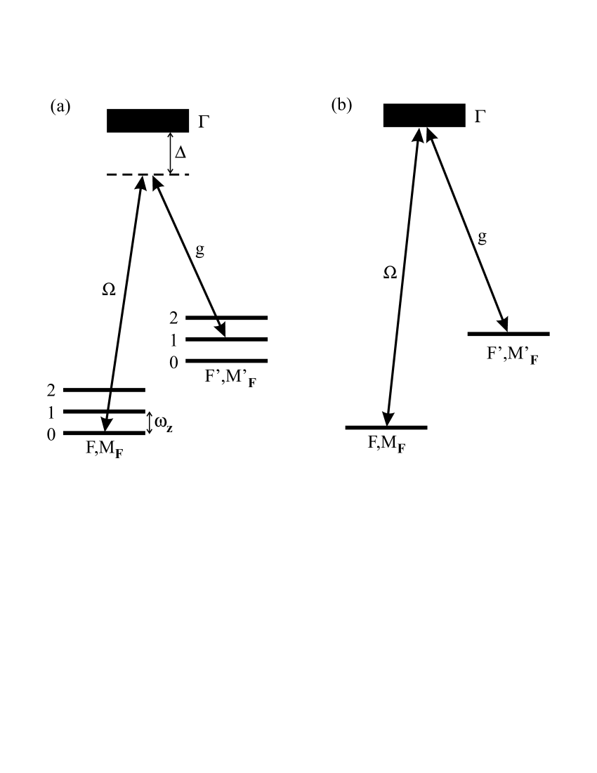
Figure 1: Energy levels and notation for (a) motional gates, (b) CQED optical gates.

The quantum gates between ions involve the excitation of the motional degree of freedom, so we consider driving the first red vibrational sideband of a resonant Raman transition between hyperfine levels in a trapped ion [45], see figure 1. The Raman transition is driven by a pair of lasers detuned by $\Delta\gg\Gamma$ from an allowed single-photon transition whose natural width is $\Gamma$ (full width half maximum in angular frequency units). The Rabi frequencies of the relevant single-photon transitions are $\Omega$ and $g=\eta\Omega$, where $\eta$ is the Lamb-Dicke parameter. In this situation the pair of hyperfine levels connected by the Raman transition form an effective two-level system; the two-level transition has effective Rabi frequency $\Omega_{\rm eff}=\Omega g/2\Delta$. A two-ion gate such as a state-swapping operation requires two $\pi$ pulses on a vibrational sideband, so the total time is $T=2\pi/\Omega_{\rm eff}$. During each pulse the mean population of the unstable excited state of the ion is $\Omega^{2}/4\Delta^{2}$ (assuming $g\ll\Omega$), therefore the mean number of photons scattered is

$$p_{1}=\frac{\Omega^{2}}{4\Delta^{2}}\Gamma T=\frac{\pi\Gamma\Omega}{\Delta g}.$$ (1)

We assume that at all times the vibrational state of the ion suffers a non-unitary heating process, characterised by a rate $\kappa$ which is the rate of heating (or relaxation) from one vibrational state to an orthogonal one. Therefore the probability of relaxation by this process, during the two pulses, is

$$p_{2}=\kappa T=\frac{4\pi\kappa\Delta}{\Omega g}.$$ (2)

The total probability of failure is

$$p=p_{1}+p_{2}=\frac{\pi\Gamma}{g}\frac{\Omega}{\Delta}+\frac{4\pi\kappa}{g}\frac{\Delta}{\Omega}.$$ (3)

In this equation $\Gamma$ is constant for a given atom, and $\kappa$ is characteristic of a given experimental apparatus, while $\Omega/\Delta$ can be adjusted to minimise $p$. This minimisation gives $\Omega/\Delta=2({\kappa}/{\Gamma})^{1/2}$, and

$$p_{\rm min}=4\pi\sqrt{\frac{\kappa\Gamma}{g^{2}}\,},\;\;\;\;\;\;\frac{1}{T}=\frac{g^{2}}{\Gamma}\frac{p_{\rm min}}{8\pi^{2}}.$$ (4)

5.1.2 Off-resonant coupling

The vibrational levels in an ion trap are typically closely spaced compared to all other energy level separations in the system, so the transitions driven off-resonantly are primarily the carrier transitions (those which don’t change the vibrational state), which are off-resonant by the vibrational frequency $\omega_{z}$. This problem is studied in detail in [46]. The conclusion is that after two $\pi$ pulses, the amount of population which leaks into unwanted states due to off-resonant coupling is

$$p_{3}=\frac{\Omega^{2}_{\rm eff,0}}{\omega_{z}^{2}}=\left(\frac{\Omega^{2}}{2\Delta}\right)^{2}\frac{1}{\omega_{z}^{2}}.$$ (5)

where $\Omega_{\rm eff,0}$ is the Rabi frequency for carrier transitions.

5.1.3 Discussion

Of the processes we have considered which limit the motional coupling, the atomic relaxation $\Gamma$ and the off-resonant excitation are intrinsic to the physics of the system, while the motional heating $\kappa$ could in principle be made arbitrarily small (in recent experiments values of $\kappa/\omega_{z}$ as low as $2\times 10^{-7}$ for a single ion [11] and $2\times 10^{-6}$ for the stretch mode of two ions [47] were reported.) Therefore equations (1) and (5) give the main limitations. The gate rate is limited by (5) since for a given value of $\Omega_{\rm eff,0}/\omega_{z}$ we can make $p_{1}\ll p_{3}$ by increasing the laser intensity and its detuning $\Delta$ (until the detuning becomes comparable to further energy-level separations in the ion, such as the fine structure).

In the case that motional heating is significant, the Mølmer-Sørensen approach may be advantageous, since it permits gates of high fidelity in the presence of motional heating (at the expense of reduced gate rate). However, in the limit of small $\kappa$, the gate rate produced by this method in its standard form is limited by off-resonant excitation and is the same as that given in equation (5).

In conclusion, the gate rate at given failure probability $p$ for a 2-qubit swap gate via the motional state is (from (5))

$$\frac{1}{T}=p^{1/2}\eta\frac{\omega_{z}}{2\pi},$$ (6)

assuming $\kappa\ll p/T$ and $\Delta\gg\pi\Gamma/\eta p$, and using either the Cirac-Zoller or the Mølmer-Sørensen methods.

It is notable that this limit, imposed by off-resonant carrier transtions, could be exceeded by exciting the ion in the node of a laser standing wave [4, 48]. That is technically very difficult, but it shows that the physics of the system can allow a faster switching rate. Recently, less demanding methods to gain such a faster rate have been proposed. The Mølmer-Sørensen approach can probably be made to produce faster gates than (6) by a careful choice of parameters [49], and recently a new approach has been put forward in which such a speed up is thoroughly analysed [50]. The latter uses a light-shift-induced resonance, yielding a gate rate $\eta\omega_{z}/2\pi$ and gates of fidelity approximately $1-\eta^{2}/2$. Therefore the speed increase compared to eq. (6) is significant, of order $1/\eta$.

5.2 Photon-based coupling

We will now consider coupling qubits via the excitation of a mode of a high-finesse optical cavity.

We will assume an allowed electric dipole transition, so the Rabi frequency describing the coupling is $g=Ed/\hbar$ where $E$ is the electric field of the light, and $d$ is the electric dipole matrix element. We will use this coupling to exchange quantum information between an atom and a light field by absorption or emission of single photons, therefore we are interested in the value of $g$ when the electric field is that of a single photon. If the photon has angular frequency $\omega$ and occupies a mode of volume $V$, then its energy is $\hbar\omega=\epsilon_{0}E^{2}V/2$, hence

$$g=d\sqrt{\frac{2\omega}{\epsilon_{0}\hbar V}}$$ (7)

The strongest electric dipole matrix elements in atoms are all of order $ea_{0}$ where $e$ is the charge on the electron and $a_{0}$ is the Bohr radius. The spontaneous decay rate $\Gamma$ of an atom on a strong transition varies as $1/\lambda^{3}$:

$$\Gamma=\frac{\omega^{3}d^{2}}{3\pi\epsilon_{0}\hbar c^{3}}$$ (8)

so for $g\gg\Gamma$ the long wavelength region is best. However, we will need the logic gates to be fast, setting a premium on large $g$, hence small wavelengths. The other major source of decoherence is decay of the photon mode owing to the finite finesse of the cavity which contains it. This decay rate is

$$\kappa=\frac{c\pi}{{\cal F}L}$$ (9)

for a cavity of length $L$ and finesse $\cal F$.

5.2.1 Dark state and adiabatic passage

Since we need very precise gates, there is interest in any method to implement them which has reduced sensitivity to the relaxation of the atom and the cavity photon. Such a method is the adiabatic passage, as described in [5]. Briefly, a state-swapping operation is carried out between any two atoms in the cavity by shining laser pulses on the two atoms. The pulses are not exactly simultaneous, but overlap in time, coupling ground states $\left|{a}\right>_{i}$ to each atom’s excited state with Rabi frequencies $\Omega_{i}$, for atoms $i=1,2$ respectively. The cavity mode produces strong coupling between the excited state and a metastable level $\left|{b}\right>_{i}$ simultaneously for both atoms. In our case, $\left|{b}\right>_{i}=\left|{F^{\prime},M^{\prime}_{F}}\right>_{i}$ is in the ground state manifold, separated from $\left|{a}\right>_{i}=\left|{F,M_{F}}\right>_{i}$ by the hyperfine interaction. The system of two atoms plus cavity photon exhibits the phenomenon of dark states, i.e. superpositions of states which by quantum interference are decoupled from the excited states. For up to one photon in the cavity, there are two dark states [5],

$$\left|{D_{0}}\right> = \left|{b,b,0}\right>\equiv\left|{b}\right>_{1}\left|{b}\right>_{2}\left|{0}\right>_{c},$$ (10)

$$\left|{D_{1}}\right> \propto \Omega_{1}g\left|{b,a,0}\right>+\Omega_{2}g\left|{a,b,0}\right>-\Omega_{1}\Omega_{2}\left|{b,b,1}\right>.$$

The swap operation carries one qubit of information from one atom 1 into atom 2. A general operation such as controlled-not is then carried out within atom 2 using four of its states (2 Zeeman components of each of 2 hyperfine levels), then the information is swapped back. Any other atoms in the cavity do not participate because they are not illuminated by the laser pulses, and they are in the states $\left|{a}\right>$ which are not coupled to the cavity photon. To ensure the off-resonant coupling is sufficiently small, we will require the hyperfine splitting to be much larger than $\Omega,\;g$.

The method of adiabatic passage is limited by two considerations. First we need to preserve adiabaticity, and second we need to avoid populating states which suffer non-unitary relaxation. Numerical solution of the master equation for the complete system is discussed in [5]. Here we will make rough estimates in order to identify the best operating regime, for given parameters $g$, $\Gamma$, $\kappa$.

To preserve adiabaticity the rate of change of the conditions must be slow compared to the frequency separation between the state we wish the system to remain in (here, the dark state) and any other state (here, the nearest bright state). For example, if the frequency separation $\omega_{ij}$ and the rate of change of the state are constant in time, then the probability to make an (unwanted) transition from the desired state $\left|{i}\right>$ to some other state $\left|{j}\right>$ after time $t$ is [51]

$$P_{i\rightarrow j}\simeq\left|\frac{dH_{ji}}{dt}\frac{1}{\hbar\omega_{ji}^{2}}\right|^{2}2\left(1-\cos\omega_{ji}t\right).$$ (11)

In our case, we will assume the laser pulses have the form $\Omega_{2}(t)=\{0,\Omega t/T,\Omega\}$ for $\{t\leq 0,0<t<T,t\geq T\}$ respectively, and $\Omega_{1}=\Omega-\Omega_{2}$, therefore $dH_{ji}/dt=\hbar\Omega/T$. The frequency separation between the dark state and the nearest bright state is a complicated function of the Rabi frequencies, which we simplify to $\omega_{ji}(t)\simeq(\Omega_{1}^{2}+\Omega_{2}^{2})^{1/2}$ (it will emerge that for the cavities we will consider, we will need $\Omega\ll g$ in order to minimise the effects of relaxation of the cavity mode). For $P_{i\rightarrow j}\ll 1$ the oscillating term in (11) averages to zero during any interval of time small compared to $T$. We find the probability to make a transition out of the dark state by using the derivative of (11) with respect to time, and then integrating from $t=0$ to $T$, to obtain

$$p_{1}\simeq\frac{4}{T^{2}\Omega^{2}}.$$ (12)

During the adiabatic passage, there is population in the state $\left|{b}\right>_{1}\left|{b}\right>_{2}\left|{1}\right>$ which decays at a rate $\kappa$. We model this by assuming that at any time $t$ the system is in a mixture containing dark state population $1-\int P_{bb1}\kappa dt$, and non-dark state population $\int P_{bb1}\kappa dt$, where $P_{bb1}$ is the population of the $\left|{b}\right>_{1}\left|{b}\right>_{2}\left|{1}\right>$ component in $\left|{D_{1}}\right>$, which, from (10), is approximately $\Omega_{1}^{2}\Omega_{2}^{2}/g^{2}(\Omega_{1}^{2}+\Omega_{2}^{2})$, for $\Omega\ll g$. The non-dark part of this mixture will be strongly coupled to the environment by photon scattering, but the dark part is unaffected by any process involving $\Gamma$. Therefore the net loss of fidelity is given by the integral of $P_{bb1}\kappa$ over the switching time, which is

$$p_{2}\simeq\frac{\Omega^{2}}{2g^{2}}\kappa T.$$ (13)

The net failure probability of the gate is $p=p_{1}+p_{2}$. We choose $T$ to minimise $p$, and then express the gate rate in terms of $p$ and the coupling parameters, obtaining:

$$\frac{1}{T}\simeq\frac{1}{9}\,p^{2}\frac{g^{2}}{\kappa}.$$ (14)

Note that we can obtain a gate of as high fidelity as we wish (against decoherence by the mechanisms we have considered) by slowing down the processor. The laser intensity must be chosen to give $\Omega=g^{2}(p/3)^{3/2}/\kappa$ to meet the conditions of maximum fidelity. We used the approximation $\Omega\ll g$, which will be valid for this choice of $\Omega$ when $g/\kappa\ll(3/p)^{3/2}$.

5.2.2 Rabi flopping

The method of adiabatic passage suffers from the problem that the gate rate given in equation (14) scales as the square of the failure probability, in contrast to the better scaling properties of equations (4) and (6). To avoid this poor scaling, the single-photon mode can be used in a way analogous to that adopted for the vibrational mode in section 5.1: instead of adiabatic passage in a dark state, we drive Rabi flopping on a chosen atom $A$, using a $\pi$ pulse to place a single photon in the cavity mode, and then a similar pulse on another atom $B$ swaps the information from the cavity mode into atom $B$.

The analysis of this process is exactly as in equations (1)-(4) except that now $g$ is the coupling between atom and cavity mode, $\kappa$ is the relaxation rate of the cavity mode, and since the cavity mode only decays (it does not heat), the relaxation probability given in equation (2) is halved, so we replace $\kappa$ by $\kappa/2$ in equations (2)-(4), obtaining

$$p=2\pi\sqrt{\frac{2\kappa\Gamma}{g^{2}}\,},\;\;\;\;\frac{1}{T}=\frac{g^{2}}{\Gamma}\frac{p}{8\pi^{2}}.$$ (15)

The gate rate is now limited by

$$\frac{g^{2}}{\Gamma}=\frac{3c\lambda^{2}}{2\pi V},$$ (16)

where we have used (7) and (8). From general physical principles, the minimum cavity mode volume $V$ might be expected to scale with wavelength as $\lambda^{3}$, which would imply the processor runs faster at shorter wavelengths. In practice the cavity dimensions are also limited by technological considerations.

The state of the art for high finesse Fabry Perot cavities in the optical domain is indicated by [26] (see also [27]). A pair of mirrors of radius of curvature $10$ cm gave a finesse ${\cal F}=4.2\times 10^{5}$ at $\lambda=852$ nm, and was used to form a cavity of length $L=44.6\;\mu{\rm m}$, Gaussian mode waist $w_{0}=20\;\mu{\rm m}$, hence cavity field decay rate $\kappa/(2\pi)=8$ MHz. The mode volume $V=Lw_{0}^{2}$ yields $g/(2\pi)=70$ MHz for coupling to the D₂ line of atomic caesium, linewidth $\Gamma/(2\pi)=5.3$ MHz. Equation (15) then gives $p\simeq 0.8$.

Another important type of optical cavity is provided by the whispering gallery modes of silica microspheres [52, 53]. Mabuchi and Kimble [54] give the theory of coupling between the whispering gallery mode and an atom positioned at or near the surface of the sphere. On the surface of a $50\;\mu{\rm m}$ radius sphere, for example, the coupling to the D₂ line of neutral caesium atoms ($\lambda=852$ nm) is $g/\Gamma\simeq 6$ and for quality factor $Q\simeq 2\times 10^{9}$ which has been reported [55], $g/\kappa\simeq 174$, giving $p\simeq 0.3$.

Combining (9), (16) and (15) we obtain $p=(4\pi^{2}w/\lambda)(3{\cal F})^{-1/2}$, where $w$ is the average diameter of the mode, so that $V=Lw^{2}$. This implies that it will remain very difficult to obtain $p\ll 1$ for a considerable time, since great improvements in finesse will be needed, as well as a reduction in the mirror or sphere radius of curvature (to reduce the mode volume).

5.2.3 Discussion

The advantage of the adiabatic passage method is that it allows precise gates even in the presence of relaxation of both the atomic excited state and the cavity mode. However, it is generally true that adiabatic methods achieve their greater degree of noise tolerance at the expense of processor speed. In the present case, if a cavity of sufficiently low decay rate can be built, then the Rabi flopping method may be preferable in that it will be faster in the limit of small $p$, and may perform better against further considerations, such as driving of off-resonant transitions.

Since the physics of the vibration of an ion string is similar to that of the excitation of a cavity mode, it ought to be possible to apply a method analogous to the Mølmer-Sørensen one [43, 49] to the case of photon coupling. The essential result of the Mølmer Sørensen method is that the sensitivity to relaxation of the degree of freedom providing coupling ($\kappa$) is reduced by a factor $M$, while the gate time gets longer by the factor $M$. Examining (15) we see that in order to halve $p$, we would need to multiply the factor $M$ by four, increasing the gate time by a factor 4. The gate rate thus scales again as $p^{2}$, as it does in the adiabatic passage method.

5.3 Gate time per ion

In the cases both of motional coupling and of photon coupling, the gate rate is reduced when the number of ions $N$ in the trap increases. For the motional coupling, this is partly because the ion string gets heavier and so has a reduced recoil frequency, and partly because if we wish to allow individual ions to be resolved (for single-ion addressing) the trap confinement must be reduced as more ions are added. For the photon coupling, the slow-down arises because the mode volume must be large enough to enclose all the ions, therefore reducing $g$.

We will assume that the ions are in a linear string, or else a rectangular array, each separated from its neighbours by $s=5\lambda$. This means that if individual addressing is achieved by directing separate Gaussian laser beams on each ion, then the cross-talk between ions would be at the level $10^{-4}$ if each beam had a waist $w=s/(\log 100)^{1/2}\simeq 2.3\,\lambda$. Such a beam can be produced by optics of modest numerical aperture. An alternative way to achieve the individual addressing is discussed by Leibfried [56].

The scaling with $N$ of the motional coupling using the Cirac-Zoller method is discussed in [45, 48, 46]. If we require the closest ions in a string to be separated by at least $s=s(\lambda)$, then the gate time increases approximately as $N^{0.93}$. Approximating this as proportional to $N$, and adopting the breathing mode (vibrational frequency $\sqrt{3}$ times that of the centre of mass mode) for the gates, we obtain from equation (6) a gate time per ion which depends only on the failure probability $p$ and properties of the ion such as its mass and recoil frequency. For candidate ions such as beryllium and calcium, this time is of order $2$ and $10\;\mu$s respectively for $p=0.01$, when $s=5\lambda$.

The faster method of [50] produces a gate rate $\eta\omega_{z}/2\pi$ limited through the limit on $\omega_{z}$ imposed by the need to keep ions separated by $s$. We take $N=140$ as an example, which will be useful in section 6. For the 313 nm transition in the beryllium ion the requirement $s=5\lambda$ leads to $\omega_{z}/(2\pi)=418$ kHz, hence $\eta=0.088$ and gate rate 37 kHz. The 397 nm transition in the calcium ion gives $\omega_{z}/(2\pi)=141$ kHz, $\eta=0.056$ and gate rate 8 kHz. Expressed as a gate time per ion, these examples are $0.2$ and $0.9\;\mu$s respectively, with gate failure probabilities of order $p\simeq\eta^{2}/2\simeq 0.004$ and $0.0016$ respectively.

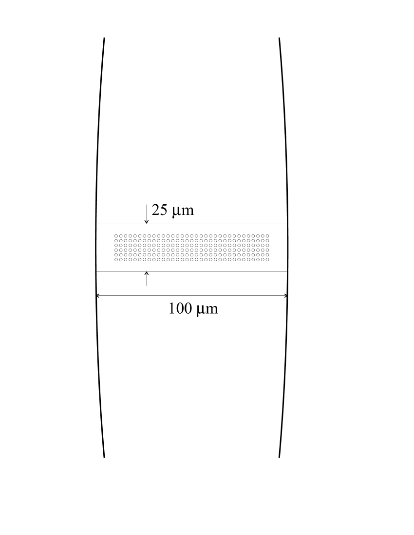
Figure 2: Optical cavity for light-based coupling of 200 qubits, with parameters appropriate to the barium ion. The qubits are shown in a rectangular array spaced by $5\lambda$, which is possible if they are in fact neutral atoms in an optical lattice. In an ion trap they would arrange themselves in another pattern, but the essential features are unchanged (the ions can be made to lie in a plane for a sufficiently elliptical trapping potential).

For photon coupling we take as an example the cavity used in [26] whose properties are summarised in section 5.2.2, with two changes: we reduce the mirror radius of curvature by a fifth (to $2$ cm), and we assume mirrors could be polished to provide the same finesse at half the wavelength. To be precise, we choose $\lambda=493$ nm which is appropriate for the barium ion. This ion can be readily laser cooled, and has the right kind of hyperfine structure for the adiabatic passage approach. The cavity mirrors are placed $L=100\;\mu{\rm m}$ apart, yielding a mode waist $w_{0}=12.5\;\mu{\rm m}$ and $\kappa=(2\pi)3.6$ MHz. The mode can therefore accommodate about 200 ions and equation (14) gives a gate time per ion of $66$ ns for $p=0.01$ (using $\Gamma/(2\pi)=11$ MHz for the $D$ lines in the barium ion, we calculate $g/(2\pi)=62$ MHz). The cavity is illustrated in figure 2.

The conclusion is that for optical cavities which are currently accessible or which may be expected in the near future, the CQED and motional methods have similar speeds (which one is faster will depend on $p$). It would be a lot harder to build the combined optical/atomic system compared to an ion trap alone. However, in principle the optical method could be much faster if suitable cavities could be made, and one possibility for this is a silica microsphere cavity.

6 Design for a quantum computer

In view of the large number of technical problems still to be investigated in the laboratory, it is premature to try to design or build a large quantum computer. However, by sketching the main features of a possible design, we can learn about the issues, and identify avenues for further investigation.

We aim to sketch a design for a quantum computer which could perform algorithms requiring $10^{6}$ Toffoli (controlled-controlled-not) gates on $100$ logical qubits. These numbers are chosen on the basis that about 100 qubits are likely to be needed to allow computations which could not be done on a classical computer. For example, the input to the computation might require 20 qubits, and the further 80 are needed as workspace. A problem needing less than 20 qubits input can probably be solved more easily on a large classical computer. It is important to count Toffoli (or equivalent) gates, not 2-qubit gates such as controlled-not, because Toffoli gates are a major component in any quantum algorithm which cannot be efficiently simulated classically, and, in contrast to controlled-not, it is non-trivial to implement them in a fault-tolerant manner [57, 37]. We take $10^{6}$ gates since Shor’s algorithm requires $O(k^{3})$ gates for a $k$-qubit problem, and a similar scaling is likely to be involved for any useful algorithm.

The computer will rely on fault-tolerant methods and quantum error correction. To be specific, we will adopt the methods described in [18]: the quantum computer consists of blocks of 127 physical qubits, where each block encodes 29 logical qubits in a 7-error-correcting BCH code, and each data block is accompanied by several ancilliary blocks. We place each block in a separate processor, and link processors together by CQED and optical fibre methods [58, 59, 60, 61, 12]. In order to allow low-level error correction methods in addition to those acting at the level of the encoded blocks, each processor will contain 13 extra physical qubits, making 140 in all. These also serve to implement communication protocols between processors, and for other tasks such as probing the local magnetic field.

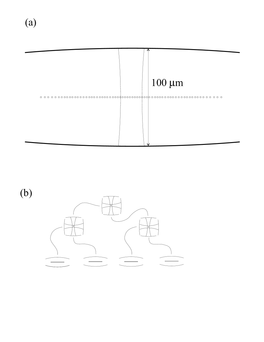
Figure 3: Ion trap and cavity QED-based quantum computer. (a) A single processor consists of 140 calcium ions in a linear trap, with an optical cavity around it. The cavity mirrors are separated by $100\;\mu{\rm m}$ and have radius of curvature 2 cm; the mode waist is $w_{0}=11\;\mu{\rm m}$. Processing within the trap is by motional methods; the optical cavity is used to implement gates between ions in different traps. (b) Processors are connected by optical fibres, and route switching is via small traps with two cavity modes each, coupled into different optical fibres.

We will calculate the processor speed for two designs. The first is a linear ion trap containing calcium ions as described in section 5.3. The gates between ions in a given trap use the vibrational motion, and we adopt the fast gates offered by the lightshift-based concept of Jonathan et al. [50] or by other methods which can be tailored in a similar fashion. To network between processors each ion trap has around it a Fabry-Perot optical cavity, with a mode shape overlapping several ions at the centre of the trap (see figure 3). Note that this cavity should have parameters optimised for quantum communication between traps [58, 59, 60, 61], not for the optical gates discussed in section 5.2. The relevant transitions in calcium have wavelengths around 400 nm. We will also consider a more speculative idea: an all-optical method involving no ion traps. Instead, each processor is a single silica microsphere, with 140 caesium atoms positioned around the circumference of the sphere, either on the silica surface or trapped near it by a dipole force optical trap [54]. The coupling between spheres is by further optical cavities whose design is left unspecified (it is not easy to see how to design them). The characteristics of the sphere are as given in section 5.2.2, except that to accommodate 140 atoms spaced by $5\lambda$ we require a sphere of radius $63\;\mu{\rm m}$ (for this calculation we use the wavelength in silica, since the atoms can be addressed by directing laser beams through the sphere). This reduces $g$ and $\kappa$ by a factor $50/63\simeq 0.8$ from the values quoted in section 5.2.2.

In [18] it was assumed that multiple controlled-not operations, in which there is one control qubit and many target qubits, could be performed in a single time-step. This will not be assumed possible here (but note the comments in [49]), so we must modify the results of [18] accordingly. The preparation of ancillas is slowed down, which will increase the effect of memory noise. In order to reduce this problem, we provide the computer with more ancilla blocks. It can then prepare them in parallel, but staggered in time, so that enough ancillas are always available when they are needed. Providing 40 ancillas per data block (instead of 4 as in [18]) reduces the memory noise requirements by an order of magnitude. The whole computer then needs 138 ion traps and associated optical cavities for the data and ancilla blocks. Further optical cavities, with a few ions in each, may be useful for switching information paths, so that each block can communicate with most other blocks. This brings the total number of ion traps or microspheres and associated cavities to around 200. Using an analysis along the lines of that in [18, 62], we find that the quantum algorithm can be stabilised as long as the failure rate per gate is $\gamma\simeq 10^{-4}$, and the memory noise $\sim 10^{-6}$ per bit per timestep.

To obtain the gate failure probability $10^{-4}$ it is unlikely that the best policy is to use the methods of section 5 alone. Instead, we will assume we can implement a low-level error correction tailored to the physical error process, as for example in [63, 60, 64]. We assume the gates of precision $10^{-4}$ can be built from gates of precision $2\times 10^{-3}$ at a cost of a factor 10 in speed. For the ion trap, the gate time is therefore approximately $10/8000=1250\;\mu$s, using the figures given in section 5.3. The trap would use an axial vibrational frequency of 418 kHz for the centre of mass mode, and frequencies above 20 MHz for radial confinement. Vibrational heating would need to be at the level $\kappa/\omega_{z}<10^{-6}$, which is within current achievements. For the microsphere the gate time is $10\times 35=350\;\mu$s (from (14) with $g=4.8\Gamma=160$ MHz, $\kappa\simeq(g/170)\simeq 0.9$ MHz).

To prepare and verify an ancilla takes $\sim 5000$ time steps [18, 62], but since we prepare ten in parallel for each one we need, the delay before the next one is available is approximately 500 time steps. We envisage that this time is also sufficient to carry out one inter-block controlled-not: that is, 127 controlled-nots at the physical qubit level between ions in separate traps (via the cavities and fibres). Therefore the time per correction of the whole computer is of order $0.2$ to $0.6$ s. We need about 8 such corrections per Toffoli gate in the logical algorithm [18], so the whole algorithm would take two to eight weeks to run.

There are several methods which could be adopted to reduce this run time for the motional gates in the ion trap processor. The trap could be made tighter (increased $\omega_{z}$): the ions at the centre of the string would then be too close to be addressed individually, therefore one would use every other ion in this part of the string. There must be more ions in the trap, which off-sets the speed-up, but overall a factor 2 speed-up is readily obtained, and a higher factor if the spacer ions are of a lighter element. More demanding techniques offer further speed-up, for example by using more than one vibrational mode simultaneously, thus partially parallelizing the gates within a trap. Furthermore, fault-tolerant methods are based on synthesis of highly entangled states [65] and make much use of controlled-multiple-not operations. Such operations can be generated in an ion trap in a time which scales as $N^{1/2}$ rather than $N$ as assumed above [10, 49, 66].

Fabrication of the electrodes for hundreds of ion traps is fairly straightforward, using microfabrication methods or otherwise, as are the low-noise r.f. electronics to provide the trapping fields. For a detailed analysis of experimental issues for processing within each trap we refer the reader to [67, 68] and references therein. Whereas we have not given a thorough treatment of such issues here, we believe the parameters for trap tightness, optical addressing, and heating rates which we have assumed are reasonable. Less well understood is the phenomenon of charge build-up on the optical cavity mirrors, which will influence the operation of an ion trap, and techniques to prevent this may be essential. To build the mirrors for the optical cavities would be a major undertaking, but a possible one. One problem would be slow degradation of the mirrors during assembly or during loading of the traps. To place the mirrors and traps accurately together, and include associated optics such as optical fibres, would be taxing but feasible. The construction and operation of such a quantum computer would have more in common with the construction of a detector in high energy physics than with the manufacture of a classical computer chip; it is a lengthy, expensive and intricate process, but one whose results might merit the investment of resources, if serious uses for a 100-qubit computer can be found. The most important point is that it is conceivable.

In conclusion, ion trap methods currently offer the only way to achieve multi-particle entangled states in a controllable way. They offer the prospect in the fairly near term of achieving various fundamental principles of quantum information physics, such as entanglement-enhanced communication and repeatable quantum error correction. It is clear that the controlled coupling of a trapped ion or neutral atom to a single-photon field in a high-finesse cavity also merits investigation for both quantum communication and quantum computing experiments.

The rough sketch of a quantum computer design which we have given has two significant features: first, it is based on simple physical systems whose behaviour, including decoherence mechanisms, is well understood, and secondly it assumes only currently accessible levels of technology: all the components could be built now. The major unknowns are the detailed experimental issues which may arise when small optical cavities are combined with ion traps, whether the approximate error correction analysis gives a fair estimate of the noise tolerance, and whether suitable low-level error correction protocols, together with high-stability laser systems and magnetic and electric field noise suppression, can provide the $10^{-4}$ gate precision and $10^{-6}$ memory precision required throughout the computer. Further experiments, and more thorough feasibility studies, are certainly called for in this area.

This work was supported by EPSRC, by Christ Church, Oxford and by the European Community network “QUBITS”. We thank D. Stacey for helpful comments on the manuscript.

References

- [1] S. Lloyd, Science 261, 1569 (1993).
- [2] D. G. Cory, A. F. Fahmy, and T. F. Havel, in Proc. 4th Workshop on Physics and Computation (Complex Systems Institute, Boston, MA, 1996).
- [3] N. A. Gershenfeld and I. L. Chuang, Science 275, 350 (1997).
- [4] J. I. Cirac and P. Zoller, Phys. Rev. Lett. 74, 4091 (1995).
- [5] T. Pellizzari, S. A. Gardiner, J. I. Cirac, and P. Zoller, Phys. Rev. Lett. 75, 3788 (1995).
- [6] D. Jaksch, H.-J. Briegel, J. I. Cirac, C. W. Gardiner, and P. Zoller, Phys. Rev. Lett. 82, 1975 (1999).
- [7] B. E. Kane, Nature 393, 133 (1998).
- [8] C. Monroe, D. M. Meekhof, B. E. King, W. M. Itano, and D. J. Wineland, Phys. Rev. Lett. 75, 4714 (1995).
- [9] Q. A. Turchette, C. S. Wood, B. E. King, C. J. Myatt, D. Leibfried, W. M. Itano, C. Monroe, and D. J. Wineland, Phys. Rev. Lett. 81, 3631 (1998).
- [10] C. A. Sackett, D. Kielpinski, B. E. King, C. Langer, V. Meyer, C. J. Myatt, M. Rowe, Q. A. T. amd W. M. Itano, D. J. Wineland, and C. Monroe, Nature 404, 256 (2000).
- [11] C. Roos, T. Zeiger, H. Rohde, H. C. Nägerl, J. Eschner, D. Leibfried, F. Schmidt-Kaler, and R. Blatt, Phys. Rev. Lett. 83, 4713 (1999).
- [12] J. I. Cirac, S. J. van Enk, P. Zoller, H. J. Kimble, and H. Mabuchi, Physica Scripta T76, 223 (1998).
- [13] E. Hagley, X. Maitre, G. Nogues, C. Wunderlich, M. Brune, J. Raimond, and S. Haroche, Phys. Rev. Lett. 79, 1 (1997).
- [14] H. C. Nägerl, D. Leibfried, H. Rohde, G. Thalhammer, J. Eschner, F. Schmidt-Kaler, and R. Blatt, Phys. Rev. A 60, 145 (1999).
- [15] R. J. Hughes et al., Fortschr. Phys. 46, 329 (1998).
- [16] D. Stevens, J. Brochard, and A. Steane, Phys. Rev. A 58, 2750 (1998).
- [17] A. Steane, Rep. Prog. Phys. 61, 117 (1998).
- [18] A. M. Steane, Nature 399, 124 (1999), quant-ph/9809054.
- [19] D. Aharonov and M. Ben-Or, SIAM Journal of Computation , quant-ph/9906129.
- [20] W. Nagourney, J. Sandberg, and H. Dehmelt, Phys. Rev. Lett. 55, 2797 (1986).
- [21] T. Sauter, W. Neuhauser, R. Blatt, and P. E. Toschek, Phys. Rev. Lett. 57, 1696 (1986).
- [22] J. C. Bergquist, R. G. Hulet, W. M. Itano, and D. J. Wineland, Phys. Rev. Lett. 57, 1699 (1986).
- [23] C. Monroe, D. M. Meekhof, B. E. King, and D. J. Wineland, Science 272, 1131 (1996).
- [24] D. Bouwmeester, J.-W. Pan, M. Daniell, H. Weinfurter, and A. Zeilinger, Phys. Rev. Lett. 82, 1345 (1999).
- [25] S. L. Braunstein, C. M. Caves, R. Jozsa, N. Linden, S. Popescu, and R. Schack, Physical Review Letters 83, 1054 (1999).
- [26] J. Ye, D. W. Vernooy, and H. J. Kimble, quant-ph/9908007 (1998).
- [27] P. W. H. Pinkse, T. Fischer, P. Maunz, and G. Rempe, Nature 404, 365 (2000).
- [28] C. J. Myatt, B. E. King, Q. A. Turchette, C. A. Sackett, Kielpinski, W. M. Itano, C. Monroe, and D. J. Wineland, Nature 403, 269 (2000).
- [29] A. Peres, Quantum theory: concepts and methods (Kluwer Academic, Dordrecht, 1993).
- [30] C. H. Bennett and S. J. Wiesner, Phys. Rev. Lett. 69, 2881 (1992).
- [31] K. Mattle, H. Weinfurter, P. G. Kwiat, and A. Zeilinger, Phys. Rev. Lett. 76, 4656 (1996).
- [32] L. K. Grover, Phys. Rev. Lett. 79, 325 (1997).
- [33] C. H. Bennett, G. Brassard, C. Crépeau, R. Jozsa, A. Peres, and W. K. Wooters, Phys. Rev. Lett. 70, 1895 (1993).
- [34] R. Cleve and H. Buhrman, Phys. Rev. A 56, 1201 (1997), quant-ph.
- [35] A. M. Steane and W. van Dam, Physics Today 53, 35 (2000).
- [36] A. M. Steane, Proc. Roy. Soc. Lond. A 452, 2551 (1996).
- [37] D. Gottesman and I. L. Chuang, Nature 402, 390 (1999), quant-ph/9908010.
- [38] L. A. Khalfin, Zh. Eksp. Teor. Fiz. 33, 1371 (1957), and Sov. Phys.—JETP 6, 1053 (1958).
- [39] R. G. Winter, Physical Review 123, 1503 (1961).
- [40] B. Misra and E. C. G. Sudarshan, J. Math. Phys. 18, 756 (1977).
- [41] S. R. Wilkinson, C. F. Bharucha, M. C. Fischer, K. W. Madison, P. R. Morrow, Q. Niu, B. Sundaram, and M. Raizen, Nature 387, 575 (1997).
- [42] R. Laflamme, E. Knill, W. H. Zurek, P. Catasti, and S. V. S. Mariappan, Philosophical Transactions of the Royal Society of London A 356, 1941 (1998).
- [43] K. Mølmer and A. Sørensen, Phys. Rev. Lett. 82, 1835 (1999).
- [44] A. Sørensen and K. Mølmer, Phys. Rev. Lett. 82, 1971 (1999).
- [45] A. M. Steane, Appl. Phys. B 64, 623 (1997).
- [46] A. M. Steane, C. F. Roos, D. Stevens, A. Mundt, D. Leibfried, F. Schmidt-Kaler, and R. Blatt, Phys. Rev. A (2000).
- [47] B. E. King, C. S. Wood, C. J. Myatt, Q. A. Turchette, D. Leibfried, W. M. Itano, C. Monroe, and D. J. Wineland, Phys. Rev. Lett. 81, 1525 (1998).
- [48] D. V. F. James, Applied Physics B 66, 181 (1998), quant-ph/.
- [49] A. Sørensen and K. Mølmer, (2000), quant-ph/0002024.
- [50] D. Jonathan, M. B. Plenio, and P. L. Knight, (2000), quant-ph/0002092.
- [51] Messiah, Quantum Mechanics, volume 2 (PUBLISHER, ADDRESS, YEAR).
- [52] V. B. Braginsky, M. L. Gorodetsky, and V. S. Ilchenko, Physics Letters A 137, 393 (1989).
- [53] V. S. Ilchenko, P. S. Volikov, V. L. Velichansky, F. Treussart, V. Lefèvre-Seguin, J.-M. Raimond, and S. Haroche, Optics Communications 145, 86 (1998).
- [54] H. Mabuchi and H. J. Kimble, Optics Letters 19, 749 (1994).
- [55] L. Collot, V. Lefèvre-Seguin, M. Brune, J.-M. Raimond, and S. Haroche, Europhyics Letters 23, 327 (1993).
- [56] D. Leibfried, Physical Review A 60, R3335 (1999), quant-ph/9812033.
- [57] J. Preskill, Proc. R. Soc. Lond. A 454, 385 (1998), quant-ph.
- [58] J. I. Cirac, P. Zoller, H. J. Kimble, and H. Mabuchi, Phys. Rev. Lett. 78, 3221 (1997).
- [59] T. Pellizzari, quant-ph/9707001 (1997).
- [60] S. J. van Enk, J. I. Cirac, and P. Zoller, Phys. Rev. Lett. 78, 4293 (1997).
- [61] A. Sørensen and K. Mølmer, Physical Review A 58, 2745 (1998).
- [62] A. M. Steane, Fortschritte der Physik (Prog. Phys.) 46, 443 (1997), (preprint quant-ph/9708021).
- [63] J. I. Cirac, T. Pellizzari, and P. Zoller, Science 273, 1207 (1996).
- [64] S. J. van Enk, J. I. Cirac, and P. Zoller, Phys. Rev. Lett. 79, 5178 (1997).
- [65] A. M. Steane, Phys. Rev. Lett. 78, 2252 (1997), quant-ph/9608026.
- [66] J. Steinbach and C. C. Gerry, Physical Review Letters 81, 5528 (1998).
- [67] D. J. Wineland, C. Monroe, W. M. Itano, B. E. King, D. Leibfried, D. M. Meekhof, C. Myatt, and C. Wood, Fortshr. Phys. 46, 363 (1998).
- [68] D. J. Wineland, C. Monroe, W. M. Itano, D. Leibfried, B. E. King, and D. M. Meekhof, J. Res. Natl. Inst. Stand. Technol. 103, 259 (1998).