Self- and cross-phase modulation of ultrashort light pulses in an inertial Kerr medium:
spectral control of squeezed light

Abstract

Quantum theory of self-phase and cross-phase modulation of ultrashort light pulses in the Kerr medium is developed with taking into account the response time of an electronic nonlinearity. The correspondent algebra of time-dependent Bose-operators is elaborated. It is established that the spectral region of the pulse, where the quadrature fluctuations level is lower than the shot-noise one, depends on the value of the nonlinear phase shift, the intensity of another pulse, and the relaxation time of the nonlinearity. It is shown that the frequency of the pulse spectrum at which the suppression of fluctuations is maximum can be controlled by adjusting the other pulse intensity.

Keywords: squeezed light, self-phase modulation, ross-phase modulation, Kerr nonlinearity, ultrashort light pulse.

Received: 23 October 2001,  Accepted: 19 March 2002

1 Introduction

It is well known (see, for example, [1, 2, 3]) that in a nonlinear medium with the Kerr nonlinearity, i.e. with cubic nonlinearity, self-phase modulation (SPM) phenomenon occurs which gives rise to quadrature squeezing of fluctuations with conservation of the photon statistics. This effect is observed when the one-mode radiation propagates in the Kerr medium. If we deal with the propagation of the two-mode radiation in such a medium, the situation becomes more complicated. Besides the SPM effect, the phenomena of cross-phase modulation (XPM) and parametric interactions can, generally speaking, take place. However, the efficiency of parametric frequency-multiplication processes depends on the phase mismatch of the interacting waves. The parametric frequency conversion can be neglected in the case of the strong phase mismatch. It is worthy noting that the influence of the parametric energy exchange at the two-mode interaction on the generation of polarization-squeezed light in the Kerr medium has been considered in [4]. Both SPM and XPM effects do not depend on the phase mismatch, consequently, they can play a dominant role when one investigates the nonlinear propagation of two modes with orthogonal polarizations and/or different frequencies in the Kerr medium. To the best of our knowledge, such analysis has been carried out only for the case of monochromatic modes (see review [5]).

In order to develop a correct quantum theory of the nonlinear propagation of the pulse radiation, it is necessary to take into account a finite response time of the nonlinearity. There are two consistent approaches to solving this problem. In [6, 7] the Kerr nonlinearity has been treated as a Raman -like nonlinearity. The authors [6, 7] have taken into account quantum and thermal noises as a fluctuating addition to the relaxation nonlinearity in the interaction Hamiltonian. In the other approach developed in [8, 9, 10], the interaction Hamiltonian [8] or the interaction momentum operator [9, 10], which contains only a response function of the nonlinearity, have been used. In such quantum description of the SPM of ultra-short pulses (USPs), one cannot add thermal noise terms to the interaction Hamiltonian and momentum operator in order to satisfy the canonical commutation relation for the annihilation and creation Bose-operators.

In this paper, we present the quantum theory based on the interaction momentum operator [9] for the case of nonlinear propagation of two ultrashort light pulses [10]. In reality, here we will mainly analyze two combined (SPM and XPM) effects. The first one is responsible for the generation of the squeezed state of light and the second one (as we demonstrate below) can be employed to control the squeezing process. This combined phenomenon can be shortly called “the SPM-XPM of USPs.” Since we deal with the analysis of the combined phenomena, algebra of time dependent Bose-operators developed earlier in [9, 11] has to be subsequently extended.

The paper is organized as follows.

In section 2 the quantum equations for the SPM-XPM of USPs are introduced when the nonlinearity of medium has relaxation behaviour of an electronic Kerr type. Algebra of time-dependent Bose-operators is extended in section 3 and used to estimate statistical parameters of the USP quadrature components. In section 4 the correlation functions of the quadrature components are obtained. Then in section 5 the spectrum of quadrature-squeezed component of the USP under investigation is studied. Section 6 closes the paper with some concluding remarks.

2 Quantum equations for simultaneous SPM and XPM of light pulses

The conventional way to derive the quantum equation of SPM is based on the interaction Hamiltonian, with the quantum equation describing the time evolution of annihilation or creation Bose-operators being derived. A transition to the space evolution is usually provided by the replacement $t\rightarrow z/u$, where $z$ is the distance passed and $u$ is the pulse’s group velocity in a nonlinear medium. This approach seems to be fairly appropriate for the case of single-mode radiation. Generally speaking, both $t$ and $z$ are present in the analytical description of nonlinear propagation of the pulse. Therefore, the momentum operator connected with the spatial evolution of the pulse field should be used instead of the interaction Hamiltonian [12] in order to obtain an equation for the annihilation Bose-operator. This approach for the case of pulse SPM in nonlinear medium with inertial electronic Kerr nonlinearity has been successfully used in [9].

We start with the analysis of SPM–XPM of two coherent USPs in a noninertial nonlinear medium.

2.1 Quantum SPM-XPM equation in noninertial nonlinear medium

In a noninertial nonlinear medium, the combined SPM–XPM effect of USPs is described by making use of the momentum operator $\hat{G}(z)$ [10]

$$\hat{G}(z)=\sum_{j=1}^{2}\hat{G}^{(j)}_{\rm spm}(z)+\hat{G}_{\rm xpm}(z),$$ (1)

where index $j$ denotes the pulse’s number ($j=1,2$), and the momentum operators of SPM and XPM effects are

$$\hat{G}^{(j)}_{\rm spm}(z) = \hbar\beta_{j}\int_{-\infty}^{\infty}\hat{\mathbf{N}}[\hat{n}^{2}_{j}(t,z)]dt,$$ (2)

$$\hat{G}_{\rm xpm}(z) = \hbar\tilde{\beta}\int_{-\infty}^{\infty}\hat{n}_{1}(t,z)\hat{n}_{2}(t,z)dt.$$ (3)

Here $\hbar$ is Planck’s constant, $\hat{\mathbf{N}}$ is the operator of normal ordering, the factors $\beta_{j}$ and $\tilde{\beta}$ are defined by the electronic Kerr nonlinearity $n_{2}$ of the medium (for example, $\beta_{j}=C^{2}\gamma^{\star}_{j}/2$; $C=(\hbar\omega_{0}/2V)^{1/2}$, $\gamma^{\star}_{j}=k_{0}n_{2{(j)}}/2n_{0}$ [9]), and $\hat{n}_{j}(t,z)=\hat{A}^{+}_{j}(t,z)\hat{A}_{j}(t,z)$ is the photon number “density” operator for the $j$-th pulse in a given cross-section $z$ at the time moment $t$. The operator $\hat{A}^{+}_{j}(t,z)$ [$\hat{A}_{j}(t,z)$] is the photon creation (annihilation) Bose operator. It is the slowly varying operator of the negative (positive) frequency part of the electric field strength operator [13]. The XPM momentum operator defined by (3) takes into account the action of the first pulse on the second one and vice versa.

In the Heisenberg representation, the space evolution for the time-dependent Bose-operator $\hat{A}_{j}(t,z)$ for the $j$-th pulse is given by the equation (see [12])

$$-i\hbar\frac{\partial\hat{A}_{j}(t,z)}{\partial z}=\left[\hat{A}_{j}(t,z),\hat{G}(z)\right].$$ (4)

In accordance with (1), the space evolution equation, for example, of the operator $\hat{A}_{1}(t,z)$ reads

$$\frac{\partial\hat{A}_{1}(t,z)}{\partial z}-\left[i\beta_{1}\hat{n}_{1}(t,z)+i\tilde{\beta}\hat{n}_{2}(t,z)\right]\hat{A}_{1}(t,z)=0.$$ (5)

The spatial evolution equation of the operator $\hat{A}_{2}(t,z)$ can be easily obtained by permuting the indices $1\leftrightarrow 2$. Thus, we get the system of four coupled equations keeping in mind two equations for the creation operator. One points out that Eq. (5) is written in the moving coordinate system: $z=z^{{}^{\prime}}$ and $t=t^{{}^{\prime}}-z/u$, where $t^{{}^{\prime}}$ is the running time, $u$ is the pulse’s group velocity in the nonlinear medium. We assume that one can neglect the difference in group velocities of the pulses and do not consider the pulse spreading due to the medium dispersion, that corresponds to first approximation of the dispersion theory.

In view of Eq. (5), one can show that the operator $\hat{n}_{j}(t,z)$ does not change in the nonlinear medium:

$$\hat{n}_{j}(t,z)=\hat{n}_{j}(t,z=0)=\hat{n}_{0,j}(t),$$ (6)

where $z=0$ corresponds to the input of the nonlinear medium. Equation (6) means that the photon statistics does not change in the medium.

Solving Eq. (5) and its Hermitian conjugate, one has for the annihilation and creation photon Bose-operators

$$\hat{A}_{1}(t,z) = e^{i\gamma_{1}\hat{n}_{0,1}(t)+i\tilde{\gamma}\hat{n}_{0,2}(t)}\,\hat{A}_{0,1}(t),$$ (7)

$$\hat{A}^{+}_{1}(t,z) = \hat{A}^{+}_{0,1}(t)\,e^{-i\gamma_{1}\hat{n}_{0,1}(t)-i\tilde{\gamma}\hat{n}_{0,2}(t)},$$ (8)

where $\gamma_{1}=\beta_{1}z$ and $\tilde{\gamma}=\tilde{\beta}z$. By permuting the indices $1\leftrightarrow 2$, one gets the Bose-operators for another light pulse.

The preservation of the canonical structure of quantum theory requires that the annihilation and creation Bose operators $\hat{A}_{j}(t,z)$ and $\hat{A}^{+}_{j}(t,z)$ satisfy the commutation relations

$$\left[\hat{A}_{j}(t_{1},z),\hat{A}^{+}_{k}(t_{2},z)\right]=\delta_{jk}\,\delta(t_{2}-t_{1})$$ (9)

for an arbitrary distance $z$ in the medium, where $\delta_{jk}$ is the Kroneker delta-symbol, $j,k=1,2$.

There are some peculiarities in the quantum description of the combined SPM–XPM effect in a noninertial nonlinear medium. Firstly, the solutions (7), (8) do not permit to verify the commutation relation (9). Secondly, the reduction of the expressions $e^{i\gamma_{j}\hat{n}_{0,j}(t)}$, $e^{i\tilde{\gamma}\hat{n}_{0,j}(t)}$ to the normally-ordered form is accompanied by the appearance of a nonintegrable singularity (see [9, 11]). These circumstances do not appear in the quantum theory of combined SPM-XPM effect which takes into account the relaxation behaviour of the nonlinearity.

2.2 Quantum equation of pulse SPM-XPM in inertial nonlinear medium

The momentum operator for SPM of USP in a medium with the electronic Kerr nonlinearity has been introduced in [9]. It incorporates the function of a nonlinear response in its structure. In the model considered, a contribution of the electronic Kerr nonlinearity decreases exponentially. Thus, we rewrite the momentum operator of SPM–XPM effect $\hat{G}(z)$ introduced according to (1) (see [10]) as follows

$$\hat{G}^{(j)}_{\rm{spm}}(z)=\hbar\beta_{j}\int_{-\infty}^{\infty}dt\int_{-\infty}^{t}H(t-t_{1})\hat{\mathbf{N}}\bigl{[}\hat{n}_{j}(t,z)\hat{n}_{j}(t_{1},z)\bigl{]}dt_{1},$$ (10)

$$\hat{G}_{\rm{xpm}}(z)=\hbar\tilde{\beta}\int_{-\infty}^{\infty}dt\int_{-\infty}^{t}H(t-t_{1})\bigl{[}\hat{n}_{1}(t,z)\hat{n}_{2}(t_{1},z)+\hat{n}_{1}(t_{1},z)\hat{n}_{2}(t,z)\bigl{]}\,dt_{1},$$ (11)

where $H(t)$ is the function of nonlinear response, asymmetrically defined in order to satisfy the condition imposed by the causality principle: $H(t)\neq 0$ at $t\geq 0$ and $H(t)=0$ at $t<0$. The term in the second integral in (10) should be interpreted as a generalized force acting in the cross-section $z$ of the medium which at the time moment $t$ depends only on the previous time moments. The similar term in the second integral in (11) should be interpreted as a sum of two generalized forces acting between pulses in the same cross-section $z$ of a medium which also depend on the previous time moments. Therefore, the causality principle in the Hermitian operators (10) and (11) is not violated.

In the case of the nonlinearity of an electronic origin, the nonlinear response function can be introduced as follows:

$$H(t)=(1/\tau_{r})\exp{\left(-t/\tau_{r}\right)},\qquad(t\geq 0)$$ (12)

and $H(t)=0$ at $t<0$. Indeed, if a single USP propagates through the Kerr medium, then the evolution of nonlinear addition $\Delta n_{nl}$ to the refractive index, which is associated with the SPM effect, is given by the equation (see, for example, [9, 11, 13])

$$\tau_{r}\frac{\partial\Delta\hat{n}_{nl}(t,z)}{\partial t}+\Delta\hat{n}_{nl}(t,z)=\frac{1}{2}\,n_{2{(j)}}\,\hat{n}_{j}(t,z),$$ (13)

which has the solution

$$\Delta\hat{n}_{nl}(t,z)=\frac{1}{2}\,n_{2{(j)}}\int_{-\infty}^{t}H(t-t_{1})\hat{n}_{j}(t_{1},z)dt_{1}.$$ (14)

Note that the nonlinear response function (12) appears in the absence of one- and two-photon and Raman resonances  [13]. Therefore, the approach developed is valid when each pulse frequency is off-resonance and the pulse duration $\tau_{p}$ is much larger than the relaxation time $\tau_{r}$. If the USP propagates in a fused silica-fiber, then about $80$% of the Kerr effect is due to the electronic motion occurring on $\sim 1$ fs time scales and only $20$% of the Kerr effect is attributable to the Raman oscillators [14]. Thus, our model corresponds to the case of the Kerr effect mainly produced by the electronic motion.

Since in quantum theory the relaxation behaviour is connected with the so-called thermal reservoir, the operator evolution equation (13) must, in general case, contain a source of thermal noise besides a relaxation term. Then we can write the following expression for the nonlinear addition [6, 7]

$$\Delta\hat{n}_{nl}(t,z)=\frac{1}{2}\,n_{2{(j)}}\int_{-\infty}^{t}H(t-t_{1})\hat{n}_{j}(t_{1},z)dt_{1}\,+\,\hat{m}(t,z),$$ (15)

where the Hermitian operator $\hat{m}(t,z)$ takes into account thermal fluctuations of $\Delta\hat{n}_{nl}(t,z)$ in the absence of light field. For the nonlinearity of electronic origin an expression likes (15) can be obtained from Duffing-type equation [13]. Here it is important to note that the average value of $\hat{m}(t,z)$ operator is equal to zero; $\langle\hat{m}(t,z)\rangle=0$ (see also [7]). Hence, one can consider Eq. (14) as the result of averaging Eq. (15) over the thermal fluctuations. In connection with that, expressions (10), (11) can be truly considered as ones averaged over the thermal fluctuations of nonlinearity.

In the present paper we neglect the thermal fluctuations since we are interested in the nonlinear phase fluctuations caused by the quantum USP ones. Nevertheless, the commutation relations (9) are proved to be valued in this simplified approach (see below). However, it is not difficult to generalize the theory of the SPM and XPM phenomena allowing for thermal noise in the Kerr medium with electronic nonlinearity.

Using (9) it is easy to prove that the operator $\hat{n}_{j}(t,z)$ commutes with the the momentum operator $\hat{G}(z)$,

$$[\hat{G}(z),\hat{n}_{j}(t,z)]=[\hat{G}(z),\hat{n}_{0,j}(t)]=0,$$ (16)

that is, the photon number operator $\hat{n}_{j}(t,z)$ remains unchanged in the nonlinear medium [see also Eq. (6)].

Taking into account (10) and (11), one obtains from (4) the quantum equation for combined SPM–XPM effect, for instance, for the pulse with index $1$

$$\frac{\partial\hat{A}_{1}(t,z)}{\partial z}-\left\{i\beta_{1}q[\hat{n}_{0,1}(t)]+i\tilde{\beta}q[\hat{n}_{0,2}(t)]\right\}\hat{A}_{1}(t,z)=0,$$ (17)

where

$$q[\hat{n}_{0,j}(t)]=\int_{0}^{\infty}H(t_{1})\left[\hat{n}_{0,j}(t-t_{1})+\hat{n}_{0,j}(t+t_{1})\right]dt_{1}.$$ (18)

The appearance of the second term in (18) related to $\hat{n}_{0,j}(t+t_{1})$ in the quantum description has been already discussed in [9] where it has been assumed that this term can be connected with the vacuum fluctuations which are present even in the absence of a pulse. It should be also pointed out that expression (17) is an intermediate result written in the moving coordinate system.

Solving the space evolution equation (17) for the annihilation Bose-operator and its Hermitian conjugate we obtain

$$\hat{A}_{1}(t,z) = e^{i\gamma_{1}q[\hat{n}_{0,1}(t)]+i\tilde{\gamma}q[\hat{n}_{0,2}(t)]}\,\hat{A}_{0,1}(t),$$ (19)

$$\hat{A}^{+}_{1}(t,z) = \hat{A}^{+}_{0,1}(t)\,e^{-i\gamma_{1}q[\hat{n}_{0,1}(t)]-i\tilde{\gamma}q[\hat{n}_{0,2}(t)]}.$$ (20)

One can obtain similar expressions for the Bose-operators of the second pulse by permuting indices $1\leftrightarrow 2$. It is convenient to rewrite expression (18) as follows

$$q[\hat{n}_{0,j}(t)]=\int_{-\infty}^{\infty}h(t_{1})\hat{n}_{0,j}(t-t_{1})dt_{1},\qquad[h(t)=H(\left|t\right|)].$$ (21)

If we consider $\hat{n}_{0,j}$ to be time independent, then (19) and (20) describe the case of monochromatic modes (see, for example, [5, 15]). If in (19) and (20) the response function $H(t)=\delta(t)$, then the description of the noninertial nonlinear media (7) and (8) can be produced. Note that in the quantum description the structure of the nonlinear response (21) is similar to the one of a linear response of a medium in second-order approximation of the dispersion theory (see [9, 13]).

To estimate the statistical characteristics of pulses at the output of the nonlinear medium, we need to calculate the average values of the operators’ moments. As it is well known, they can be found if the operator expressions are given in the normally ordered form. The use of solutions (19) and (20) involves the development of a special mathematical technique. Bellow some elements of algebra of time-dependent Bose-operators developed in [9] are extended.

3 Algebra of time-dependent Bose-operators

For the quantum analysis of the pulse’s SPM the correspondent algebra of time-dependent Bose-operators has been developed in [9]. In the case where the XPM effect is present in addition to the SPM effect, we need to improve the mentioned algebra. It is convenient to introduce the operators

$$\hat{O}_{j}(t)=i\gamma_{j}\,q[\hat{n}_{0,j}(t)],\qquad\hat{\tilde{O}}_{j}(t)=i\tilde{\gamma}q[\hat{n}_{0,j}(t)],$$ (22)

and their Hermitian conjugates

$$\hat{O}^{+}_{j}(t)=-\hat{O}_{j}(t),\qquad\hat{\tilde{O}}^{+}_{j}(t)=-\hat{\tilde{O}}_{j}(t),$$ (23)

in order to simplify further calculations. Thus, Eqs. (19), (20) may be represented in the operator form:

$$\hat{A}_{1}(t,z) = e^{\hat{O}_{1}(t)+\hat{\tilde{O}}_{2}(t)}\,\hat{A}_{0,1}(t),$$ (24)

$$\hat{A}^{+}_{1}(t,z) = \hat{A}^{+}_{0,1}(t)\,e^{\hat{O}^{+}_{1}(t)+\hat{\tilde{O}}^{+}_{2}(t)},$$ (25)

where the operator $\hat{O}_{1}(t)$ is responsible for the SPM of the $j$-th pulse and the operator $\hat{\tilde{O}}_{2}(t)$ corresponds to the XPM effect due to the action of the second (control) pulse on the first pulse (under investigation).

We suppose that the initial pulses are in coherent states, the $j$-th pulse’s operator $\hat{A}_{0,j}(t)$ acting only on the state vector $|\alpha_{0,j}(t)\rangle$ within the associated Hilbert space ${\mathcal{H}_{j}}$:

$$\hat{A}_{0,j}(t)|\alpha_{0,j}(t)\rangle=\alpha_{0,j}(t)|\alpha_{0,j}(t)\rangle,$$

where $\alpha_{0,j}(t)$ is the eigenvalue of the operator. The factorization of the states of two different sub-Hilbert spaces ${\mathcal{H}_{1}}$ and ${\mathcal{H}_{2}}$ takes place. The summarized quantum state of two pulses is described by the vector

$$|\alpha_{0}(t)\rangle=|\alpha_{0,1}(t)\rangle\otimes|\alpha_{0,2}(t)\rangle$$

in the global Hilbert space ${\mathcal{H}}={\mathcal{H}_{1}}\otimes{\mathcal{H}_{2}}$. Since the coherent quantum states of each pulse occupy a distinct sub-Hilbert space for any two arbitrary chosen time moments $t_{1}$ and $t_{2}$ one can write :

$$[\hat{n}_{1}(t_{1},z),\hat{n}_{2}(t_{2},z)]=[\hat{n}_{0,1}(t_{1}),\hat{n}_{0,2}(t_{2})]=0,$$ (26)

from which we obtain

$$\bigl{[}\hat{A}_{0,1}(t_{1}),e^{\hat{O}_{2}(t_{2})}\bigl{]}=0, \bigl{[}\hat{A}_{0,2}(t_{1}),e^{\hat{O}_{1}(t_{2})}\bigl{]}=0,$$ (27)

$$\bigl{[}\hat{A}^{+}_{0,1}(t_{1}),e^{\hat{O}_{2}(t_{2})}\bigl{]}=0, \bigl{[}\hat{A}^{+}_{0,2}(t_{1}),e^{\hat{O}_{1}(t_{2})}\bigl{]}=0.$$ (28)

Calculating (27) and (28) it is easy to prove that the following relationships take place:

$$\bigl{[}e^{\hat{O}_{1}(t_{1})},e^{\hat{O}_{2}(t_{2})}\bigl{]} = \bigl{[}e^{\hat{O}^{+}_{1}(t_{1})},e^{\hat{O}^{+}_{2}(t_{2})}\bigl{]}=0,$$ (29)

$$\bigl{[}e^{\hat{\tilde{O}}_{1}(t_{1})},e^{\hat{\tilde{O}}_{2}(t_{2})}\bigl{]} = \bigl{[}e^{\hat{\tilde{O}}^{+}_{1}(t_{1})},e^{\hat{\tilde{O}}^{+}_{2}(t_{2})}\bigl{]}=0.$$ (30)

It should be pointed out that in the next sections the averaging operations are made over the total quantum state $|\alpha_{0}(t)\rangle$.

3.1 Operator permutation relations

For each pulse, the following operator permutation relations hold (see also [9]):

$$\hat{A}_{0,j}(t_{1})\hat{O}_{j}(t_{2}) = [\hat{O}_{j}(t_{2})+{\mathcal{D}}_{j}(t_{2}-t_{1})]\hat{A}_{0,j}(t_{1}),$$ (31)

$$\hat{O}_{j}(t_{1})\hat{A}^{+}_{0,j}(t_{2}) = \hat{A}^{+}_{0,j}(t_{2})[\hat{O}_{j}(t_{1})+{\mathcal{D}}_{j}(t_{2}-t_{1})],$$ (32)

where

$${\mathcal{D}}_{j}(t_{2}-t_{1})=i\gamma_{j}\,h(t_{2}-t_{1}).$$

Besides, $\mathcal{D}_{j}(t_{2}-t_{1})=\mathcal{D}_{j}(t_{1}-t_{2})$ since $h(t)$ is an even function of $t$ [see (21)]. In view of the mathematical induction, it is possible to demonstrate the validity of the formulae ($m\in{\mathrm{N}}$):

$$\hat{A}_{0,j}(t_{1})\hat{O}^{m}_{j}(t_{2}) = [\hat{O}_{j}(t_{2})+{\mathcal{D}}_{j}(t_{2}-t_{1})]^{m}\hat{A}_{0,j}(t_{1}),$$ (33)

$$\hat{O}^{m}_{j}(t_{1})\hat{A}^{+}_{0,j}(t_{2}) = \hat{A}^{+}_{0,j}(t_{2})[\hat{O}_{j}(t_{1})+{\mathcal{D}}_{j}(t_{2}-t_{1})]^{m}.$$ (34)

Expanding $e^{\hat{O}_{j}(t)}$ and $e^{\hat{O}^{+}_{j}(t)}$ in Taylor series, we can get the operator permutation relations which play an important role while estimating the statistical characteristics of the pulse investigated. By using (33) and (34) we finally arrive at

$$\hat{A}_{0,j}(t_{1})e^{\hat{O}_{j}(t_{2})} = e^{\hat{O}_{j}(t_{2})+{\mathcal{D}}_{j}(t_{2}-t_{1})}\hat{A}_{0,j}(t_{1}),$$ (35)

$$e^{\hat{O}_{j}(t_{1})}\hat{A}^{+}_{0,j}(t_{2}) = \hat{A}^{+}_{0,j}(t_{2})e^{\hat{O}_{j}(t_{1})+{\mathcal{D}}_{j}(t_{2}-t_{1})}.$$ (36)

Other permutation relations can be obtained by Hermitian conjugation. Making use of the relations (35), (36) and Eqs. (29), (30) one can show that the canonical commutation relation (9) for the operators $\hat{A}_{j}(t,z)$ and $\hat{A}^{+}_{j}(t,z)$ is exactly fulfilled. Proceeding in the same manner we can prove the validity of the following relations

$$\bigl{[}\hat{A}_{j}(t_{1},z),\hat{A}_{j}(t_{2},z)\bigl{]} = 0,$$ (37)

$${}\bigl{[}\hat{n}_{j}(t_{1},z),\,\hat{n}_{j}(t_{2},z)\bigl{]} = 0.$$ (38)

Let j=1. Then

$$\bigl{[}\hat{A}_{1}(t_{1},z),\hat{A}_{1}(t_{2},z)\bigl{]} = \hat{A}_{1}(t_{1},z)\hat{A}_{1}(t_{2},z)-\hat{A}_{1}(t_{2},z)\hat{A}_{1}(t_{1},z)$$ (39)

$$= e^{\hat{O}_{1}(t_{1})+\hat{\tilde{O}}_{2}(t_{1})}\hat{A}_{0,1}(t_{1})e^{\hat{O}_{1}(t_{2})+\hat{\tilde{O}}_{2}(t_{2})}\hat{A}_{0,1}(t_{2})$$

$$-e^{\hat{O}_{1}(t_{2})+\hat{\tilde{O}}_{2}(t_{2})}\hat{A}_{0,1}(t_{2})e^{\hat{O}_{1}(t_{1})+\hat{\tilde{O}}_{2}(t_{1})}\hat{A}_{0,1}(t_{1})$$

$$= e^{\hat{O}_{1}(t_{1})+\hat{O}_{1}(t_{2})+\hat{\tilde{O}}_{2}(t_{1})+\hat{\tilde{O}}_{2}(t_{2})}e^{\mathcal{D}_{1}(t_{2}-t_{1})}\hat{A}_{0,1}(t_{1})\hat{A}_{0,1}(t_{2})$$

$$-e^{\hat{O}_{1}(t_{1})+\hat{O}_{1}(t_{2})+\hat{\tilde{O}}_{2}(t_{1})+\hat{\tilde{O}}_{2}(t_{2})}e^{\mathcal{D}_{1}(t_{1}-t_{2})}\hat{A}_{0,1}(t_{1})\hat{A}_{0,1}(t_{2})$$

$$= 0.$$

We used above the permutation relation (35). Let us verify our initial statement (6).

$$\hat{n}_{1}(t,z) = \hat{A}^{+}_{1}(t,z)\hat{A}_{1}(t,z)$$ (40)

$$= \hat{A}^{+}_{0,1}(t)e^{\hat{O}^{+}_{1}(t)+\hat{\tilde{O}}^{+}_{2}(t)}e^{\hat{O}_{1}(t)+\hat{\tilde{O}}_{2}(t)}\hat{A}_{0,1}(t)$$

$$= \hat{A}^{+}_{0,1}(t)e^{\hat{O}_{1}(t)+\hat{O}^{+}_{1}(t)+\hat{\tilde{O}}_{2}(t)+\hat{\tilde{O}}^{+}_{2}(t)}\hat{A}_{0,1}(t)$$

$$= \hat{A}^{+}_{0,1}(t)\hat{A}_{0,1}(t)$$

$$= \hat{n}_{0,1}(t).$$

Hence we have

$$\bigl{[}\hat{n}_{1}(t_{1},z),\hat{n}_{1}(t_{2},z)\bigl{]} = [\hat{n}_{0,1}(t_{1}),\hat{n}_{0,1}(t_{2})]$$ (41)

$$= \hat{n}_{0,1}(t_{1})\hat{n}_{0,1}(t_{2})-\hat{n}_{0,1}(t_{2})\hat{n}_{0,1}(t_{1})$$

$$= \hat{A}^{+}_{0,1}(t_{1})\hat{A}_{0,1}(t_{1})\hat{A}_{0,1}^{+}(t_{2})\hat{A}_{0,1}(t_{2})$$

$$-\hat{A}_{0,1}^{+}(t_{2})\hat{A}_{0,1}(t_{2})\hat{A}^{+}_{0,1}(t_{1})\hat{A}_{0,1}(t_{1})$$

$$= \hat{A}^{+}_{0,1}(t_{1})\hat{A}_{0,1}^{+}(t_{2})\hat{A}_{0,1}(t_{1})\hat{A}_{0,1}(t_{2})+\delta(t_{2}-t_{1})\hat{A}^{+}_{0,1}(t_{1})\hat{A}_{0,1}(t_{2})$$

$$-\hat{A}^{+}_{0,1}(t_{1})\hat{A}_{0,1}^{+}(t_{2})\hat{A}_{0,1}(t_{1})\hat{A}_{0,1}(t_{2})-\delta(t_{1}-t_{2})\hat{A}^{+}_{0,1}(t_{2})\hat{A}_{0,1}(t_{1})$$

$$= 0.$$

In (41) we used the fact that for any functions $f(x)$, $g(x)$ we have $\delta(x_{2}-x_{1})f(x_{1})g(x_{2})=\delta(x_{1}-x_{2})f(x_{2})g(x_{1})$, where $x_{1}$ and $x_{2}$ are two arbitrary values in which the functions are defined.

3.2 Normal ordering

As it was stated above, another important issue is presenting the operators $\hat{A}_{j}(t,z)$ and $\hat{A}^{+}_{j}(t,z)$ in the normally ordered form. The normal ordering formulated in the time-representation allows one to estimate the means of the Bose-operators over the initial coherent states. As a consequence, the operator $e^{\hat{O}_{j}(t)}$ takes the form (see [8, 9]):

$$e^{\hat{O}_{j}(t)}=\hat{\mathbf{N}}\exp\left\{\int_{-\infty}^{\infty}\left[e^{{\mathcal{H}}(\theta)}-1\right]\hat{n}_{0,j}(t-\theta\tau_{r})d\theta\right\},$$ (42)

where $\theta=t/\tau_{r}$, ${\mathcal{H}}(\theta)=i\gamma\widetilde{h}(\theta)$ and $\widetilde{h}(\theta)=\tau_{r}h(\theta\tau_{r})$. The operators in the integral in (42) should be understood as the $c$-numbers. Thus, averaging the $e^{\hat{O}_{j}(t)}$ over the coherent state results

$$\langle e^{\hat{O}_{j}(t)}\rangle=\exp\left\{\int_{-\infty}^{\infty}\left[e^{{\mathcal{H}}(\theta)}-1\right]\bar{n}_{0,j}(t-\theta\tau_{r})d\theta\right\}$$ (43)

where

$$\bar{n}_{0,j}(t)=\langle\hat{n}_{0,j}(t)\rangle=\left|\alpha_{0,j}(t)\right|^{2}$$

is the average photon number density of the $j$-th pulse at the input of nonlinear medium $z=0$. The factorization of the initial coherent states allows one to write

$$\langle\alpha_{0}(t)|e^{\hat{O}_{1}(t)+\hat{\tilde{O}}_{2}(t)}|\alpha_{0}(t)\rangle=\langle e^{\hat{O}_{1}(t)}\rangle\langle e^{\hat{\tilde{O}}_{2}(t)}\rangle,$$ (44)

where

$$\langle e^{\hat{O}_{1}(t)}\rangle = \langle\alpha_{0,1}(t)|e^{\hat{O}_{1}(t)}|\alpha_{0,1}(t)\rangle,$$ (45)

$$\langle e^{\hat{\tilde{O}}_{2}(t)}\rangle = \langle\alpha_{0,2}(t)|e^{\hat{\tilde{O}}_{2}(t)}|\alpha_{0,2}(t)\rangle.$$ (46)

3.3 Means of Bose-operators and their combinations

In majority of experimental cases, the parameter $\gamma\ll 1$ and due to this we can decompose the term in integral in (43) and truncate the decomposition by terms of the order of $\gamma^{2}$ (see [9]). As a result, we get

$$\langle e^{\hat{O}_{1}(t)}\rangle = e^{i\phi_{1}(t)-\mu_{1}(t)},\qquad\langle e^{\hat{O}^{+}_{1}(t)}\rangle=e^{-i\phi_{1}(t)-\mu_{1}(t)},$$ (47)

$$\langle e^{\hat{\tilde{O}}_{2}(t)}\rangle = e^{i\tilde{\phi}_{2}(t)-\tilde{\mu}_{2}(t)},\qquad\langle e^{\hat{\tilde{O}}^{+}_{2}(t)}\rangle=e^{-i\tilde{\phi}_{2}(t)-\tilde{\mu}_{2}(t)},$$ (48)

where

$$\phi_{1}(t) = \frac{1}{2}\phi_{0,1}\int_{-\infty}^{\infty}\widetilde{h}(\theta)r^{2}_{1}(t-\theta\tau_{r})d\theta,$$ (49)

$$\tilde{\phi}_{2}(t) = \frac{1}{2}\tilde{\phi}_{0,2}\int_{-\infty}^{\infty}\widetilde{h}(\theta)r^{2}_{2}(t-\theta\tau_{r})d\theta,$$ (50)

$$\mu_{1}(t) = \frac{1}{2}\mu_{0,1}\int_{-\infty}^{\infty}\widetilde{h}^{2}(\theta)r^{2}_{1}(t-\theta\tau_{r})d\theta,$$ (51)

$$\tilde{\mu}_{2}(t) = \frac{1}{2}\tilde{\mu}_{0,2}\int_{-\infty}^{\infty}\widetilde{h}^{2}(\theta)r^{2}_{2}(t-\theta\tau_{r})d\theta.$$ (52)

Here we also introduce the parameters

$$\phi_{0,1} = 2\gamma_{1}\bar{n}_{0,1}(0),\qquad\mu_{0,1}=\gamma^{2}_{1}\bar{n}_{0,1}(0)=\gamma_{1}\phi_{0,1}/2,$$ (53)

$$\tilde{\phi}_{0,2} = 2\tilde{\gamma}\bar{n}_{0,2}(0),\qquad~{}\tilde{\mu}_{0,2}=\tilde{\gamma}^{2}\bar{n}_{0,2}(0)=\tilde{\gamma}\phi_{0,2}/2,$$ (54)

with $r_{j}(t)$ being the envelope of $j$-th pulse so that $\alpha_{0,j}(t)=\alpha_{0,j}(0)r_{j}(t)$ and $r_{j}(0)=1$. Let us denote for simplicity $\bar{n}_{0,j}=\bar{n}_{0,j}(0)$. The parameters $\phi_{1}(t)$, $\mu_{1}(t)$ are certainly connected with SPM of the investigated pulse and the parameters $\tilde{\phi}_{2}(t)$, $\tilde{\mu}_{2}(t)$ are connected with the XPM of pulses. The parameters $\phi_{1}(t)$ and $\tilde{\phi}_{2}(t)$ have the physical meaning of the nonlinear phase additions caused by the SPM and XPM, respectively. Here $2\gamma_{1}$ represents the nonlinear phase shift per one photon for the investigated pulse.

A particular interest is connected with the estimation of the average values of combinations of the exponential Bose-operators over the coherent state. Using the procedure of normal ordering we have the following formulae:

$$\langle e^{\hat{O}_{1}(t_{1})+\hat{O}_{1}(t_{2})}\rangle = e^{i[\phi_{1}(t_{1})+\phi_{1}(t_{2})]-\mu_{1}(t_{1},t_{2})-{\mathcal{K}}_{1}(t_{1},t_{2})},$$ (55)

$$\langle e^{\hat{O}^{+}_{1}(t_{1})+\hat{O}_{1}(t_{2})}\rangle = e^{i[-\phi_{1}(t_{1})+\phi_{1}(t_{2})]-\mu_{1}(t_{1},t_{2})+{\mathcal{K}}_{1}(t_{1},t_{2})},$$ (56)

and

$$\langle e^{\hat{\tilde{O}}_{2}(t_{1})+\hat{\tilde{O}}_{2}(t_{2})}\rangle = e^{i[\tilde{\phi}_{2}(t_{1})+\tilde{\phi}_{2}(t_{2})]-\tilde{\mu}_{2}(t_{1},t_{2})-\tilde{\mathcal{K}}_{2}(t_{1},t_{2})},$$ (57)

$$\langle e^{\hat{\tilde{O}}^{+}_{2}(t_{1})+\hat{\tilde{O}}_{2}(t_{2})}\rangle = e^{i[-\tilde{\phi}_{2}(t_{1})+\tilde{\phi}_{2}(t_{2})]-\tilde{\mu}_{2}(t_{1},t_{2})+\tilde{\mathcal{K}}_{2}(t_{1},t_{2})},$$ (58)

where

$$\mu_{1}(t_{1},t_{2})=\mu_{1}(t_{1})+\mu_{1}(t_{2}),\qquad\tilde{\mu}_{2}(t_{1},t_{2})=\tilde{\mu}_{2}(t_{1})+\tilde{\mu}_{2}(t_{2}),$$

and ${\mathcal{K}}_{1}(t_{1},t_{2})$, $\tilde{\mathcal{K}}_{2}(t_{1},t_{2})$ are the time correlators:

$${\mathcal{K}}_{1}(t_{1},t_{2}) = \mu_{0,1}\!\int_{-\infty}^{\infty}\widetilde{h}(t_{1}-\theta\tau_{r})\widetilde{h}(t_{2}-\theta\tau_{r})r^{2}_{1}(\theta\tau_{r})d\theta,$$ (59)

$$\tilde{\mathcal{K}}_{2}(t_{1},t_{2}) = \tilde{\mu}_{0,2}\!\int_{-\infty}^{\infty}\widetilde{h}(t_{1}-\theta\tau_{r})\widetilde{h}(t_{2}-\theta\tau_{r})r^{2}_{2}(\theta\tau_{r})d\theta.$$ (60)

As it was mentioned above, our theory makes use of the assumption that $\tau_{p}\gg\tau_{r}$. Therefore one can simplify expressions (49)–(52) and (59), (60) eliminating $r_{j}(t-\theta\tau_{r})$ and $r_{j}(\theta\tau_{r})$ from the integrand in the particular points: $\theta\tau_{r}=0$ in (49)–(52), and $\theta\tau_{r}=t_{1}+\tau/2$ in (59), (60), where $\tau=t_{2}-t_{1}$. Taking into account the response function for the electronic Kerr nonlinearity (12) for the expressions mentioned, we obtain

$$\phi_{1}(t)=\phi_{0,1}\,r^{2}_{1}(t), \tilde{\phi}_{2}(t)=\tilde{\phi}_{0,2}\,r^{2}_{2}(t),$$ (61)

$$\mu_{1}(t)=\mu_{0,1}\,r^{2}_{1}(t)/2, \tilde{\mu}_{2}(t)=\tilde{\mu}_{0,2}\,r^{2}_{2}(t)/2,$$ (62)

and the correlators

$${\mathcal{K}}_{1}(t_{1},t_{2}) = \mu_{0,1}\,r^{2}_{1}(t_{1}+\tau/2)g(\tau),$$ (63)

$$\tilde{\mathcal{K}}_{2}(t_{1},t_{2}) = \tilde{\mu}_{0,2}\,r^{2}_{2}(t_{1}+\tau/2)g(\tau).$$ (64)

The function $g(\tau)$ has the form

$$g(\tau)=\frac{1}{\tau_{r}}\left(1+\frac{\left|\tau\right|}{\tau_{r}}\right)\widetilde{h}\left(\frac{\tau}{\tau_{r}}\right).$$ (65)

The results obtained permit to investigate the statistical properties of the USP in a medium with the Kerr nonlinearity.

4 Correlation functions of quadrature components

Here we restrict our analysis by studying the quadrature components which are defined by the expressions:

$$\hat{X}_{1}(t,z) = \frac{1}{2}\left[\hat{A}_{1}(t,z)+\hat{A}^{+}_{1}(t,z)\right],$$ (66)

$$\hat{Y}_{1}(t,z) = \frac{1}{2i}\left[\hat{A}_{1}(t,z)-\hat{A}^{+}_{1}(t,z)\right].$$ (67)

As it was mentioned above, in the nonlinear media under consideration the photon statistics of each pulse remains unchanged.

The mean values of the operators $\hat{A}_{1}(t,z)$ and $\hat{A}^{+}_{1}(t,z)$ for the case of initial pulses being in the coherent state are

$$\langle\hat{A}_{1}(t,z)\rangle = \alpha_{0,1}(t)\langle e^{\hat{O}_{1}(t)}\rangle\langle e^{\hat{\tilde{O}}_{2}(t)}\rangle,$$ (68)

$$\langle\hat{A}^{+}_{1}(t,z)\rangle = \alpha^{*}_{0,1}(t)\langle e^{\hat{O}^{+}_{1}(t)}\rangle\langle e^{\hat{\tilde{O}}^{+}_{2}(t)}\rangle.$$ (69)

Taking into account Eqs. (47), (48) and the fact that $\alpha_{0,j}(t)=|\alpha_{0,j}(t)|e^{i\varphi_{j}(t)}$, for mean values of quadratures we get

$$\langle\hat{X}_{1}(t,z)\rangle = |\alpha_{0,1}\!(t)|e^{-\mu_{1}(t)-\tilde{\mu}_{2}(t)}\cos{[\Phi_{1}(t)+\tilde{\phi}_{2}(t)]},$$ (70)

$$\langle\hat{Y}_{1}(t,z)\rangle = |\alpha_{0,1}\!(t)|e^{-\mu_{1}(t)-\tilde{\mu}_{2}(t)}\sin{[\Phi_{1}(t)+\tilde{\phi}_{2}(t)]},$$ (71)

where $\Phi_{1}(t)=\phi_{1}(t)+\varphi_{1}(t)$ and $\varphi_{1}(t)$ is the linear phase of the investigated pulse. The exponential terms in (70) and (71) are caused by quantum effects at the SPM and XPM (there are no such terms in the classical theory). From (70) and (71) one can conclude that the changes of quadratures in time are quasi-statically connected with the changes in envelopes of both pulses [$\phi_{1}(t)=\phi_{0,1}r^{2}_{1}(t)=2\gamma_{1}\bar{n}_{0,1}(t)$, $\tilde{\phi}_{2}(t)=\tilde{\phi}_{0,2}r^{2}_{2}(t)=2\tilde{\gamma}\bar{n}_{0,2}(t)$]. Remind that $t$ is time in the coordinate system moving with the group velocity. In other words, the causality principle is satisfied for the parameters observed.

We define now the correlation functions of quadrature components

$$R_{X_{1}}(t,t+\tau) = \langle\hat{X}_{1}(t,z)\hat{X}_{1}(t+\tau,z)\rangle-\langle\hat{X}_{1}(t,z)\rangle\langle\hat{X}_{1}(t+\tau,z)\rangle,$$ (72)

$$R_{Y_{1}}(t,t+\tau) = \langle\hat{Y}_{1}(t,z)\hat{Y}_{1}(t+\tau,z)\rangle-\langle\hat{Y}_{1}(t,z)\rangle\langle\hat{Y}_{1}(t+\tau,z)\rangle.$$ (73)

The analysis of the correlation functions requires the evaluation of the correlators

$$C_{X_{1}}(t_{1},t_{2})=\langle\hat{X}_{1}(t_{1})\hat{X}_{1}(t_{2})\rangle\qquad\mbox{and}\qquad C_{Y_{1}}(t_{1},t_{2})=\langle\hat{Y}_{1}(t_{1})\hat{Y}_{1}(t_{2})\rangle.$$

Using the permutation relations (35), (36) and Eqs. (55)–(58) we obtain

$$C_{X_{1}}(t_{1},t_{2}) = \frac{1}{4}\delta(t_{2}-t_{1})+\frac{1}{2}\left|\alpha_{0,1}(t_{1})\right|\left|\alpha_{0,1}(t_{2})\right|e^{-\tilde{\mu}_{1,2}(t_{1},t_{2})}$$ (74)

$$\times\Bigl{\{}e^{-\tilde{\Lambda}_{1,2}(t_{1},t_{2})}\cos{[\tilde{\Phi}_{1,2}(t_{1})+\tilde{\Phi}_{1,2}(t_{2})+\gamma_{1}\widetilde{h}(t_{2}-t_{1})]}$$

$$+e^{\tilde{\Lambda}_{1,2}(t_{1},t_{2})}\cos{[\tilde{\Phi}_{1,2}(t_{1})-\tilde{\Phi}_{1,2}(t_{2})]}\Bigl{\}},$$

$$C_{Y_{1}}(t_{1},t_{2}) = \frac{1}{4}\delta(t_{2}-t_{1})-\frac{1}{2}\left|\alpha_{0,1}(t_{1})\right|\left|\alpha_{0,1}(t_{2})\right|e^{-\tilde{\mu}_{1,2}(t_{1},t_{2})}$$ (75)

$$\times\Bigl{\{}e^{-\tilde{\Lambda}_{1,2}(t_{1},t_{2})}\cos{[\tilde{\Phi}_{1,2}(t_{1})+\tilde{\Phi}_{1,2}(t_{2})+\gamma_{1}\widetilde{h}(t_{2}-t_{1})]}$$

$$-e^{\tilde{\Lambda}_{1,2}(t_{1},t_{2})}\cos{[\tilde{\Phi}_{1,2}(t_{1})-\tilde{\Phi}_{1,2}(t_{2})]}\Bigl{\}},$$

where we introduced for simplicity the notations

$$\eqalign{\tilde{\mu}_{1,2}(t_{1},t_{2})&=\mu_{1}(t_{1},t_{2})+\tilde{\mu}_{2}(t_{1},t_{2}),\\ \tilde{\Lambda}_{1,2}(t_{1},t_{2})&=\Lambda_{1}(t_{1},t_{2})+\tilde{\Lambda}_{2}(t_{1},t_{2}),\\ \Lambda_{1}(t_{1},t_{2})&=\mu_{1}(t_{1},t_{2})\widetilde{h}(t_{2}-t_{1}),\\ \tilde{\Lambda}_{2}(t_{1},t_{2})&=\tilde{\mu}_{2}(t_{1},t_{2})\widetilde{h}(t_{2}-t_{1}),\\ \tilde{\Phi}_{1,2}(t)&=\Phi_{1}(t)+\tilde{\phi}_{2}(t).}$$ (76)

As a result, for the correlation functions of quadrature components we finally get:

$$R_{X_{1}}(t,t+\tau) = \frac{1}{4}\Bigl{\{}\delta(\tau)-\phi_{1}(t)h(\tau)\sin{2\tilde{\Phi}_{1,2}(t)}$$ (77)

$$+\bigl{[}\phi^{2}_{1}(t)+\tilde{\phi}_{1}(t)\tilde{\phi}_{2}(t)\bigl{]}g(\tau)\sin^{2}{\tilde{\Phi}_{1,2}(t)}\Bigl{\}},$$

$$R_{Y_{1}}(t,t+\tau) = \frac{1}{4}\Bigl{\{}\delta(\tau)+\phi_{1}(t)h(\tau)\sin{2\tilde{\Phi}_{1,2}(t)}$$ (78)

$$+\bigl{[}\phi^{2}_{1}(t)+\tilde{\phi}_{1}(t)\tilde{\phi}_{2}(t)\bigl{]}g(\tau)\cos^{2}{\tilde{\Phi}_{1,2}(t)}\Bigl{\}}.$$

To obtain (77) and (78), the $\gamma\ll 1$ and $\tau_{r}\ll\tau_{p}$ approximations have been used.

5 Spectrum of quantum fluctuations of quadrature components

The spectral densities of quantum fluctuations of the quadrature components are defined by the expression:

$$S_{X_{1},Y_{1}}(\omega,t)=\int_{-\infty}^{\infty}R_{X_{1},Y_{1}}(t,t+\tau)e^{i\omega\tau}d\tau.$$ (79)

Taking into account a slow change of the envelope during the relaxation time, one arrives at:

$$S_{X_{1}}(\omega,t) = \!\frac{1}{4}\Bigl{\{}1-2\phi_{1}(t)L(\omega)\sin{2\tilde{\Phi}_{1,2}(t)}+4[\phi^{2}_{1}(t)\smash{+}\tilde{\phi}_{1}(t)\tilde{\phi}_{2}(t)]L^{2}(\omega)\sin^{2}{\tilde{\Phi}_{1,2}(t)}\Bigl{\}},$$ (80)

$$S_{Y_{1}}(\omega,t) = \!\frac{1}{4}\Bigl{\{}1+2\phi_{1}(t)L(\omega)\sin{2\tilde{\Phi}_{1,2}(t)}+4[\phi^{2}_{1}(t)\smash{+}\tilde{\phi}_{1}(t)\tilde{\phi}_{2}(t)]L^{2}(\omega)\cos^{2}{\tilde{\Phi}_{1,2}(t)}\Bigl{\}},$$ (81)

where $L(\omega)=[1+(\omega\tau_{r})^{2}]^{-1}$ and $\tilde{\phi}_{j}(t)=2\tilde{\gamma}\bar{n}_{0,j}(t)$.

From (80) and (81) it follows that in the case $\tilde{\phi}_{2}(t)=0$, i.e. in the absence of XPM effect, the known result at the SPM effect for the investigated pulse can be obtained [8, 9]. At the SPM process, one can control the spectrum by choosing the phase of the initial investigated light pulse to be optimal for the chosen frequency [9, 10]. The presence of the XPM effect adds new terms in the multiplier and the phase in expressions (80) and (81) in comparison with the ones for the SPM effect only. This circumstance gives us another possibility to control the fluctuation spectrum of the investigated pulse by varying these terms.

From (80) and (81) it also follows that the choice of the phase $\tilde{\Phi}_{1,2}(t)$ determines the level of quantum fluctuations to be lower or higher than the shot-noise level $S_{X_{1}}(\omega)=S_{Y_{1}}(\omega)=1/4$, corresponding to the coherent state of the initial pulse. In agreement with the Heisenberg uncertainty relation, the spectrum of the $Y_{1}$-quadrature is shifted by a phase $\pi/2$ in comparison with the spectrum of the $X_{1}$-quadrature.

If one chooses the optimal phase of the initial investigated pulse

$$\varphi_{0,1}(t)=\frac{1}{2}\arctan{\left(\frac{\phi_{1}(t)}{\phi^{*}_{1,2}(t)L(\Omega_{0})}\right)}-\phi_{1}(t)-\tilde{\phi}_{2}(t)$$ (82)

for the reduced frequency $\Omega_{0}=\omega_{0}\tau_{r}$, then spectral densities (80), (81) take the form

$$S^{0}_{X_{1}}(\Omega_{0},t) = \frac{1}{4}\Bigl{\{}1-2L(\Omega_{0})\bigl{[}\phi^{2}_{1}(t)+\phi^{{*}^{2}}_{1,2}(t)L^{2}(\Omega_{0})\bigl{]}^{1/2}+2\phi^{*}_{1,2}(t)L(\Omega_{0})\Bigl{\}},$$ (83)

$$S^{0}_{Y_{1}}(\Omega_{0},t) = \frac{1}{4}\Bigl{\{}1+2L(\Omega_{0})\bigl{[}\phi^{2}_{1}(t)+\phi^{{*}^{2}}_{1,2}(t)L^{2}(\Omega_{0})\bigl{]}^{1/2}+2\phi^{*}_{1,2}(t)L(\Omega_{0})\Bigl{\}},$$ (84)

where $\phi^{{*}}_{1,2}(t)=\phi^{2}_{1}(t)+\tilde{\phi}_{1}(t)\tilde{\phi}_{2}(t)$.

At any frequency $\Omega$, we have

$$S_{X_{1}}(\Omega,t) = S^{0}_{X_{1}}(\Omega_{0},t)+\frac{1}{2}[L(\Omega)-L(\Omega_{0})]\Bigl{\{}\phi^{*}_{1,2}(t)[L(\Omega)+L(\Omega_{0})]$$ (85)

$$-\bigl{\{}\phi^{2}_{1}(t)+\phi^{{*}^{2}}_{1,2}(t)L(\Omega_{0})[L(\Omega)+L(\Omega_{0})]\bigl{\}}\bigl{[}\phi^{2}_{1}(t)+\phi^{{*}^{2}}_{1,2}(t)L^{2}(\Omega_{0})\bigl{]}^{-1/2}\Bigl{\}},$$

$$S_{Y_{1}}\!(\Omega,t) = S^{0}_{Y_{1}}(\Omega_{0},t)+\frac{1}{2}[L(\Omega)-L(\Omega_{0})]\Bigl{\{}\phi^{*}_{1,2}(t)[L(\Omega)+L(\Omega_{0})]$$ (86)

$$+\bigl{\{}\phi^{2}_{1}(t)+\phi^{{*}^{2}}_{1,2}(t)L(\Omega_{0})[L(\Omega)+L(\Omega_{0})]\bigl{\}}\bigl{[}\phi^{2}_{1}(t)+\phi^{{*}^{2}}_{1,2}(t)L^{2}(\Omega_{0})\bigl{]}^{-1/2}\Bigl{\}}.$$

From (85) and (86) it follows that the change $\tilde{\phi}_{2}(t)=2\tilde{\gamma}\bar{n}_{0,2}(t)$ provides a possibility for controlling the spectrum of quadrature-component fluctuations. Certainly, this change can be realized by varying the control pulse intensity $\bar{n}_{0,2}(t)$ at the optimal phase of the investigated pulse.

The spectra of the investigated pulse at a fixed optimal initial phase $\varphi_{0,1}(t)$ (chosen at $\Omega_{0}=0$, $0.5$, $0.7$ and the time moment $t=0$) for different values of the photon numbers of the control pulse are displayed in Figs. 1, 2, and 3, respectively.

Figure 1: Fluctuation spectrum of the quadrature-squeezed component of the investigated pulse for the case of optimal initial phase $\varphi_{0,1}(t)$ chosen for $\Omega_{0}=0$ and for different intensities of the control pulse $\bar{n}_{0,2}/\bar{n}_{0,1}=0$ (a), $2$ (b), $3$ (c), $5$ (d), $8$ (e). Curves are calculated for the time moment $t=0$ and $\gamma_{1}=\gamma_{2}=2\tilde{\gamma}$, $\phi_{0,1}=2\gamma_{1}\bar{n}_{0,1}=2$.

Figure 2: The same as in Fig. 1 but for $\Omega_{0}=0.5$.

Figure 3: The same as in Fig. 1 but for $\Omega_{0}=0.7$.

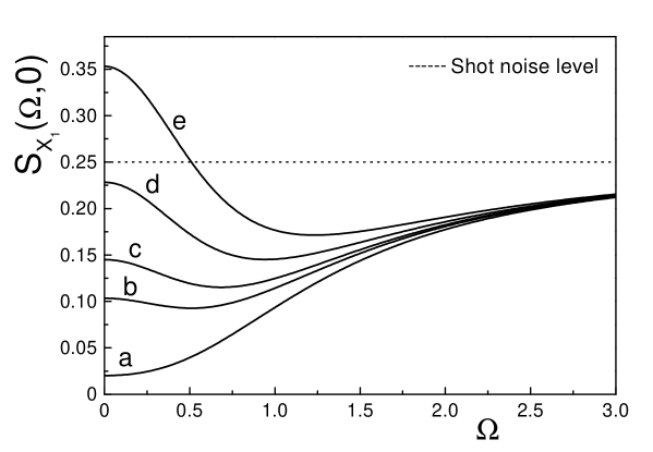
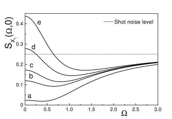
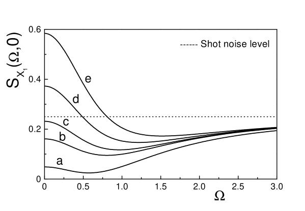
From Figs. 1-3 it follows that the change of the intensity of one light pulse gives a method for the control of squeezed spectra formation for another pulse and this control is effective if the intensity of the control pulse is much larger than that of the investigated pulse. While the intensity of the control pulse increases, the squeezing at the frequency for which the initial phase was chosen to be optimal, is destroyed. The suppression of the quadrature-component fluctuations for the investigated light pulse at higher intensities of the control pulse takes place in the frequency domain $\omega\approx 1/\tau_{r}$.

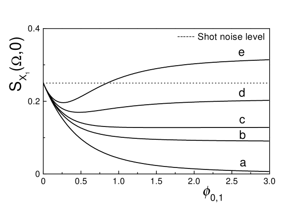
Squeezing spectra of the investigated pulse (85) for various frequencies $(\Omega=0$, $0.3$, $0.5)$ and different intensities of the control pulse as functions of the maximum nonlinear phase addition $\phi_{0,1}$ are shown in Figs. 4, 5, and 6, respectively. One can see from Figs. 4-6 that at higher intensities of the control pulse the spectral density under investigation reaches the minimum value in the domain $\phi_{0,1}\leq 1$ and then the spectral density does not practically change.

Figure 4: Fluctuation spectrum of the quadrature-squeezed component of the investigated pulse for the frequency $\Omega=0$ for the case of optimal initial phase $\varphi_{0,1}(t)$ chosen for $\Omega_{0}=0$ and for different intensities of the control pulse $\bar{n}_{0,2}/\bar{n}_{0,1}=0$ (a), $2$ (b), $3$ (c), $5$ (d), $8$ (e). Curves are calculated for the time moment $t=0$ and $\gamma_{1}=\gamma_{2}=2\tilde{\gamma}$.

Figure 5: The same as in Fig. 4 but for the frequency $\Omega=0.3$.

Figure 6: The same as in Fig. 4 but for the frequency $\Omega=0.5$.

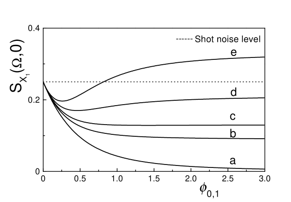
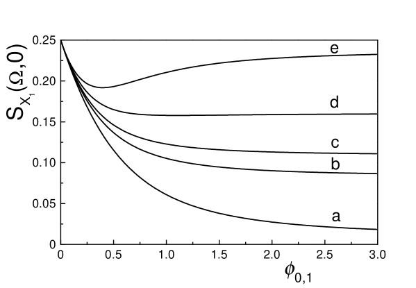
The appropriate for our purpose spectra can be also obtained by changing the intensity of control pulse and measuring the spectra for defined frequency $\Omega$ when the initial phase of the investigated pulse is chosen to be optimal for various $\Omega_{0}$. Such a dependence is displayed in Fig. 7. In some sense, the spectra shown in Figs. 4 and 7 are similar, and they demonstrate that the measurements carried out at frequencies, for which the initial phase was chosen optimal, give almost the same results. From Figs. 4-7 one can see that the XPM effect determines the domain of $\phi_{0,1}$ values where the spectral density of quadrature component fluctuations is independent on the intensity of the investigated pulse at the output of nonlinear medium.

Figure 7: Fluctuation spectrum of the quadrature-squeezed component of investigated pulse at the frequency $\Omega=0.5$ for the case of optimal initial phase $\varphi_{0,1}(t)$ chosen for $\Omega_{0}=0.5$ and for different intensities of the control pulse $\bar{n}_{0,2}/\bar{n}_{0,1}=0$ (a), $2$ (b), $3$ (c), $5$ (d), $8$ (e). Curves are calculated for the time moment $t=0$ and $\gamma_{1}=\gamma_{2}=2\tilde{\gamma}$.

6 Conclusion

We have developed the quantum theory of two USPs propagation in the nonlinear medium with inertial electronic Kerr nonlinearity. In the considered case, the propagating pulses are subject simultaneously to the SPM and XPM effects. The nonlinear medium is suggested to be lossless and dispersionless, that is, the pulse frequencies are off-resonances. Nevertheless, to develop in this case the consistent quantum theory of the SPM–XPM effect, it is necessary to take into account a finite time of nonlinear response. In the developed approach, we neglect thermal fluctuations of nonlinearity, and the causality principle is not violated for the observed values.

The nonlinear response time defines spectral width of quadrature-squeezed light [see Eqs. (80), (81)]. The level of suppression of quantum fluctuations depends on the nonlinear phase additions due to both the SPM and XPM phenomena.

It is shown that the frequency, at which the suppressions of fluctuations is maximum, can be controlled by adjusting the initial phase of the investigated light pulse and the intensity of another pulse.

The results of this paper can be used in the study of creation of the USPs in nonclassical states and in quantum non-demolition measurements using USPs.

The approach developed can be applied to generalize the theory of other quantum effects associated with the two-mode light propagation in the Kerr media (see references in [5]) to the case of pulse fields, for example, generation of polarization-squeezed light [15]. This study is in progress.

References

• [1] Tanas R 1984 in Coherence and Quantum Optics V Eds L Mandel and E Wolf (New York: Plenum Press) p. 645
• [2] Kitagawa M and Yamamoto Y 1986 Phys. Rev.A $\mathbf{34}$ 3974
• [3] Akhmanov S A, Belinsky A V, and Chirkin A S 1990 in New Physical Principles for Optical Information Processing (in Russian) Eds. S A Akhmanov and M A Vorontsov (Moscow: Nauka) p. 83
• [4] Volokhovsky V V and Chirkin A S 1997 Opt. Spektrosk. $\mathbf{82}$ 888
• [5] Tanas R 2001 SPIE Proc. of ICONO’2001 (in press)
• [6] Boivin L, Kärtner F X, and Haus H A 1994 Phys. Rev. Lett.$\mathbf{73}$ 240
• [7] Boivin L 1994 Phys. Rev.A $\mathbf{52}$ 754
• [8] Popescu F and Chirkin A S 1999 Pis’ma Zh. Éksp. Teor. Fiz. $\mathbf{69}$ 481; JETP Lett. $\mathbf{69}$ 516
• [9] Chirkin A S and Popescu F 2001 J. Russ. Laser Res. $\mathbf{22}$ 354
• [10] Chirkin A S and Popescu F 2001 in Quantum Communication, Computing, and Measurement 3  Eds P. Tombesi and O. Hiroto (New York: Kluwer Academic/ Plenum Publishers) p. 335 (Chirkin A S and Popescu F 2000 Preprint quant-ph/0010006)
• [11] Blow K J, Loudon R, and Phoenix S J D 1991 J. Opt. Soc. Am.B $\mathbf{8}$ 1750
• [12] Toren Mooki and Ben-Aryeh Y 1994  Quantum Opt. $\mathbf{9}$ 425
• [13] Akhmanov S A, Vysloukh V A, and Chirkin A S 1992 Optics of Femtosecound Laser Pulses, AIP, New York [1988 Supplemented translation of Russian original, Nauka, Moscow]
• [14] Joneckis L G and Shapiro J H 1993 J. Opt. Soc. Am.B $\mathbf{10}$ 1102
• [15] Chirkin A S, Orlov A A, and Paraschuk D Yu 1993 Kvant. Elektron. (Moscow) $\mathbf{20}$ 999 [1993 Sov. J. Quantum Electron. $\mathbf{23}$ 870]