Stability and instability in parametric resonance and quantum Zeno effect

Abstract

A quantum mechanical version of a classical inverted pendulum is analyzed. The stabilization of the classical motion is reflected in the bounded evolution of the quantum mechanical operators in the Heisenberg picture. Interesting links with the quantum Zeno effect are discussed.

An inverted pendulum is an ordinary classical pendulum initially prepared in the vertical upright position [1, 2, 3]. This is normally an unstable system, but can be made stable by imposing a vertical oscillatory motion to the pivot. In a few words, when the pivot is accelerated upwards the motion is unstable, while when it is accelerated downwards the motion can be stable: the periodic switch between these two situations can be globally stable or unstable depending on the values of some physical parameters. In particular, when the frequency of the oscillation is higher than a certain threshold, the system becomes stable. This result is a bit surprising at first sight, but can be given an interesting explanation in terms of the so-called parametric resonance [2].

In this Letter we shall study a system that can be viewed as a quantum version of the inverted pendulum. The system to be considered makes use of down-conversion processes interspersed with zones where a linear coupling takes place between the down-converted photon modes. It is similar to other examples previously analyzed [4, 5] in the context of the quantum Zeno effect [6], where the “measurement” is performed by a mode of the field on another mode. When the coupling between the two modes is large enough, the measurement becomes more effective and the dynamics gets stable: this is just a manifestation of the quantum Zeno effect, which consists in the hindrance of the quantum evolution caused by measurements. The very method of stabilization of the quantum system analyzed here is one of its most interesting features and the configuration we discuss is experimentally realizable in an optical laboratory. It is therefore of interest both for the investigation of the stable/unstable borderline for classical and quantum mechanical systems and their links with the quantum Zeno effect.

We consider a laser field (pump) of frequency $\omega_{p}$, propagating through a nonlinear coupler. The field is considered to be classical and the signal and idler modes are denoted by $a$ and $b$, respectively. We will assume that all modes are monochromatic and the amplitudes of the fields inside the coupler vary little during an optical period (SVEA approximation). The effective (time-dependent) Hamiltonian reads ($\hbar$=$1$)

$$H(t)=\omega_{a}a^{\dagger}a+\omega_{b}b^{\dagger}b+H_{\rm int}(t),$$ (1)

where the interaction Hamiltonian is given by

$$H_{\rm int}(t)=\left\{\begin{array}[]{ll}\Gamma(a^{\dagger}b^{\dagger}e^{-i\omega_{p}t}+abe^{i\omega_{p}t})&\mbox{if $0<t<\tau_{1}$},\\ \Omega(a^{\dagger}b+ab^{\dagger})&\mbox{if $\tau_{1}<t<\tau_{1}+\tau_{2}$}\end{array}\right.$$ (2)

and $H_{\rm int}(t+nT)=H_{\rm int}(t)$, with a period $T=\tau_{1}+\tau_{2}$. The nonlinear coupling constant $\Gamma$ is proportional to the second-order nonlinear susceptibility of the medium $\chi(2)$ [7], $\Omega$ to the overlap between the two modes [8] and $n=0,1,\cdots,N$ is an integer.

We require the matching conditions $\omega_{p}=\omega_{a}+\omega_{b}$ and $\omega_{a}=\omega_{b}$ [9]. The above Hamiltonian describes phase-matched down-conversion processes, for $nT<t<nT+\tau_{1}$, interspersed with linear interactions between signal and idler modes, for $nT+\tau_{1}<t<(n+1)T$. Since time is equivalent, within our approximations, to propagation length, our system can be thought of as a nonlinear crystal cut into $N$ pieces, in each of which $a,b$ photons are created in a down-conversion process. A similar configuration was considered in [4]. Between these pieces, no new photons are created by the laser beam, but the idler and signal modes (linearly) interact with each other, for instance via evanescent waves. See Fig. 1.

FIG. 1.: The system

By introducing the slowly varying operators $a^{\prime}=e^{i\omega_{a}t}a$, $b^{\prime}=e^{i\omega_{b}t}b$, the free part of the Hamiltonian (1) is transformed away and the Hamiltonian becomes (suppressing all primes for simplicity)

$$H(t)=\left\{\begin{array}[]{ll}H_{\rm u}\equiv\Gamma(a^{\dagger}b^{\dagger}+ab)&\mbox{if $0<t<\tau_{1}$},\\ H_{\rm s}\equiv\Omega(a^{\dagger}b+ab^{\dagger})&\mbox{if $\tau_{1}<t<\tau_{1}+\tau_{2}$},\end{array}\right.$$ (3)

with $H(t+nT)=H(t)$, yielding the equations of motion

$$\dot{a}=-i[a,H],\qquad\dot{b}=-i[b,H].$$ (4)

In terms of the variables

$$x_{\pm} = \frac{1}{2}[(a+a^{\dagger})\mp(b+b^{\dagger})],$$ (5)

$$p_{\pm} = -\frac{i}{2}[(a-a^{\dagger})\mp(b-b^{\dagger})],$$ (6)

which satisfy the equal-time commutation relations $[x_{+},p_{+}]=[x_{-},p_{-}]=i$, others${}=0$, the Hamiltonians become

$$H_{\rm u} = \frac{\Gamma}{2}[(p_{+}^{2}-x_{+}^{2})-(p_{-}^{2}-x_{-}^{2})],$$ (7)

$$H_{\rm s} = \frac{\Omega}{2}[(p_{+}^{2}+x_{+}^{2})-(p_{-}^{2}+x_{-}^{2})].$$ (8)

They describe two uncoupled oscillators, whose equations of motion are

$$\left\{\begin{array}[]{l}\dot{x}_{\pm}=-i[x_{\pm},H_{\rm u}]=\pm\Gamma p_{\pm}\\ \dot{p}_{\pm}=-i[p_{\pm},H_{\rm u}]=\pm\Gamma x_{\pm}\end{array}\right.\Longleftrightarrow\left\{\begin{array}[]{l}\ddot{x}_{\pm}-\Gamma^{2}x_{\pm}=0\\ \ddot{p}_{\pm}-\Gamma^{2}p_{\pm}=0\end{array}\right.,$$ (13)

(14)

$$\left\{\begin{array}[]{l}\dot{x}_{\pm}=-i[x_{\pm},H_{\rm s}]=\pm\Omega p_{\pm}\\ \dot{p}_{\pm}=-i[p_{\pm},H_{\rm s}]=\mp\Omega x_{\pm}\end{array}\right.\Longleftrightarrow\left\{\begin{array}[]{l}\ddot{x}_{\pm}+\Omega^{2}x_{\pm}=0\\ \ddot{p}_{\pm}+\Omega^{2}p_{\pm}=0\end{array}\right..$$ (19)

The first set of equations describes an unstable motion, the second set a stable one, around the equilibrium point $x=p=0$. Notice that the motion of $(x_{-},p_{-})$ is the time-reversed version of that of $(x_{+},p_{+})$. This is due to the fact that the two motions are governed by Hamiltonians with opposite sign in Eq. (8). Henceforth, we shall concentrate on the variables $(x_{+},p_{+})$ [the stability condition for $(x_{-},p_{-})$ is identical]. The solutions are

$$\pmatrix{x_{+}(\tau_{1})\cr p_{+}(\tau_{1})}=A_{\rm u}\pmatrix{x_{+}(0)\cr p_{+}(0)},$$ (20)

$$\qquad\qquad A_{\rm u}\equiv\pmatrix{\cosh(\Gamma\tau_{1})&\sinh(\Gamma\tau_{1})\cr\sinh(\Gamma\tau_{1})&\cosh(\Gamma\tau_{1})},$$ (21)

for the period governed by $H_{\rm u}$ and

$$\pmatrix{x_{+}(\tau_{2})\cr p_{+}(\tau_{2})}=A_{\rm s}\pmatrix{x_{+}(0)\cr p_{+}(0)},$$ (22)

$$\qquad\qquad A_{\rm s}\equiv\pmatrix{\cos(\Omega\tau_{2})&\sin(\Omega\tau_{2})\cr-\sin(\Omega\tau_{2})&\cos(\Omega\tau_{2})},$$ (23)

for that governed by $H_{\rm s}$. Remember that $T=\tau_{1}+\tau_{2}$ is the period of the Hamiltonian $H(t)$ in (3).

The dynamics engendered by (3) at time $t=NT$ (remember that $n=1,\ldots,N$) yields therefore

$$\pmatrix{x_{+}(NT)\cr p_{+}(NT)}=A^{N}\pmatrix{x_{+}(0)\cr p_{+}(0)},\qquad A\equiv A_{\rm s}A_{\rm u}.$$ (24)

These equations of motion have the same structure of a classical inverted pendulum with a vertically oscillating point of suspension [2], whose classical map is given by the product of two matrices $A_{\rm cl}\equiv A_{2}A_{1}$, with

$$A_{1} \equiv \pmatrix{\cosh(k_{1}\tau)&k_{1}^{-1}\sinh(k_{1}\tau)\cr k_{1}\sinh(k_{1}\tau)&\cosh(k_{1}\tau)},$$ (25)

$$A_{2} \equiv \pmatrix{\cos(k_{2}\tau)&k_{2}^{-1}\sin(k_{2}\tau)\cr-k_{2}\sin(k_{2}\tau)&\cos(k_{2}\tau)},$$ (26)

where the parameters $k_{1}$ and $k_{2}$ are subject to the physical condition $k_{1}>k_{2}>0$. Observe that our system has more freedoms: $\tau_{1}$ and $\tau_{2}$ are in general different and the parameters $\Omega$ and $\Gamma$ do not have to obey any additional constraint.

The global motion is stable or unstable, according to the value of $|\mbox{Tr}A|\lesseqgtr 2$ [2]. The stability condition $|\mbox{Tr}A|<2$ reads

$$|\mbox{Tr}A|/2=|\cos(\Omega\tau_{2})\cosh(\Gamma\tau_{1})|<1.$$ (27)

This relation is of general validity and holds for any value of the parameters $\Omega,\Gamma$ and $\tau_{i}$. The value of $|\mbox{Tr}A|/2$ is shown in Fig. 2a). A small-$\tau$ expansion (the physically relevant regime: see final discussion) yields

$$1-(\Omega^{2}\tau_{2}^{2}-\Gamma^{2}\tau_{1}^{2})/2+O(\tau^{4})<1,$$ (28)

so that the system is stable for $\Omega\tau_{2}>\Gamma\tau_{1}$ when $\tau_{2}\to 0$.

FIG. 2.: Stability condition (27) in parameter space. a) $|\mbox{Tr}A|/2$ vs $\Omega\tau_{2}$ and $\Gamma\tau_{1}$; b) Stability (Zeno) region.

It is interesting to discuss the stability condition just obtained for the $(x,p)$ variables in terms of the number of down-converted photons. To this end, let us look at some limiting cases. [Needless to say, the analysis could be done from the outset in terms of $n_{a}$ and $n_{b}$ and would yield an identical stability condition (27).] When $\Omega=0$ in (3) and following equations, only the down-conversion process takes place and both $n_{a}=a^{\dagger}a$ and $n_{b}=b^{\dagger}b$ grow exponentially with time. There is an exponential energy transfer from the pump to the $a,b$ modes. On the other hand, if $\Gamma=0$ and the system is prepared in any initial state (except vacuum, whose evolution is trivial), $n_{a}$ and $n_{b}$ oscillate in such a way that their sum is conserved (this is due to the property $[n_{a}+n_{b},H_{\rm s}]=0$). If both $\Omega$ and $\Gamma$ are nonvanishing, these two opposite tendencies (exponential photon production and bounded oscillations) compete in an interesting way. When $\Gamma\tau_{1}>\Omega\tau_{2}$, in the limit $\tau_{1}\to 0$, the exponential photon production dominates and there is no way of halting (or even hindering) this process: the (external) pump transmits energy to the $a,b$ modes. In terms of the $(x,p)$ variables, the stability condition (28) cannot be fulfilled and the oscillator variables move exponentially away from the origin. The opposite situation $\Omega\tau_{2}>\Gamma\tau_{1}$ is very interesting and displays some quite nontrivial aspects: The motion becomes stable and the pump does not transmit energy to the $a,b$ modes anymore (the two modes oscillate).

In general and for arbitrary values of all parameters, the action of $H_{\rm s}$ can be viewed as a sort of measurement [5, 10, 11], in the following sense: the $a$ mode performs an observation on the $b$ mode and vice versa, the photonic states get entangled and information on one mode is encoded in the state of the other one. For example, the condition $\Omega\tau_{2}=\pi/2$ yields an “ideal measurement” of one mode on the other one, for in such a case the states $|1_{a},0_{b}\rangle\leftrightarrow|0_{a},1_{b}\rangle$ evolve into each other. From this viewpoint, the stabilization regime just investigated can be considered as a quantum Zeno effect [6], in that the measurements essentially affect and change the original dynamics. In fact, if one considers $\Omega\tau_{2}$ as the “strength” of the measurement, by increasing (at fixed $\Omega\tau_{2}$) the frequency of measurements, i.e. by letting $\tau_{1}\to 0$, the system moves down along a vertical line in Fig. 2b) and enters a region of stability (Zeno region) from a region of instability. (Notice that it is not necessary to consider the $\tau_{1}=0$ limit (“continuous measurement”) in order to stabilize the dynamics; there is a threshold, given by the curve in Fig. 2 b), at which stability and instability interchange.) Analogously, at fixed $\Gamma\tau_{1}$, by moving along a horizontal line $\Omega\tau_{2}\to\pi/2$ the system enters a region of stability because the measurement becomes more “effective:” indeed, as emphasized before, $\Omega\tau_{2}=\pi/2$ is a $\pi$-pulse condition and leads to a very effective measurement of one mode on the other one. It is worth stressing that even an instantaneous measurement (projection) can be obtained by letting $\tau_{2}\to 0$, while keeping $\Omega\tau_{2}$ finite (the so-called impulse approximation in quantum mechanics), and in this case our system yields the standard formulation of the quantum Zeno effect.

It is interesting (and convenient from an experimental perspective) to consider a single-mode version of the Hamiltonian (3), in which the down-conversion process is replaced by a sub-harmonic generation process (degenerated parametric down conversion). The single-mode effective Hamiltonian reads

$$H(t)=\omega a^{{\dagger}}a+H_{\rm int}(t),$$ (29)

where the interaction Hamiltonians describing the unstable and stable part of the device are

$$H_{\rm int}=\left\{\begin{array}[]{ll}(\Gamma/2)(a^{{\dagger}2}e^{-2i\omega t}+a^{2}e^{2i\omega t})&\mbox{if $0<t<\tau_{1}$},\\ (\Omega/2)(a^{{\dagger}}a+aa^{\dagger})&\mbox{if $\tau_{1}<t<\tau_{1}+\tau_{2}$},\end{array}\right.$$ (30)

respectively and $H_{\rm int}(t+nT)=H_{\rm int}(t)$. By introducing the slowly varying operator $a^{\prime}=e^{i\omega_{a}t}a$, the free part of the Hamiltonian (29) is transformed away and the Hamiltonian becomes (suppressing again all primes)

$$H(t)=\left\{\begin{array}[]{ll}H_{\rm u}\equiv(\Gamma/2)(a^{\dagger 2}+a^{2})&\mbox{if $0<t<\tau_{1}$},\\ H_{\rm s}\equiv(\Omega/2)(a^{\dagger}a+aa^{\dagger})&\mbox{if $\tau_{1}<t<\tau_{1}+\tau_{2}$},\end{array}\right.$$ (31)

under which the equation of motion $\dot{a}=-i[a,H]$ follows.

In terms of the variables $x=(a+a^{{\dagger}})/\sqrt{2},p=-i(a-a^{{\dagger}})/\sqrt{2}$ the Hamiltonians read

$$H_{\rm u}=\frac{\Gamma}{2}(x^{2}-p^{2}),\quad H_{\rm s}=\frac{\Omega}{2}(x^{2}+p^{2}).$$ (32)

These Hamiltonians are identical to the two-mode versions (8) describing the decoupled mode $(x_{+},p_{+})$, apart from the substitution $\Gamma\to-\Gamma$. Hence, the stability condition is given again by Eq. (27), which is even in $\Gamma$. Also in this case one can talk of quantum Zeno, but the “measurement” is performed by the single mode on itself.

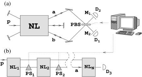
FIG. 3.: Experimental setup. (a) Possible experimental realization of the Hamiltonian (1)-(2). NL, nonlinear crystal; M${}_{i},(i=1,2)$, semitransparent mirrors; D_i, detectors; PBS, polarizing beamsplitter. (b) Possible experimental realization of the Hamiltonian (29)-(30). NL${}_{i}(i=1,\ldots,N)$, nonlinear crystals; PS_i, phase shifters; D₃, detector. The dotted lines indicate which elements are computer controllable.

It is interesting to discuss a possible experimental realization of the two situations considered in this Letter. The experimental arrangement sketched in Fig. 3(a) corresponds to the two-mode (nondegenerate) case, whereas that sketched in Fig. 3(b) to the single-mode (degenerate) case. In Fig. 3(a) a type II down-conversion process generates two orthogonally polarized beams of down-converted light of the same frequency. The two beams are mixed using a polarizing beamsplitter PBS. The stable part of the evolution of the system is realized by two successive passes of the beams through the beamsplitter. Its reflection coefficient, and hence $\Omega\tau_{2}$, is adjusted by rotating it. Mirrors and semitransparent mirrors keep sending the beams through the crystal many times. A successful stabilization of the unstable system is manifested in the decrease of the rate of photon registrations at detectors $D_{1}$, $D_{2}$ at a certain position of the beamsplitter PBS. A different setup is sketched in Fig. 3(b), where $N$ processes of subharmonic generation take place in $N$ nonlinear crystals with controlled phase shifters in between them. For appropriately chosen phase shifts $\theta_{i}=(\Omega\tau_{2}+C_{i})\bmod 2\pi$, where $C_{i}$ are $N-1$ phase shifts intrinsic to the actual experimental arrangement (given by distances between crystals, etc.), the generation of the subharmonic wave is suppressed.

In order to give a reasonable estimate of the value of the coupling constant $\Gamma$, consider that, due to the correspondence principle, the gain of classical and quantum parametric amplifiers must be the same; therefore one can use the well-known classical formula for the nonlinear coupling parameter $\Gamma_{c}$ governing the space evolution inside the nonlinear medium, which in MKS units reads

$$\Gamma_{c}^{2}=\frac{\eta^{3}}{2}\chi(2)^{2}\omega_{a}\omega_{b}I_{p}.$$ (33)

Here $\eta$ is the impedance of the medium, $\chi(2)$ is the second-order susceptibility, $\omega_{a}$ and $\omega_{b}$ are the frequencies of modes $a$ and $b$, respectively, and $I_{p}$ is the intensity of the pump beam. The following numerical values could be typical for a performed experiment: $\eta\approx 220\Omega$, $\chi(2)\approx 2\times 10^{-23}$ CV^-2, $\omega_{a}=\omega_{b}\approx 3\times 10^{15}$s^-1 and $I_{p}\approx 10^{5}$Wm^-2. Hence the nonlinear coupling parameter is of the order of $\Gamma_{c}\approx 0.1$m^-1. Reasonable lengths of nonlinear crystals are of the order of $l\approx 10^{-2}$m, so that the dimensionless product of interest can be estimated to be about

$$\Gamma\tau_{1}=\Gamma_{c}l\approx 0.001.$$ (34)

This means that the down-converted beam(s) ought to pass the nonlinear region many times in order to show an explosive increase of its (their) intensity(ies). This could be achieved by placing the nonlinear crystal in a resonator as shown in Fig. 3(a). However, in order to observe a significant change of the dynamics of the process in question due to the performed stabilization, a few passes might already turn out to be sufficient.

In conclusion, we have discussed a striking quantum-optical analogue of a well-known classical unstable system. By interspersing the nonlinear regions with regions of suitably chosen linear evolution, the global dynamics of our system can become stable and the generation of down-converted light can be strongly suppressed. This behavior has an interesting interpretation in terms of the quantum Zeno effect: by increasing the “strength” of the observation performed by the $a$ mode on the $b$ mode and vice versa, in the sense discussed before, the evolution is frozen and the system tends to remain in its initial state. This phenomenon is somewhat counterintuitive: in the setups in Fig. 3, even though the beams are forced to go through the crystal many times, no exponential photon production takes place. The experiment seems feasible and its realization would illustrate an interesting aspect related to the stabilization of a seemingly explosive behavior.

- [1] A. Stephenson, Philos. Mag. 15, 233 (1908); P.L. Kapitza, Collected papers, ed. by Ter Haar (Pergamon Press, London, 1965) Vol. 2, p. 714.
- [2] V.I. Arnold, Mathematical Methods of Classical Mechanics (Springer-Verlag, Berlin, 1989) p. 121; V.I. Arnold, Ordinary Differential equations (Springer-Verlag, Berlin, 1992) p. 263.
- [3] J.G. Fenn, D.A. Bayne and B.D. Sinclair, Am. J. Phys. 66, 981 (1998) and references therein.
- [4] A. Luis and J. Peřina, Phys. Rev. Lett. 76, 4340 (1996); A. Luis and L. L. Sánchez–Soto, Phys. Rev. A57, 781 (1998); K. Thun and J. Peřina, Phys. Lett. A249, 363 (1998).
- [5] J. Řeháček, J. Peřina, P. Facchi, S. Pascazio, and L. Mišta, Phys. Rev. A62, 13804 (2000).
- [6] A. Beskow and J. Nilsson, Arkiv für Fysik 34, 561 (1967); L.A. Khalfin, Zh. Eksp. Teor. Fiz. Pis. Red. 8, 106 (1968) [JETP Letters 8, 65 (1968)]; B. Misra and E. C. G. Sudarshan, J. Math. Phys. 18, 756 (1977).
- [7] C. K. Hong and L. Mandel, Phys. Rev. A31, 2409 (1985).
- [8] M. L. Stich and M. Bass, Laser Handbook (North–Holland, Amsterdam, 1985), Chapter 4; Yariv and Yeh, Optical Waves in Crystals (J. Wiley, New–York, 1984); B. E. A. Saleh and M. C. Teich, Fundamentals of Photonics (J. Wiley, New–York, 1991), Section 7.4.B.
- [9] The latter matching condition can be relaxed at the cost of introducing a second classical pump wave of frequency and the Hamiltonian , for , in (2). Physically, this corresponds to replacing the linear exchange between modes and with the nonlinear process of difference frequency generation.
- [10] E. Mihokova, S. Pascazio and L.S. Schulman, Phys. Rev. A56, 25 (1997); L.S. Schulman, Phys. Rev. A57, 1059 (1998); S. Pascazio and P. Facchi, Acta Phys. Slovaca 49, 557 (1999); P. Facchi and S. Pascazio, Phys. Rev. A62, 23804 (2000).
- [11] It is interesting to notice that for infinitesimal the effective Hamiltonian of the system becomes just the sum of the unstable and stable Hamiltonians (3). Such Hamiltonians are well known in the field of quantum nondemolition measurements: G. J. Milburn, A. S. Lane, and D. F. Walls, Phys. Rev. A27, 2804 (1983).