Abstract

The higher order supersymmetric partners of the Schrödinger’s Hamiltonians can be explicitly constructed by iterating a simple finite difference equation corresponding to the Bäcklund transformation. The method can completely replace the Crum determinants. Its limiting, differential case offers some new operational advantages.

PACS:

03.65.Ge, 03.65.Fd, 03.65.Ca

Key-Words:

Supersymmetry, factorization, difference equations

Accepted for publication in Phys. Lett. A (2000)

1 Introduction

It is notable that while the exact solutions in general relativity fill already ample handbooks, the exactly solvable problems of quantum theory form still an exceptional area. Yet, it seems that they are just the “top of an iceberg”, an opinion recently confirmed by advances in the exact methods [1]. One of the simplest ways of obtaining new exactly solvable spectral problems in Schrödinger’s quantum mechanics is to look for pairs of quantum Hamiltonians coupled “supersymmetrically” by an intertwining operator $A_{1}$

$$H_{1}A_{1}=A_{1}H_{0}.$$ (1)

This equation should hold on a certain dense domain of the Hilbert space of states $\cal H$, assuring that the spectrum of $H_{0}$ yields some information about the spectrum of $H_{1}$ and vice versa. The best known cases of (1) occur in ${\cal H}={L}^{2}({\hbox{{\extra R}}})$, where $H_{0}$ and $H_{1}$ are the Schrödinger Hamiltonians

$$H_{0}=-\frac{1}{2}\frac{d^{2}}{dx^{2}}+V_{0}(x),\qquad H_{1}=-\frac{1}{2}\frac{d^{2}}{dx^{2}}+V_{1}(x),$$ (2)

and $A_{1}$, $A_{1}^{\dagger}$ are the first order differential operators

$$A_{1}=\frac{d}{dx}+\beta_{1}(x),\qquad A_{1}^{{\dagger}}=-\frac{d}{dx}+\beta_{1}(x).$$ (3)

By introducing (2) and (3) into (1), and after an elementary integration, one gets the Riccati equation for $\beta_{1}(x)$

$$-\beta^{\prime}_{1}(x)+\beta_{1}^{2}(x)=2[V_{0}(x)-\epsilon],$$ (4)

where $\epsilon$ is an arbitrary integration constant called the factorization energy (a terminology which does not imply that $\epsilon$ must be a physical energy). Simultaneously,

$$V_{1}(x)=V_{0}(x)+\beta^{\prime}_{1}(x).$$ (5)

Equations (4) and (5) are necessary and sufficient conditions for the Hamiltonians to be factorized as

$$H_{0}-\epsilon=\frac{1}{2}\,A_{1}^{{\dagger}}A_{1},\qquad H_{1}-\epsilon=\frac{1}{2}\,A_{1}A_{1}^{{\dagger}}.$$ (6)

The susy partners (5)–(6) appear in all quantum problems solvable by factorization [2]. An element of arbitrariness in this construction was explored in 1984 [3]; its presence in Witten’s susy quantum mechanics was noticed by Nieto [4]; links with the historical Darboux theory [5] were established by Andrianov et al [6].

The higher order intertwining was considered by Crum [7] (see also Krein [8], Adler and Moser [9]). In physical applications though, for a long time, the attention was focused mostly on the first order intertwining operator $A_{1}$ (see [10] and references quoted therein). The idea of the higher order $A_{1}$ reemerged in 80’tieth [11, 12] and it was systematically pursued since 1993 (see the works of Veselov and Shabat [13], Andrianov et al [14], Eleonsky et al [15], Bagrov and Samsonov [16], Fernández et al [17, 18], and one of us [19]). As it turns out, the higher order susy partners of an arbitrary $H_{0}$ can be generated just by iterating the Darboux transformation with different factorization constants $\epsilon$ (see interesting theorems by Bagrov and Samsonov in [16]). Formally, this can be done by introducing a higher order intertwiner constructed by means of the determinant formula of Crum [7], a method fundamentally important, though not very easy to apply. The purpose of this note is to explore a faster method based on the Bäcklund transformation [20] which operates very simply at the level of the $\beta$-functions (superpotentials) in equations (3)–(5). It consist just in applying the finite difference calculus, without caring about wave functions, differential equations, etc. Moreover, if applied to a sufficiently rich initial family of solutions to (4), it permits to recover the complete parametric dependence in all subsequent susy steps without the need of integrating any differential equations [21, 22, 23]. We also show that the differential case of the algorithm gives an entire susy hierarchy for a fixed $\epsilon$ just in terms of quadratures and algebraic operations.

2 The finite difference algorithm

The solutions of the Riccati equation (4), and the potentials (5), depend implicitly on the factorization energy $\epsilon\in{\hbox{{\extra R}}}$. We shall make explicit this dependence by writing $\beta_{1}(x,\epsilon)$ for the solutions to (4), and $V_{1}(x,\epsilon)$ for the corresponding susy partners of $V_{0}(x)$. Hence, the intertwiner in (1) reads $A_{1}(\epsilon)=d/dx+\beta_{1}(x,\epsilon)$, while the corresponding Hamiltonians are $H_{0}=(1/2)A_{1}^{\dagger}(\epsilon)A_{1}(\epsilon)+\epsilon$, and $H_{1}(\epsilon)=(1/2)A_{1}(\epsilon)A_{1}^{\dagger}(\epsilon)+\epsilon$. Notice that $H_{0}$ does not depend on $\epsilon$, yet it admits many different factorizations for many factorization energies $\epsilon$, each one defining a different intertwined Hamiltonian $H_{1}(\epsilon)$, with a different potential $V_{1}(x,\epsilon)$.

Let us fix now $\epsilon=\epsilon_{1}$, and consider one of these potentials:

$$V_{1}(x,\epsilon_{1})=V_{0}(x)+\beta_{1}^{\prime}(x,\epsilon_{1}).$$

Since $V_{1}(x,\epsilon_{1})$ is a susy partner of $V_{0}(x)$, the eigenfunctions $\psi_{1}$ of the Hamiltonian $H_{1}(\epsilon_{1})$ can be generated from the eigenfunctions $\psi_{0}$ of $H_{0}$ by using the operator $A_{1}(\epsilon_{1})$. It means simply that if $\psi_{0}(x,\epsilon)$ is a sufficiently smooth function and if $\psi_{1}(x,\epsilon)\propto A_{1}(\epsilon_{1})\psi_{0}(x,\epsilon)$, then:

$$H_{0}\psi_{0}(x,\epsilon)=\epsilon\psi_{0}(x,\epsilon)\Longrightarrow H_{1}(\epsilon_{1})\psi_{1}(x,\epsilon)=\epsilon\psi_{1}(x,\epsilon).$$ (7)

Notice that (7) does not require the square integrability of either $\psi_{0}$ or $\psi_{1}$. Nevertheless, if $\epsilon$ corresponds to one of the discrete spectrum eigenvalues $E$ of $H_{0}$, then $\psi_{0}$ can be chosen square integrable.

A question arises now, can $V_{1}(x,\epsilon_{1})$ be a convenient point of departure for the next susy step? The answer is positive and admits an explicit construction. In geometric form it was described by Adler as a mapping of complex polygons corresponding to the Bäcklund transformations [24] (see also Veselov and Shabat [13]). Its presence in the supersymmetric algorithm can be shown directly, using only the Riccati equation (4). Indeed, if $\beta_{1}(x,\epsilon)$ is a solution of (4), the function

$$u_{1}(x,\epsilon)=\exp{\left[-\int\beta_{1}(x,\epsilon)dx\right]}$$

satisfies $H_{0}u_{1}(x,\epsilon)=\epsilon\,u_{1}(x,\epsilon)$. Therefore, the function defined as

$$u_{2}(x,\epsilon_{1},\epsilon)=A_{1}(\epsilon_{1})u_{1}(x,\epsilon)=[\beta_{1}(x,\epsilon_{1})-\beta_{1}(x,\epsilon)]\exp\left[-\int\beta_{1}(x,\epsilon)dx\right]$$ (8)

satisfies $H_{1}(\epsilon_{1})u_{2}(x,\epsilon_{1},\epsilon)=\epsilon\,u_{2}(x,\epsilon_{1},\epsilon)$, and the function $\beta_{2}(x,\epsilon_{1},\epsilon)$ defined by

$$u_{2}(x,\epsilon_{1},\epsilon)=\exp\left[-\int\beta_{2}(x,\epsilon_{1},\epsilon)dx\right]$$ (9)

must fulfill the new Riccati equation:

$$-\beta_{2}^{\prime}(x,\epsilon_{1},\epsilon)+\beta_{2}^{2}(x,\epsilon_{1},\epsilon)=2[V_{1}(x,\epsilon_{1})-\epsilon].$$ (10)

Reading back (9) and using (8) one has

$$\beta_{2}(x,\epsilon_{1},\epsilon)=-\frac{d}{dx}\ln{u_{2}(x,\epsilon_{1},\epsilon)}=\beta_{1}(x,\epsilon)-\frac{\beta_{1}^{\prime}(x,\epsilon_{1})-\beta_{1}^{\prime}(x,\epsilon)}{\beta_{1}(x,\epsilon_{1})-\beta_{1}(x,\epsilon)},$$

and using again (4) one ends up with an algebraic expression

$$\beta_{2}(x,\epsilon_{1},\epsilon)=-\beta_{1}(x,\epsilon_{1})-\frac{2(\epsilon_{1}-\epsilon)}{\beta_{1}(x,\epsilon_{1})-\beta_{1}(x,\epsilon)},$$ (11)

which is the basic element of the auto-Bäcklund transformation for the Korteweg-deVries (KdV) equation (as reported in [25], see also [20] and [26]). Thus, the $\beta$-functions of the second susy step are algebraically determined by a finite difference operation performed on the $\beta$-functions of the previous step. They give the next operator $A_{2}(\epsilon_{1},\epsilon)\equiv d/dx+\beta_{2}(x,\epsilon_{1},\epsilon)$ intertwining the Hamiltonian $H_{1}(\epsilon_{1})$ with a new one $H_{2}(\epsilon_{1},\epsilon)\equiv-(1/2)\,d^{2}/dx^{2}+V_{2}(x,\epsilon_{1},\epsilon)$,

$$H_{2}(\epsilon_{1},\epsilon)\,A_{2}(\epsilon_{1},\epsilon)=A_{2}(\epsilon_{1},\epsilon)\,H_{1}(\epsilon_{1}),$$ (12)

where

$$V_{2}(x,\epsilon_{1},\epsilon)=V_{1}(x,\epsilon_{1})+\beta_{2}^{\prime}(x,\epsilon_{1},\epsilon).$$ (13)

Quite obviously (1) and (12) imply

$$H_{2}(\epsilon_{1},\epsilon)\,{\cal A}_{2}={\cal A}_{2}\,H_{0},$$

where ${\cal A}_{2}=A_{2}(\epsilon_{1},\epsilon)\,A_{1}(\epsilon_{1})$. In [13, 24] the method has been applied to deform the cyclic supersymmetric chains, but we shall show that it can replace completely all other techniques in constructing quite arbitrary susy sequences.

Indeed, the method can be now repeated by induction, leading to the sequence of first order intertwining operators

$$A_{k}(\epsilon)\equiv\frac{d}{dx}+\beta_{k}(x,\epsilon),\qquad k=1,2,...,n,$$ (14)

where each $\beta_{k},\,k\geq 2,$ is simply the result of a finite difference operation performed on $\beta_{k-1}$:

$$\beta_{k}(x,\epsilon)=-\beta_{k-1}(x,\epsilon_{k-1})-\frac{2(\epsilon_{k-1}-\epsilon)}{\beta_{k-1}(x,\epsilon_{k-1})-\beta_{k-1}(x,\epsilon)}.$$ (15)

We have adopted here a shortcut notation making explicit only the dependence of $A_{k}$ and $\beta_{k}$ on the factorization constant introduced in the very last step, keeping implicit the dependence on the previous factorization constants (henceforth, the same criterion will be used for any other symbol depending on $k$ factorization energies):

$$A_{k}(\epsilon)\equiv A_{k}(\epsilon_{1},...,\epsilon_{k-1},\epsilon),\quad\beta_{k}(x,\epsilon)\equiv\beta_{k}(x,\epsilon_{1},...,\epsilon_{k-1},\epsilon).$$

The $\beta_{k}$ functions constructed at each next susy step automaticaly solve the Riccati equation with the potential $V_{k-1}$ of the previous step

$$-\beta_{k}^{\prime}(x,\epsilon)+\beta_{k}^{2}(x,\epsilon)=2[V_{k-1}(x,\epsilon_{k-1})-\epsilon],$$ (16)

or equivalently

$$-\beta_{k}^{\prime}(x,\epsilon)+\beta_{k}^{2}(x,\epsilon)=\beta_{k-1}^{\prime}(x,\epsilon_{k-1})+\beta_{k-1}^{2}(x,\epsilon_{k-1})+2(\epsilon_{k-1}-\epsilon)$$ (17)

permitting to define the new potential

$$V_{k}(x,\epsilon)=V_{k-1}(x,\epsilon_{k-1})+\beta_{k}^{\prime}(x,\epsilon).$$ (18)

In the resulting sequence of the new Hamiltonians

$$H_{k}(\epsilon)=-\frac{1}{2}\frac{d^{2}}{dx^{2}}+V_{k}(x,\epsilon)=\frac{1}{2}A_{k}(\epsilon)A^{\dagger}_{k}(\epsilon)+\epsilon,\qquad k=1,2,...,n$$ (19)

each next is intertwined with the previous one,

$$H_{k}(\epsilon)\,A_{k}(\epsilon)=A_{k}(\epsilon)\,H_{k-1}(\epsilon_{k-1}),\qquad H_{0}(\epsilon_{0})\equiv H_{0}.$$ (20)

All of them are the higher order susy partners of the initial $H_{0}$

$$H_{k}(\epsilon)\,{\cal A}_{k}={\cal A}_{k}\,H_{0},$$ (21)

(compare with [9]) where ${\cal A}_{k}$ is the higher order intertwining operator obtained in the factorized form:

$${\cal A}_{k}\equiv A_{k}(\epsilon)A_{k-1}(\epsilon_{k-1})\cdots A_{2}(\epsilon_{2})A_{1}(\epsilon_{1}).$$ (22)

(Here we follow our notation, making explicit the dependence of each $A_{k}$ on its last factorization energy.) Once having the sequence of superpotentials $\beta_{k}(x,\epsilon)$, constructed by the algorithm (15), it is easy to determine the new eigenfunctions $u_{k}(x,\epsilon)$ injected by the process into the Hamiltonians $H_{k-1}(\epsilon_{k-1})$. Indeed, the $u_{k}(x,\epsilon_{k})$ are defined by the first order differential equations

$$A_{k}(\epsilon)\,u_{k}(x,\epsilon)=\frac{d}{dx}u_{k}(x,\epsilon)+\beta_{k}(x,\epsilon)u_{k}(x,\epsilon)=0,\qquad k=1,2,...,n.$$ (23)

Up to now we have maintained implicit the element of arbitrariness in the $\beta$-functions at every recurrence step. However, the true advantages of the method can be seen if $\beta_{1}(x,\epsilon)$ is wider than just a particular solution of (4). Indeed, for each fixed $\epsilon$, we have to our disposal the general solution of the Riccati equation (16), i.e., an entire one-parametric family of functions. Thus, e.g., the general solution of (4), for a given $\epsilon_{1}$, depends on an additional integration parameter $\lambda_{1}$. Given any particular solution $\beta_{1p}(x,\epsilon_{1})$, the general one is obtained by an elementary transformation:

$$\beta_{1}(x,\epsilon_{1})=\beta_{1p}(x,\epsilon_{1})-\frac{d}{dx}\ln\left[\lambda_{1}-\int\exp\left\{2\int^{x}\beta_{1p}(y,\epsilon_{1})\,dy\right\}dx\right]\equiv\beta(x,\epsilon_{1},\lambda_{1}).$$ (24)

Now, the algorithm (11) can be interpreted as an operation on two classes of functions $\beta_{1}(x,\epsilon)$ and $\beta_{1}(x,\epsilon_{1})$: an arbitrary member of the class $\beta_{1}(x,\epsilon)$ subtracted from an arbitrary member of $\beta_{1}(x,\epsilon_{1})$ in the denominator of (11). Quite similarly, the general iteration step (15) can be applied for $\beta_{k-1}(\epsilon)$ and $\beta_{k-1}(\epsilon_{k-1})$ meaning any two superpotentials of the previous step, the only condition stating that they must solve the corresponding Riccati equation with the same potential $V_{k-2}$ (a fact which is automaticaly assured in the iterative process). If so, the method accumulates the integration constants, permitting to recover the full parametric dependence on the $n$-th susy potentials in a purely algebraic way. Thus, e.g., $\beta_{2}(x,\epsilon):=\beta(x;\epsilon_{1},\epsilon;\lambda_{1},\lambda)$ with the dependence on $\epsilon_{1},\lambda_{1},\epsilon,\lambda$ inherited from the previous step ($\lambda_{1}$ and $\lambda$ selecting two solutions among the elements of the families $\beta_{1}(x,\epsilon_{1})$ and $\beta_{1}(x,\epsilon)$ respectively). In general, our algorithm yields $\beta_{k}(x,\epsilon):=\beta(x;\epsilon_{1},...,\epsilon_{k-1},\epsilon;\lambda_{1},...,\lambda_{k-1},\lambda)$ where the parameters $\epsilon,\lambda$ will be varied to perform the next step, whereas $\epsilon_{1},...,\epsilon_{k-1},\lambda_{1},...,\lambda_{k-1}$ will stay fixed. In what follows, we shall employ the symbols $\beta_{k}(x,\epsilon)$ whenever wanting to abbreviate, but we shall hold the dependence on the accumulated integration constants $\epsilon_{1},...,\epsilon_{k-1},\lambda_{1},...,\lambda_{k-1}$ if necessary. Let us now introduce the functions:

$$\Omega_{k}(x,\epsilon)=\cases{\beta_{1}(x,\epsilon),\quad\mbox{\rm for $k=1$};\cr\cr\beta_{k}(x,\epsilon)+\beta_{k-1}(x,\epsilon_{k-1}),\quad\mbox{\rm for $k\geq 2$}.\cr}$$ (25)

Observe their fractal structure accumulating the finite difference derivatives (compare with [13])

$$\Omega_{k}(x,\epsilon_{k})=-\frac{2(\epsilon_{k-1}-\epsilon_{k})}{\Omega_{k-1}(x,\epsilon_{k-1})-\Omega_{k-1}(x,\epsilon_{k})},\quad\quad k\geq 2.$$ (26)

Now, (15) can be rewritten as $\beta_{k}(x,\epsilon)=\Omega_{k}(x,\epsilon)-\beta_{k-1}(x,\epsilon_{k-1})$. For example, for $k=2$ we get (11), while for $k=3$ we have

$$\hskip-25.6073pt\beta(x;\epsilon_{1},\epsilon_{2},\epsilon_{3};\lambda_{1},\lambda_{2},\lambda_{3})\!\! \!\!=\!\! \!\!\beta(x;\epsilon_{1};\lambda_{1})+\frac{2(\epsilon_{1}-\epsilon_{2})}{\beta(x;\epsilon_{1};\lambda_{1})-\beta(x;\epsilon_{2};\lambda_{2})}$$ (27)

$$\!\!\!+\frac{\epsilon_{2}-\epsilon_{3}}{\displaystyle\frac{\epsilon_{1}-\epsilon_{2}}{\beta(x;\epsilon_{1};\lambda_{1})-\beta(x;\epsilon_{2};\lambda_{2})}-\frac{\epsilon_{1}-\epsilon_{3}}{\displaystyle\beta(x;\epsilon_{1};\lambda_{1})-\beta(x;\epsilon_{3};\lambda_{3})}}.$$

As one can also notice, the “$n$-susy potentials” $V_{n}(x)$, present the different fractal structures for $n$ even and odd. Summarizing:

$$V_{n}(x,\epsilon_{n})=V_{0}(x)+\sum_{k=1}^{n}\beta_{k}^{\prime}(x,\epsilon_{k})=V_{0}(x)+\sum_{k=1}^{n}\left[\cos^{2}\left(\frac{(k+n)\pi}{2}\right)\right]\frac{d}{dx}\Omega_{k}(x,\epsilon_{k}).$$ (28)

This expression has been already applied to simplify the study of $n$-susy partners of the harmonic oscillator [17] and the Coulomb potential [19]. Notice now that when $\lambda_{k}=\lambda_{k-1}$, and taking the limit $\epsilon_{k-1}\to\epsilon$ in (15), the method produces a differential algorithm (a confluent susy operation)

$$\beta^{\rm conf}_{k}(x,\epsilon)=-\beta_{k-1}(x,\epsilon)-{2}\left(\frac{\partial\beta_{k-1}(x,\epsilon)}{\partial\epsilon}\right)^{-1},$$ (29)

which can be freely iterated. Likewise, the finite differences can be replaced by the $\epsilon$-derivatives in one or more places of the fractal formulae (27). The mechanism has been implicitly applied by Stalhoffen (see Section III of [23]), in the context of Crum’s determinant.

3 Simple and confluent operations

The difference-differential algorithms (15), (29) simplify remarkably the construction of transparent wells [1, 22, 23]. In fact, the Riccati equation (4) for $V_{0}(x)=0$ has the general solution

$$\beta_{1}(x;\epsilon;\alpha)=-\sqrt{2\epsilon}\,\cot[\sqrt{2\epsilon}\,(x-\alpha)],$$ (30)

with four different real 1-susy branches: S (singular), R (regular), P (periodic), and N (null), for different (real or complex) values of $\epsilon$ and $\alpha$ (see Table I). For example, the regular case (R) leads to the modified Pöschl-Teller potential $V_{1}^{R}(x,\epsilon,b)=-\kappa^{2}/\cosh^{2}[\kappa(x+b)]$, while the null case (N) corresponds to the potential barrier $V_{1}^{N}(x,\epsilon=0,a)=(x-a)^{-2}$. All of them are particular cases of the Weierstrass $\wp$-function:

$$V_{1}(x;\epsilon;\alpha)=\wp(x+\alpha,3(4\epsilon/3)^{2},(4\epsilon/3)^{3})+\frac{2\epsilon}{3}.$$ (31)

TABLE I. The four different real superpotentials $\beta_{1}$ coming out from (30), depending on the values of $\epsilon$ and the integration parameter $\alpha$. In each case S means singular, R regular, ${\rm P}$ periodic, and N null. The parameters $a$ and $b$ are arbitrary real numbers.

Case	$\epsilon$	$\sqrt{2\epsilon}$	$\alpha$	$\beta_{1}(x,\epsilon)$
S	$\epsilon<0$	$i\sqrt{2|\epsilon|}=i\kappa$	$a$	$-\kappa\,\coth[\kappa(x-a)]$
R	$\epsilon<0$	$i\sqrt{2|\epsilon|}=i\kappa$	$\displaystyle-b-\frac{i\pi}{2\kappa}$	$-\kappa\,\tanh[\kappa(x+b)]$
${\rm P}$	$\epsilon>0$	$\sqrt{2\epsilon}=k$	$a$	$-k\,\cot[k(x-a)]$
N	$0$	$0$	$a$	$\displaystyle-\frac{1}{x-a}$

By applying the algorithm (11) to the superpotentials R and S as given in Table I, one immediately gets the transparent double wells in form of the quadratic Bargmann potentials [26] (see Figure 1)

$$V_{2}(x,\epsilon_{2})=-(\kappa_{1}^{2}-\kappa_{2}^{2})\,\,\frac{\kappa_{1}^{2}\,\,{\rm csch}^{2}\,[\kappa_{1}(x+b)]+\kappa_{2}^{2}\,\,{\rm sech}^{2}\,[\kappa_{2}(x-a)]}{(\,-\kappa_{1}\coth\,[\kappa_{1}(x+b)]+\kappa_{2}\tanh\,[\kappa_{2}(x-a)]\,)^{2}}.$$ (32)

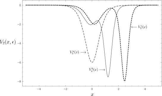
Figure 1: The double transparent wells (32) illustrate an application of the auto-Bäcklund transformation (11). The figure shows different members of the 2-susy family $V_{2}(x,\epsilon_{2},\epsilon_{1})$ for $\epsilon_{1}=-4$, $\epsilon_{2}=-1$, with integration parameters (a) $a=b=0$, (b) $a=0.254$, $b=-1.018$, and (c) $a=0.565$, $b=-2.262$.

The double wells (32) are well known in supersymmetry, but the use of the Bäcklund transformation makes the derivation considerably simpler, explaining also their place in the theory of the KdV equation, $v_{t}-6vv_{x}+v_{xxx}=0$. As a matter of fact, all the transparent $n$-susy wells can be now reinterpreted as the instantaneous forms of the multisoliton solutions propagating according to KdV (thus, e.g., the 2-susy potentials (32) originate the propagating soliton pairs [27]). Presumably, the susy partners of an arbitrary $V_{0}(x)$ generate as well the traveling “solitonic deformations” on a more general, non-null background.

The operational advantages of the differential algorithm (29) deserve as much attention. The application of the finite difference algorithm to the null wells is so easy, because for $V_{0}=0$ one knows the solutions of the Riccati eq. (4) for any $\epsilon$. For non-null $V_{0}$, (11) can be applied efficiently only if one knows at least two solutions of (4) for two different “factorization energies” $\epsilon$ (compare [17], [19]). For a general $V_{0}$, however, this is not granted. It is therefore interesting, that the difficulty is circumvented by the differential algorithm (29) which gives an easy access to higher order susy steps even if one starts from just one superpotential $\beta_{k}(x,\epsilon)$ for a fixed $\epsilon$. Indeed, by taking the limit $\epsilon\rightarrow\epsilon_{k-1}$, one reduces (17) to the following equation for $\beta_{k}=\beta_{k}(x,\epsilon=\epsilon_{k-1})$:

$$-\beta_{k}^{\prime}+\beta_{k}^{2}=\beta_{k-1}^{\prime}+\beta_{k-1}^{2},\quad k=2,3,...,$$ (33)

which has the particular solution $\beta_{k}=-\beta_{k-1}$ and integrates easily yielding:

$$\beta_{k}\! \!=\! \!-\beta_{k-1}+\frac{{e}^{-2\int\beta_{k-1}dx}}{\Gamma_{k}-\int{e}^{-2\int\beta_{k-1}dx}dx}$$ (34)

$$\!=\! \!-\beta_{k-1}-\frac{d}{dx}\ln\left[\Gamma_{k}-\int{{e}^{-2\int\beta_{k-1}dx}dx}\right].$$

Note that the right hand side of (34) depends essentially just on one integration constant. The recurrence (33) acquires even simpler form in terms of the new ‘key functions’ $B_{n}=\exp(-\int\beta_{n}dx+c_{n})$ (the integration constants $K_{n}=\exp c_{n}$ are superfluous to determine $\beta_{n}$). In fact, integrating both sides of (34), taking to the exponent, differentiating again, and choosing properly the (inessential) constants $K_{n}$, one has:

$$\frac{d}{dx}(B_{n}B_{n-1})=-B_{n-1}^{2}.$$ (35)

When this method is applied to $V_{0}(x)=x^{2}/2$ with $\epsilon=-1/2$, the first step recovers the Abraham-Moses oscillator [3], while the second step leads to the new 2-parametric family

$$V_{2}(x)=\frac{x^{2}}{2}-\frac{d^{2}}{dx^{2}}\ln\left[\Gamma_{2}-\int_{0}^{x}dy\ e^{y^{2}}\left(\Gamma_{1}-\frac{\sqrt{\pi}}{2}\ {\rm erf\,}x\right)^{2}\right],$$ (36)

which are different from the potentials discussed in [18], because they appear for a fixed $\epsilon$ and do not add 2 new spectral levels to $V_{0}$; we therefore propose to call them the 2-nd order Abraham-Moses potentials. The detailed analysis shows that (36) are singular unless $\Gamma_{1}=\frac{1}{2}\,\sqrt{\pi}$ and $\Gamma_{2}\geq\frac{1}{4}\,\sqrt{\pi}\,\ln 2$, or $\Gamma_{1}=-\frac{1}{2}\,\sqrt{\pi}$ and $\Gamma_{2}\leq-\frac{1}{4}\,\sqrt{\pi}\,\ln 2$. A nonsingular case with $\Gamma_{1}=\frac{1}{2}\,\sqrt{\pi}$ and $\Gamma_{2}=0.308$ is shown in Figure 2. The higher order Abraham-Moses functions can be as easily obtained in terms of (34). Generically, our algorithm is close to the nice idea of Leble [28] (though Leble did not construct the non-trivial contributions for $\delta=\epsilon-\epsilon_{k-1}=0$).

Figure 2: The solid line is a nonsingular 2-susy confluent partner for the harmonic oscillator with factorization energy $\epsilon=-1/2$ (equation (36)), for $\Gamma_{1}=\sqrt{\pi}/2$ and $\Gamma_{2}=0.308$. The dashed line represents the harmonic oscillator potential $x^{2}/2$.

An equally interesting application of the confluent formula (29) arises for the periodic superpotential ${\rm P}$ in Table I. In this case, the first order susy partner is given by

$$V_{1}^{\rm conf}(x,\epsilon)=V_{1}(x,\epsilon)=\frac{k^{2}}{\sin^{2}[k(x-a)]},$$ (37)

while the corresponding second order susy step leads to

$$V_{2}^{\rm conf}(x,\epsilon)=8k^{2}\,\,\frac{1-\cos\,[2k(x-a)]-k(x-a)\,\sin\,[2k(x-a)]}{(\,\sin\,[2k(x-a)]-2k(x-a)\,)^{2}}.$$ (38)

Notice that (37) is a periodic potential with singularities at the points $x_{n}=a+2n/k$, $n\in\hbox{{\extra Z}}$, while $V_{2}^{\rm conf}(x,\epsilon)$ has only one singularity. The confluent susy step (29) has removed all the singularities from $V_{1}^{\rm conf}(x,\epsilon)$ except that placed on $x=a$. The potential (38) has been plotted on Figure 3 (dashed curve) for $a=7,k=1/\sqrt{2}$. Observe that we have rederived the Stahlhofen function, but the method is simpler (see equations (50) and (40) of [23]). Moreover, some other potentials with analogous properties can be immediately obtained. Our Figure 3 reports the fourth order confluent potential $V_{4}^{\rm conf}(x,\epsilon)$, with $a=-7,k=1/\sqrt{2}$. Notice the appearance of two new symmetric singularities.

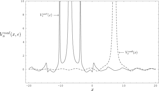
Figure 3: Examples of null, confluent $n$-susy potentials descending from the (P)-branch: $V_{2}^{\rm conf}(x)\equiv V_{2}^{\rm conf}(x;0.25;7)$, and $V_{4}^{\rm conf}(x)\equiv V_{4}^{\rm conf}(x;0.25;-7)$. For $n$ even in (28), the number of singularities grows with $n$ producing potentials of Stalhoffen type. The odd cases have always an infinite number of singularities.

As becomes obvious, for the periodic superpotentials $\beta_{1}$ in Table I, the method leads to two distinct classes of $n$-th order confluent potentials. For $n$ even, the periodic superpotential $\beta_{1}$ does not contribute directly to the sum (28) (the term with $k=1$ vanishes). The resulting susy partners have only a finite number of singularities. On the other hand, for $n$ odd, the function $\beta_{1}$ contributes to the first term in the sum (28) and its global effect is never canceled. The corresponding susy partners $V_{1}^{\rm conf}(x,\epsilon)$ therefore have infinite sequences of singularities. This difference reflects the distinct fractal structure of (28) for $n$ even and odd. The possibility of mixed applications of (15) and (29) is open.

References

- [1] B.N. Zakhariev and V. M. Chabanov, Inverse Problems 13, R47 (1997)
- [2] E. Schrödinger, Proc. R. Irish Acad. A 46, 183 (1940); P.A.M. Dirac, The Principles of Quantum Mechanics, Oxford University Press (1947); L. Infeld and T.E. Hull, Rev. Mod. Phys. 23, 21 (1951)
- [3] B. Mielnik, J. Math. Phys. 25, 3387 (1984); D.J. Fernández C., Lett. Math. Phys. 8, 337 (1984)
- [4] M.M. Nieto, Phys. Lett. B 145, 208 (1984)
- [5] G. Darboux, C. R. Acad. Sci. Paris 94, 1456 (1882)
- [6] A.A. Andrianov, N.V. Borisov and M.V. Ioffe, Theor. Math. Phys. 61, 1078 (1985)
- [7] M.M. Crum, Quart. J. Math. 6, 121 (1955)
- [8] M.G. Krein, Dokl. Acad. Nauk. SSSR 113, 970 (1957)
- [9] M. Adler and J. Moser, Commun. Math. Phys. 61, 1 (1978)
- [10] L.J. Boya, Eur. J. Phys. 9, 139 (1988); N.A. Alves and E. Drigo Filho, J. Phys. A 21, 3215 (1988); D.J. Fernández C., J. Negro and M. A. del Olmo, Ann. Phys. 252, 386 (1996);
- [11] D.J. Fernández C., Master Thesis, Phys. Department, CINVESTAV-IPN (1984)
- [12] C.V. Sukumar, J. Phys. A 19, 2297 (1986)
- [13] A.P. Veselov and A.B. Shabat, Funct. Anal. Appl. 27, No. 2, 1 (1993)
- [14] A.A. Andrianov, M.V. Ioffe, F. Cannata and J-P. Dedonder, Int. J. Mod. Phys. A 10, 2683 (1995)
- [15] V.M. Eleonsky and V.G. Korolev, J. Phys. A 28, 4973 (1995); J. Phys. A 29, L241 (1996); Phys. Rev. A 55, 2580 (1997)
- [16] B.F. Samsonov, J. Phys. A 28, 6989 (1995); Mod. Phys. Lett. A 11, 1563 (1996); V.G. Bagrov and B.F. Samsonov, Theor. Math. Phys. 104, 356 (1995); J. Phys. A 29, 1011 (1996); Phys. Part. Nucl. 28, 374 (1997)
- [17] D.J. Fernández C, Int. J. Mod. Phys. A 12, 171 (1997); D.J. Fernández C., V. Hussin and B. Mielnik, Phys. Lett. A 244, 1 (1998); D.J. Fernández C. and V. Hussin, J. Phys. A: Math. Gen. 32, 3603-3619 (1999)
- [18] D.J. Fernández C., M.L. Glasser and L.M. Nieto, Phys. Lett. A 240, 15 (1998)
- [19] J.O. Rosas-Ortiz, J. Phys. A 31, L507 (1998); J. Phys. A 31, 10163 (1998)
- [20] C. Rogers and W.F. Shadwick, Bäcklund Transformations and Their Applicatios, Academic Press, N.Y. (1984)
- [21] B.N. Zakhariev and A.A Suzko, Direct and Inverse Problems, Springer-Verlag, Berlin (1990)
- [22] V.B. Matveev and M.A. Salle, Darboux Transformations and Solitons, Springer-Verlag, Berlin (1991)
- [23] A. Stahlhofen, Phys. Rev. A 51, 934 (1995)
- [24] V.E. Adler, Funct. Anal. Appl. 27, No. 2, 79 (1993); Physica D 73, 335 (1994)
- [25] H.D. Wahlquist and F. B. Estabrook, Phys. Rev. Lett. 31, 1386 (1973)
- [26] G.L. Lamb, Elements of Soliton Theory, John Wiley & Sons, N.Y. (1984)
- [27] F. Cooper, A. Khare and U. Sukhatme, Phys. Rep. 251, 267 (1995).
- [28] S.B. Leble, Computers Math. Appl. 35, 73 (1998).