Discrete Moyal-type Representations for a Spin

Abstract

In Moyal’s formulation of quantum mechanics, a quantum spin $s$ is described in terms of continuous symbols, i.e. by smooth functions on a two-dimensional sphere. Such prescriptions to associate operators with Wigner functions, $P$- or $Q$-symbols, are conveniently expressed in terms of operator kernels satisfying the Stratonovich-Weyl postulates. In analogy to this approach, a discrete Moyal formalism is defined on the basis of a modified set of postulates. It is shown that appropriately modified postulates single out a well-defined set of kernels which give rise to discrete symbols. Now operators are represented by functions taking values on $(2s+1)^{2}$ points of the sphere. The discrete symbols contain no redundant information, contrary to the continuous ones. The properties of the resulting discrete Moyal formalism for a quantum spin are worked out in detail and compared to the continuous formalism, and it is illustrated by the example of a spin $1/2$.

1 Introduction

The idea to represent quantum mechanics of a particle in phase space $\Gamma$ goes back to Wigner [1]. He established a one-to-one correspondence between a quantum state $|\psi\rangle$ in the particle Hilbert-space ${\cal H}$ and a real function

$$W_{\psi}(p,q)=\frac{2}{h}\int_{\Gamma}\,dx\,\psi^{*}(q+x)\psi(q-x)\exp[2ipx/\hbar]\,.$$ (1)

Its properties suggest an interpretation as a quasi-probability in phase space, the only ‘drawback’ being due to the negative values it may take. A more general framework for phase-space representations [2] of quantum states as well as operators ${\widehat{A}}$ is given by the relation

$$W_{\widehat{A}}(q,p)=\mbox{ Tr }\left[\widehat{\Delta}(q,p)\widehat{A}\right]\,,$$ (2)

with an operator kernel [3, 4]

$$\widehat{\Delta}(q,p)=2\widehat{D}(q,p)\,{\widehat{\Pi}}\,\widehat{D}^{\dagger}(q,p)\,,\qquad(q,p)\in\Gamma\,.$$ (3)

Here ${\widehat{\Pi}}:(\hat{q},\hat{p})\to(-\hat{q},-\hat{p})$ is the unitary, involutive parity operator while $\widehat{D}(q,p)$ describes translations in phase space [5]. If the operator $\widehat{A}$ is chosen as the density matrix of a pure state, $\widehat{A}={\hat{\rho}}_{\psi}=|\psi\rangle\langle\psi|$, Eq. (2) reduces to (1). The kernel $\widehat{\Delta}(q,p)$ can be derived from a set of conditions which a phase-space representation is required to satisfy (cf. below). It is intimately related to the behaviour of a function $W_{A}(q,p)$ under translations mapping the phase space $\Gamma$ onto itself. The map (2) from operators to functions ($\widehat{A}\to W_{A}$) has an important feature: its inverse, mapping functions to operators ($W_{A}\to\widehat{A}$), is mediated by the same kernel —in other words, the kernel $\widehat{\Delta}(q,p)$ is self-dual.

For a quantum spin, the symbol associated with an operator is a continuous function defined on a sphere ${\cal S}^{2}$, which is the phase space of classical spin. Now, instead of translations in planar phase space, it is the group $SU(2)$ of rotations which plays a dominant role when the Moyal formalism is set up. As for a particle, the set of Stratonovich-Weyl postulates [6] characterizes the symbols in an elegant way. For clarity, the postulates are now displayed in their familiar form for the continuous symbols:

$$\begin{array}[]{lll}{(S0)}&{\sf linearity}:&\widehat{A}\mapsto W_{A}~{}~{}~{}{\rm is~{}a~{}linear~{}one~{}to~{}one~{}map},\\ {(S1)}&{\sf reality}:&\begin{minipage}{199.16928pt} $W_{A^{\dagger}}({\bf n})=W_{A}^{*}({\bf n})\,,$ \end{minipage}\\ {(S2)}&{\sf standardisation}:&\begin{minipage}{28.45274pt} \vspace{0mm} $${\frac{2s+1}{4\pi}\int_{{\cal S}^{2}}W_{A}({\bf n})d{\bf n}=\mbox{ Tr }[\widehat{A}]\hfill}\,,$$ \end{minipage}\\ {(S3)}&{\sf traciality}:&\begin{minipage}{28.45274pt} $$\frac{2s+1}{4\pi}\int_{{\cal S}^{2}}W_{A}({\bf n})W_{B}({\bf n})d{\bf n}=\mbox{ Tr }[\widehat{A}\widehat{B}]\,,\hfill$$ \vspace{0mm} \end{minipage}\\ {(S4)}&{\sf covariance}:&\begin{minipage}{199.16928pt} $W_{g\cdot A}=W_{A}^{g}\,,\quad g\in SU(2)\,.$ \end{minipage}\end{array}$$

It is natural to have a linear relation between operators and symbols (S0), while (S1) implies that hermitean operators are represented by real functions. The third condition (S2) maps the identity operator to the constant function on phase space, and traciality (S3) ensures that the correspondence between operators and symbols is invertible. The covariant transformation of the symbols with respect to rotations $g\in SU(2)$ effectively introduces phase-space points as arguments of the symbols. The continuous Moyal representation for a spin [7, 8] compatible with these conditions can be based on a self-dual kernel $\widehat{\Delta}({\bf n})$ (cf. Sect.  2) in analogy to (2).

In order to have a consistent and full-fledged classical formalism it is necessary to introduce a product between symbols which keeps track of the non-commutativity of the underlying operators. This Moyal product [2], or twisted product, for two operators $\widehat{A}$ and $\widehat{B}$ expresses the $W_{AB}$ of the operator product $\widehat{A}\widehat{B}$ in terms the symbols $W_{A}$ and $W_{B}$,

$$W_{AB}({\bf n})=W_{A}({\bf n})\ast W_{B}({\bf n})=\int_{{\cal S}^{2}}\int_{{\cal S}^{2}}L({\bf n},{\bf m},{\bf k})W_{A}({\bf m})W_{B}({\bf k})d{\bf m}d{\bf k}\,,$$ (4)

with a function $L({\bf n},{\bf m},{\bf k})$ of three arguments given explicitly in [7], for example. The $\ast$ product is known to be associative.

Other continuous representations for a spin do exist, such as the Berezin symbols of spin operators [9] which are the analog of the $P$- and $Q$-symbols [5] for a particle. Instead of a single self-dual kernel, the Berezin symbols require however, a pair of two different kernels, dual to each other: one of the kernels maps operators to functions while its dual is needed for the inverse procedure. It will become clear later on that the self-dual and the dual approach correspond to defining orthogonal and non-orthogonal bases, respectively, in the vector space ${\cal A}_{s}$ of operators acting on the Hilbert space of a spin $s$. When slightly modifying the postulates of Stratonovich, they are also compatible with kernels which are not self-dual.

A common feature of these representations is the redundancy of the continuous symbols. When represented by a $(2s+1)\times(2s+1)$ matrix, a hermitean operator is fixed by the values of $(2s+1)^{2}$ real parameters. Consequently, the values of the symbols, continuous functions on the sphere, cannot all be independent—in other words, the information contained in a symbol is redundant. The discrete version of $P$- and $Q$-symbols for a spin $s$, introduced in [10, 11] as a means to reconstruct the quantum state of a spin, allows one to characterize a spin operator $\widehat{A}$ by using only the minimal number of parameters. In fact, a discrete symbol can be considered as living on a ‘discretized sphere,’ that is, as a function taking (real) values on a finite set of points on the sphere only. Such a formalism will be called a discrete Moyal-type formalism.

The purpose of the present paper is to develop the discrete Moyal formalism in analogy to the continuous one. In particular, the kernel and its dual defining the discrete symbols will be derived from a set of appropriate Stratonovich-type postulates. Subsequently, the properties of these symbols are studied in detail.

2 Continuous representations

Continuous self-dual kernel: Wigner symbols

The Stratonovich-Weyl correspondence for a spin $s$ is a rule associating with each operator $\widehat{A}\in{\cal A}_{s}$ on a Hilbert space ${\cal H}_{s}$ a function $W_{A}$ on the sphere ${\cal S}^{2}$, called its (Wigner-) symbol. Let us define it in analogy to Eq. (2), by means of a universal operator kernel $\widehat{\Delta}({\bf n})$, which can also be thought of as a field of operators on the sphere. Then, the first requirement (S0) is already satisfied, and the postulates (S1) to (S4) turn into conditions on the kernel:

$$\begin{array}[]{lll}{(C1)}&{\sf reality}:&\begin{minipage}{199.16928pt} ${\widehat{\Delta}}^{\dagger}({\bf n})={\widehat{\Delta}}({\bf n})\,,$ \end{minipage}\\ {(C2)}&{\sf standardisation}:&\begin{minipage}{28.45274pt} \vspace{0mm} $${\frac{2s+1}{4\pi}\int_{{\cal S}^{2}}d{\bf n}\,{\widehat{\Delta}}({\bf n})=\hat{I}\hfill}\,,$$ \end{minipage}\\ {(C3)}&{\sf traciality}:&\begin{minipage}{28.45274pt} $$\frac{2s+1}{4\pi}\int_{{\cal S}^{2}}d{\bf n}\mbox{ Tr }\left[{\widehat{\Delta}}({\bf n}){\widehat{\Delta}}({\bf m})\right]{\widehat{\Delta}}({\bf n})={\widehat{\Delta}}({\bf m})\,,\hfill$$ \vspace{0mm} \end{minipage}\\ {(C4)}&{\sf covariance}:&\begin{minipage}{199.16928pt} ${\widehat{\Delta}}(g\cdot{\bf n})={\widehat{U}}_{g}\,{\widehat{\Delta}}({\bf n})\,{\widehat{U}}_{g}^{\dagger}\,,\quad g\in SU(2)\,.$ \end{minipage}\end{array}$$

where the matrices ${\widehat{U}}_{g}$ are a unitary $(2s+1)$-dimensional irreducible representations of the group $SU(2)$.

The existence of a kernel ${\widehat{\Delta}({\bf n})}$ satisfying (C1-4) has been proven in [6] by explicit construction. The derivation in [7] starts by expanding the kernel in a basis associated with the eigenstates of the operator ${\bf\hat{s}}\cdot{\bf n}_{z}$,

$${\widehat{\Delta}({\bf n})}=\sum_{m,m^{\prime}=-s}^{s}Z_{mm^{\prime}}({\bf n})|m,{\bf n}_{z}\rangle\langle m^{\prime},{\bf n}_{z}|\,,$$ (5)

with unknown coefficients $Z_{mm^{\prime}}({\bf n})$. It follows from (C1-4) that one must have

$$Z_{mm^{\prime}}^{s}({\bf n})=\frac{\sqrt{4\pi}}{2s+1}\sum_{l=0}^{2s}\varepsilon_{l}\sqrt{2l+1}\left<\begin{array}[]{cc|c}s&l&s\\ m&m^{\prime}-m&m^{\prime}\end{array}\right>Y_{l,m^{\prime}-m}({\bf n})\,,$$ (6)

where $\varepsilon_{0}=1$ and $\varepsilon_{l}=\pm 1\,,l=1,\ldots,2s$, and the definition of Clebsch-Gordan coefficient given in [7] is used. Consequently, there are $2^{2s}$ different kernels which define a Stratonovich-Weyl correspondence rule.

A new and simple derivation of the kernel ${\widehat{\Delta}({\bf n})}$, independent of the argument given in [7], is presented now which has two important advantages. On the one hand, it will provide a form of the kernel similar to that one of a particle (3), which is interesting from a conceptual point of view. On the other hand, it will be possible to transfer this approach to a large extent to the case of the discrete Moyal formalism.

Expand the kernel in the eigenbasis of the operator $\hat{\bf s}\cdot{\bf n}$,

$$\widehat{\Delta}({\bf n})=\sum_{m,m^{\prime}=-s}^{s}\Delta_{mm^{\prime}}({\bf n})|m,{\bf n}\rangle\langle m^{\prime},{\bf n}|\,,$$ (7)

where the expansion coefficients $\Delta_{mm^{\prime}}$ are unknown so far. According to the reality condition (C1) they must satisfy $\Delta_{mm^{\prime}}({\bf n})=\Delta_{m^{\prime}m}^{*}({\bf n})$. In a first step, the numbers $\Delta_{mm^{\prime}}({\bf n})$ are shown not to depend on the label ${\bf n}$. Consider the transformation of $\widehat{\Delta}({\bf n})$ under a rotation $g$. According to (C4) one must have

$$\sum_{m,m^{\prime}=-s}^{s} \Delta_{mm^{\prime}}(g\cdot{\bf n})|m,g\cdot{\bf n}\rangle\langle m^{\prime},g\cdot{\bf n}|=$$ (8)

$$= {\widehat{U}}_{g}\,\widehat{\Delta}({\bf n})\,{\widehat{U}}_{g}^{\dagger}=\sum_{m,m^{\prime}=-s}^{s}\Delta_{mm^{\prime}}({\bf n})|m,R_{g}{\bf n}\rangle\langle m^{\prime},R_{g}{\bf n}|\,,$$

where ${\widehat{U}}_{g}|m,{\bf n}\rangle=|m,R_{g}{\bf n}\rangle=|m,g\cdot{\bf n}\rangle$ with a rotation matrix $R_{g}\in SO(3)$ representing $g\in SU(2)$ in $I\!\!R^{3}$. Consequently, one must have

$$\Delta_{mm^{\prime}}(g\cdot{\bf n})=\Delta_{mm^{\prime}}({\bf n})\,,$$ (9)

which is only possible if $\Delta_{mm^{\prime}}$ does not depend on ${\bf n}$. Consider next a rotation $g({\bf n})$ about the axis ${\bf n}$ by an angle $\varphi\in[0,2\pi)$, represented by the unitary ${\widehat{U}}_{g({\bf n})}=\exp(i{\bf n}\cdot\hat{\bf s}\varphi)$. The left-hand-side of (C4) is invariant under this transformation while the right-hand-side transforms:

$$\widehat{\Delta}(R_{g({\bf n})}{\bf n})=\widehat{\Delta}({\bf n})=\sum_{m,m^{\prime}=-s}^{s}\Delta_{mm^{\prime}}\exp[i(m-m^{\prime})\varphi]|m,{\bf n}\rangle\langle m^{\prime},{\bf n}|\,,$$ (10)

which is possible only if

$$\Delta_{mm^{\prime}}=\Delta(m)\delta_{mm^{\prime}}\,.$$ (11)

Therefore, covariance of the kernel under elements of $SU(2)$ requires it to be diagonal in the basis associated with the direction ${\bf n}$,

$$\widehat{\Delta}({\bf n})=\sum_{m=-s}^{s}\Delta(m)|m,{\bf n}\rangle\langle m,{\bf n}|\,.$$ (12)

Next, the condition of traciality will be exploited. Upon rewriting (C3) in the form

$$\int_{{\cal S}^{2}}d{\bf n}\,\delta_{s}({\bf m},{\bf n})\widehat{\Delta}({\bf n})=\widehat{\Delta}({\bf m})\,,$$ (13)

the function $\delta_{s}({\bf m},{\bf n})\equiv(2s+1)\mbox{ Tr }[\widehat{\Delta}({\bf m})\widehat{\Delta}({\bf n})]/(4\pi)$ is seen to be the reproducing kernel for a certain subset of $(2s+1)^{2}$ functions on the sphere [12, 7]. In other words, $\delta_{s}({\bf m},{\bf n})$ acts in this space as a delta-function with respect to integration over ${\cal S}^{2}$, and for spin $s$, it reads explicitly

$$\delta_{s}({\bf m},{\bf n})=\sum_{l=0}^{2s}\sum_{m=-l}^{l}Y_{lm}({\bf m})Y^{*}_{lm}({\bf n})=\sum_{l=0}^{2s}\frac{2l+1}{4\pi}P_{l}({\bf m}\cdot{\bf n})\,.$$ (14)

Here the addition theorem for spherical harmonics $Y_{lm}({\bf n}),l=0,\ldots,2s,-l\leq m\leq l$, has been used to express the sum over $m$ in terms of Legendre polynomials $P_{l}(x),-1\leq x\leq 1$. Upon choosing ${\bf m}\equiv{\bf n}_{z}$ and with ${\bf n}_{z}\cdot{\bf n}=\cos\theta$, the condition (C3) becomes

$$\mbox{ Tr }\left[\widehat{\Delta}({\bf n}_{z})\widehat{\Delta}({\bf n})\right]=\sum_{l=0}^{2s}\frac{2l+1}{2s+1}P_{l}(\cos\theta)\,.$$ (15)

Use now the expansion (12) of the kernel on the left-hand-side as well as the identity

$$|\langle m,{\bf n}_{z}|m^{\prime},{\bf n}\rangle|^{2}=\sum_{l=0}^{2s}\frac{2l+1}{2s+1}\left<\begin{array}[]{cc|c}s&l&s\\ m&0&m\end{array}\right>\left<\begin{array}[]{cc|c}s&l&s\\ m^{\prime}&0&m^{\prime}\end{array}\right>P_{l}(\cos\theta)\,,$$

leading to

$$\mbox{ Tr }\left[\widehat{\Delta}({\bf n}_{z})\widehat{\Delta}({\bf n})\right]=\sum_{l=0}^{2s}\left(\sum_{m=-s}^{s}\Delta(m)\left<\begin{array}[]{cc|c}s&l&s\\ m&0&m\end{array}\right>\right)^{2}\frac{2l+1}{2s+1}P_{l}(\cos\theta)\,.$$

Compare now the coefficients of the Legendre polynomials $P_{l}(\cos\theta)$ with those in Eq. (15). This leads to $(2s+1)$ conditions

$$\sum_{m=-s}^{s}\Delta(m)\left<\begin{array}[]{cc|c}s&l&s\\ m&0&m\end{array}\right>=\varepsilon_{l}\,,\quad\varepsilon_{l}=\pm 1\,,\quad l=0,\ldots,2s\,.$$ (16)

These equations can be solved for $\Delta(m)$ by means of an orthogonality relation for Clebsch-Gordan coefficients [13],

$$\Delta(m)=\sum_{l=0}^{2s}\varepsilon_{l}\frac{2l+1}{2s+1}\left<\begin{array}[]{cc|c}s&l&s\\ m&0&m\end{array}\right>\,.$$ (17)

Thus, the self-dual kernel for the continuous Moyal formalism is given by

$$\widehat{\Delta}({\bf n})=\sum_{m=-s}^{s}\sum_{l=0}^{2s}\varepsilon_{l}\frac{2l+1}{2s+1}\left<\begin{array}[]{cc|c}s&l&s\\ m&0&m\end{array}\right>|m,{\bf n}\rangle\langle m,{\bf n}|\,,$$ (18)

Out of these $2^{2s+1}$ distinct solutions only $2^{2s}$ are compatible with the condition of standardization (C2) which has not been used until now. This condition imposes

$$\sum_{m=-s}^{s}\Delta(m)=1\,,$$ (19)

being satisfied if and only if $\varepsilon_{0}=+1$.

The set of solutions (18) coincides indeed with those found in [7]. The easiest way to see this is to calculate the matrix elements of the kernel $\widehat{\Delta}({\bf n})$ in (18) with respect to the standard basis $|m,{\bf n}_{z}\rangle$. One reproduces the coefficients of the expansion (6): $\langle m,{\bf n}_{z}|\widehat{\Delta}({\bf n})|m^{\prime},{\bf n}_{z}\rangle=Z_{mm^{\prime}}({\bf n})$.

The expansion (18) is interesting from a conceptual point of view. It allows one to interpret physically the kernel $\widehat{\Delta}({\bf n})$ in analogy with the kernel for a particle given in (3) by writing

$$\widehat{\Delta}({\bf n})=\widehat{U}_{\bf n}\widehat{\Delta}({\bf n}_{z})\widehat{U}_{\bf n}^{\dagger}\,,$$ (20)

where $\widehat{U}_{\bf n}$ represents a rotation which maps the vector ${\bf n}_{z}$ on ${\bf n}$. Imagine now to contract [12] the group $SU(2)$ to the Heisenberg-Weyl group. It is known this procedure turns rotations $\widehat{U}_{g}$ into translations $\widehat{D}(q,p)$ . As shown in [14], the operator $\widehat{\Delta}({\bf n}_{z})$ contracts in the following way,

$$\widehat{\Delta}({\bf n}_{z})\to 2\widehat{\Pi}\,,$$ (21)

if $\varepsilon_{l}=+1,l=0,\ldots,2s$. Therefore, the operator $\widehat{\Delta}({\bf n}_{z})$ plays the role of parity for a spin which is by no means immediately obvious when looking at it.

Finally, we would like to point out that the integral kernel $L$, defining the $\ast$ product of symbols (4), has a simple expression in terms of Wigner kernels:

$$L({\bf n},{\bf m},{\bf k})=\left(\frac{2s+1}{4\pi}\right)^{2}\mbox{ Tr }\left[{\widehat{\Delta}}({\bf n}){\widehat{\Delta}}({\bf m}){\widehat{\Delta}}({\bf k})\right]\,.$$ (22)

Continuous dual kernels: Berezin symbols

Wigner symbols of spin operators are calculated by means of a kernel which is its own dual. Other phase-space representations are known which do not exhibit this ‘symmetry’ between an operator and its symbol. $P$- and $Q$-symbols for a particle are familiar examples which have their analog in the ‘Berezin’ symbols for a spin. It will be shown now that these symbolic representations also have a simple description in terms of kernels satisfying a modified set of Stratonovich-Weyl postulates. The conditions (C1-4) must be relaxed slightly in order to allow for a pair of dual kernels.

The required generalization is easily understood in terms of linear algebra. The ensemble of all operators, that is, the self-dual kernel is nothing but a an (overcomplete) set of vectors spanning the linear space ${\cal A}_{s}$ of operators on the Hilbert space of the spin $s$. As the traciality (C3) indicates, this family of vectors is ‘orthogonal’ with respect to integration over the sphere as a scalar product. Each operator $\widehat{A}$ can be written as a linear combination of the elements of the kernel with its Wigner symbol as expansion coefficients. More precisely, the expansion coefficients $W_{A}({\bf n})$ with respect to the basis $\widehat{\Delta}({\bf n})$ are given by the ‘scalar product’ of $\widehat{A}$ with the same basis vector as shown, for example, in Eq. (2). The essential point now is, that there are also non-orthogonal bases of the same space. Given a non-orthogonal basis, denoted by ${\widehat{\Delta}}_{\bf n}$, its dual basis ${\widehat{\Delta}}^{\bf n}$ is uniquely determined through the scalar product. Furthermore, the dual basis also spans the original space which implies that now there will be two different expansions of one operator $\widehat{A}$ defining a symbol $A_{\bf n}$ and its dual $A^{\bf n}$. Consequently, both kernels and symbols now come in pairs. The familiar $P$- and $Q$-symbols—or Berezin symbols [9]—will turn out to be related in this precisely way.

Non-orthogonal bases are allowed in the present framework if, first of all, traciality (C3) is relaxed to

$${(C^{\prime}3)}\quad{\sf traciality}:\qquad\frac{2s+1}{4\pi}\int_{{\cal S}^{2}}d{\bf n}\mbox{ Tr }\left[{\widehat{\Delta}}_{\bf m}{\widehat{\Delta}}^{\bf n}\right]{\widehat{\Delta}}_{\bf n}={\widehat{\Delta}}_{\bf m}\,.$$ (23)

The kernel and its dual are both real in analogy to (C1). Explicitly, the symbols and their duals are given by

$$A_{\bf n}=\mbox{ Tr }\left[\widehat{A}{\widehat{\Delta}}_{\bf n}\right]\,,\qquad A^{\bf n}=\mbox{ Tr }\left[\widehat{A}{\widehat{\Delta}}^{\bf n}\right]\,.$$ (24)

Furthermore, one is free to normalize one of the kernels, ${\widehat{\Delta}}_{\bf n}$, say, in analogy to (C2), and one requires it to transform covariantly (C4).

It is possible as before to derive the explicit form of the kernels by a reasoning in analogy to above. The general ansatz for both ${\widehat{\Delta}}_{\bf n}$ and ${\widehat{\Delta}}^{\bf n}$ in the basis referring to the axis ${\bf n}$ as in (7) is again reduced to diagonal form by exploiting their behaviour under rotations:

$$\widehat{\Delta}_{{\bf n}}=\sum_{m=-s}^{s}\Delta_{m}|m,{\bf n}\rangle\langle m,{\bf n}|\,,\qquad\widehat{\Delta}^{{\bf n}}=\sum_{m=-s}^{s}\Delta^{m}|m,{\bf n}\rangle\langle m,{\bf n}|\,,$$ (25)

with two sets of numbers $\Delta_{m}$ and $\Delta^{m}$, which do not depend on ${\bf n}$. It is necessary that the trace of these two operators with labels ${\bf m}\equiv{\bf n}_{z}$ and ${\bf n}$, say, equals the reproducing kernel with respect to integration over the sphere, that is, instead of (15) one needs to have

$$\mbox{ Tr }\left[{\widehat{\Delta}}_{{\bf n}_{z}}{\widehat{\Delta}}^{\bf n}\right]=\sum_{l=0}^{2s}\frac{2l+1}{2s+1}P_{l}(\cos\theta)\,,$$ (26)

where $\cos\theta\equiv{\bf n}_{z}\cdot{\bf n}$. This leads to the conditions

$$\left[\sum_{m=-s}^{s}\Delta_{m}\left<\begin{array}[]{cc|c}s&l&s\\ m&0&m\end{array}\right>\right]\left[\sum_{m=-s}^{s}\Delta^{m}\left<\begin{array}[]{cc|c}s&l&s\\ m&0&m\end{array}\right>\right]=1\,,$$ (27)

with $l=0,\ldots,2s$. The ensemble of solutions is parameterized by $(2s+1)$ non-zero real numbers $\gamma_{l}$:

$$\sum_{m=-s}^{s}\Delta_{m}\left<\begin{array}[]{cc|c}s&l&s\\ m&0&m\end{array}\right>=\left[\sum_{m=-s}^{s}\Delta^{m}\left<\begin{array}[]{cc|c}s&l&s\\ m&0&m\end{array}\right>\right]^{-1}=\gamma_{l}\,,$$ (28)

Solving for the expansion coefficients, one obtains

$$\Delta_{m} = \sum_{l=0}^{2s}\gamma_{l}\frac{2l+1}{2s+1}\left<\begin{array}[]{cc|c}s&l&s\\ m&0&m\end{array}\right>\,,$$ (31)

$$\Delta^{m} = \sum_{l=0}^{2s}\gamma_{l}^{-1}\frac{2l+1}{2s+1}\left<\begin{array}[]{cc|c}s&l&s\\ m&0&m\end{array}\right>\,.$$ (34)

As in the self-dual case, the standardisation implies that $\gamma_{0}=+1$. This class of solutions for kernels which are not their own dual has been obtained in [8] by an entirely different approach. Self-dual kernels are a small subset: they require $\Delta_{m}\equiv\Delta^{m}$, which is $\gamma_{l}=\gamma_{l}^{-1}$ or $\gamma_{l}=\pm 1$ in agreement with (18). Each set of numbers $\gamma_{l}$ defines a consistent phase-space representation of a quantum mechanical spin.

Consider the particular case $\Delta_{m}=\delta_{ms}$ resulting from

$$\gamma_{l}=\left<\begin{array}[]{cc|c}s&l&s\\ s&0&s\end{array}\right>\,.$$ (35)

The associated kernels read

$$\widehat{\Delta}_{\bf n} = |s,{\bf n}\rangle\langle s,{\bf n}|\equiv|{\bf n}\rangle\langle{\bf n}|\,,$$ (36)

$$\widehat{\Delta}^{\bf n} = \sum_{m=-s}^{s}\sum_{l=0}^{2s}\frac{2l+1}{2s+1}\left<\begin{array}[]{cc|c}s&l&s\\ s&0&s\end{array}\right>^{-1}\left<\begin{array}[]{cc|c}s&l&s\\ m&0&m\end{array}\right>|m,{\bf n}\rangle\langle m,{\bf n}|\,.,$$ (41)

This choice has the advantage that one of the two symbols, reducing to the expectation value of an operator $\widehat{A}$ in coherent states [5], is particularly simple. It turns out to be just the $Q$-symbol, $Q_{A}({\bf n})=\langle{\bf n}|\widehat{A}|{\bf n}\rangle$, that is, its expectation in a spin-coherent state. At the same time, one falls back on a familiar expression for the dual symbol which turns out to be the $P$-symbol for $\widehat{A}$, defined by an expansion in terms of a linear combination of operators projecting on coherent states,

$$\widehat{A}=\frac{(2s+1)}{4\pi}\int_{{\cal S}^{2}}P_{A}({\bf n})|{\bf n}\rangle\langle{\bf n}|d{\bf n}\,.$$ (42)

In the present notation one simply has in view of (24) that

$$Q_{A}({\bf n})\equiv A_{\bf n}=\mbox{ Tr }[\widehat{A}\widehat{\Delta}_{\bf n}]\,,\qquad P_{A}({\bf n})\equiv A^{\bf n}=\mbox{ Tr }[\widehat{A}\widehat{\Delta}^{\bf n}]\,,$$ (43)

so that (42) reads

$$\widehat{A}=\frac{(2s+1)}{4\pi}\int_{{\cal S}^{2}}d{\bf n}\mbox{ Tr }[\widehat{A}\widehat{\Delta}^{\bf n}]\,\widehat{\Delta}_{\bf n}\,.$$ (44)

It is obvious now that one has (cf. [7])

$$\mbox{ Tr }[\widehat{A}\widehat{B}]=\frac{(2s+1)}{4\pi}\int_{{\cal S}^{2}}d{\bf n}\,P_{A}({\bf n})Q_{B}({\bf n})=\frac{(2s+1)}{4\pi}\int_{{\cal S}^{2}}d{\bf n}\,A^{{\bf n}}B_{{\bf n}}\,.$$ (45)

Finally, it is interesting to calculate the $Q$- and $P$-symbols of the self-dual kernel $\widehat{\Delta}({\bf n})$ as well as the pair of dual kernels $\widehat{\Delta}^{\bf n}$ and $\widehat{\Delta}_{\bf n}$ using the short-hand

$${\sf Y}_{lm}({\bf n},{\bf m})=Y^{*}_{lm}({\bf n})Y_{lm}({\bf m})\,,$$ (46)

so that the reproducing kernel is given by

$$\delta_{s}({\bf n},{\bf m})=\sum_{ml}{\sf Y}_{lm}({\bf n},{\bf m})\,.$$ (47)

	$\mbox{ Tr }[\;\cdot\;\widehat{\Delta}_{\bf m}]$	$\mbox{ Tr }[\;\cdot\;\widehat{\Delta}^{\bf m}]$
$\widehat{\Delta}_{\bf n}$	$\frac{4\pi}{2s+1}\sum_{ml}\left<\begin{array}[]{cc|c}s&l&s\\ m&0&m\end{array}\right>^{2}{\sf Y}_{lm}({\bf n},{\bf m})$	$\delta_{s}({\bf n},{\bf m})$
$\widehat{\Delta}^{\bf n}$	$\delta_{s}({\bf n},{\bf m})$	$\sum_{ml}\left<\begin{array}[]{cc|c}s&l&s\\ m&0&m\end{array}\right>^{-2}{\sf Y}_{lm}({\bf n},{\bf m})$
$\widehat{\Delta}({\bf n})$	$\sum_{ml}\left<\begin{array}[]{cc|c}s&l&s\\ m&0&m\end{array}\right>{\sf Y}_{lm}({\bf n},{\bf m})$	$\sum_{ml}\left<\begin{array}[]{cc|c}s&l&s\\ m&0&m\end{array}\right>^{-1}{\sf Y}_{lm}({\bf n},{\bf m})$

Note that the entries of last row, the $Q$- and $P$-symbols of the self-dual kernel $\widehat{\Delta}({\bf n})$, do simultaneously provide the Wigner symbols of the dual kernels $\widehat{\Delta}_{\bf m}$ and $\widehat{\Delta}^{\bf m}$.

3 Discrete Moyal-type representations

A particular feature of the kernels discussed so far is their redundancy: the linear space of hermitean operators for a spin $s$ has dimension $(2s+1)^{2}$ while the kernels consist of a continuously labeled set of basis vectors. In other words, there are at most $N_{s}=(2s+1)^{2}$ linearly independent operators among all $\widehat{\Delta}({\bf n})$, ${\bf n}\in{\cal S}^{2}$. In this section discrete kernels will be introduced, denoted by $\widehat{\Delta}_{\nu}$, $\nu=1,\ldots,N_{s}$. No linear relations must exist between the operators $\widehat{\Delta}_{\nu}$ which constitute the kernel, that is, they are a basis of ${\cal A}_{s}$ in the strict sense. It is natural to expect that a subset of precisely $N_{s}$ operators $\widehat{\Delta}({\bf n}_{\nu}),$ $\nu=1,\ldots,N_{s}$ will give rise to a discrete kernel. Therefore, evaluating a continuous symbol of an operator $\widehat{A}$ at $N_{s}$ points ${\bf n}_{\nu}$ of the sphere ${\cal S}^{2}$, provides a promising candidate for a discrete symbol, i.e. the set $A_{\nu}\equiv A_{{\bf n}_{\nu}}$, $\nu=1,\ldots,N_{s}$. For brevity, $N_{s}$ points on ${\cal S}^{2}$ are called a constellation.

As before, one might expect orthogonal and non-orthogonal kernels to exist. It turns out, however, that an appropriately modified set of Stratonovich-Weyl postulates covering discrete kernels does not allow for orthogonal ones. Therefore we start immediately by deriving the discrete non-orthogonal kernels coming as before in combination with a dual.

Discrete dual kernels

By analogy with the continuous representation of the preceding section, one modifies the Stratonovich-Weyl postulates in the following way (throughout the index $\nu$ takes all the values from $1$ to $N_{s}$):

$$\begin{array}[]{lll}{(D0)}&{\sf linearity:}&\widehat{A}\mapsto A_{\nu}\qquad\mbox{ is a linear map}\,,\\ {(D1)}&{\sf reality:}&\begin{minipage}{199.16928pt} $\widehat{\Delta}^{\dagger}_{\nu}=\widehat{\Delta}_{\nu},~{}~{}\nu=1,\ldots,N_{s}\,,$ \end{minipage}\\ {(D2)}&{\sf standardisation:}&\begin{minipage}{28.45274pt} \vspace{0mm} $$\frac{1}{2s+1}\sum_{\nu=1}^{N_{s}}\widehat{\Delta}^{\nu}=\hat{I}\,,$$ \end{minipage}\\ {(D3)}&{\sf traciality:}&\begin{minipage}{28.45274pt} $$\widehat{\Delta}_{\nu}=\frac{1}{2s+1}\sum_{\mu=1}^{N_{s}}\mbox{ Tr }\left[\widehat{\Delta}_{\nu}\widehat{\Delta}^{\mu}\right]\widehat{\Delta}_{\mu}$$ \vspace{0mm} \end{minipage}\\ {(D4)}&{\sf covariance:}&\begin{minipage}{199.16928pt} ${\widehat{\Delta}}_{g\cdot\nu}={\widehat{U}}_{g}\,{\widehat{\Delta}}_{\nu}\,{\widehat{U}}_{g}^{\dagger}\,,\quad g\in SU(2)\,.$ \end{minipage}\end{array}$$

Let us briefly comment on these conditions. Linearity is automatically satisfied if discrete symbols are defined via kernels, that is, $A_{\nu}=\mbox{ Tr }[\widehat{A}\widehat{\Delta}_{\nu}]$. The second condition, reality, is obvious, and in (D2) the kernel $\widehat{\Delta}^{\nu}$ dual to $\widehat{\Delta}_{\nu}$ is standardized. The duality between $\widehat{\Delta}_{\nu}$ and $\widehat{\Delta}^{\nu}$ is made precise by the condition of traciality since (D3) only holds if one has

$$\frac{1}{2s+1}\mbox{ Tr }\left[\widehat{\Delta}_{\nu}\widehat{\Delta}^{\mu}\right]=\delta_{\nu}^{\mu},\qquad\nu,\mu=1,\ldots,N_{s}\,,$$ (48)

which, upon considering the trace as a scalar product, is precisely the condition defining the dual of a given basis. As a matter of fact, if $\{\widehat{\Delta}_{\nu}\}$, $\nu=1,\ldots,N_{s}$, is a basis, its unique dual is guaranteed to exist. Finally, covariance under rotations $g\in SU(2)$ must be reinterpreted carefully. Under a transformation $g$, a constellation associated with $N_{s}$ points on the sphere will, in general, be mapped to a different constellation. In other words, the image $\widehat{\Delta}_{g\cdot\nu}=\widehat{\Delta}(g\cdot{\bf n}_{\nu})$ is typically not one of the operators $\widehat{\Delta}_{\nu}$. Nevertheless, condition (D4) is not empty: for appropriately chosen rotations $g_{\nu\mu}$ one can indeed map an operator defined at ${\bf n}_{\nu}$ to another one associated with the point ${\bf n}_{\mu}$, say. In this case, the consequences for the coefficients of the operators $\widehat{\Delta}_{\nu}$ and $\widehat{\Delta}_{\mu}$ are identical to those obtained in the continuous case. Similarly, invariance of the operator $\widehat{\Delta}_{\nu}$ under a rotations about the axis ${\bf n}_{\nu}$ has the same impact as before. Thus the general ansatz for the discrete kernel (obtained from (7) by setting ${\bf n}\to{\bf n}_{\nu}$) is reduced by exploiting the postulates (D1-4) to the form

$$\widehat{\Delta}_{\nu}\equiv\widehat{\Delta}({\bf n}_{\nu})=\sum_{m=-s}^{s}\Delta_{m}|m,{\bf n}_{\nu}\rangle\langle m,{\bf n}_{\nu}|\,,\qquad\nu=1,\ldots,N_{s}\,.$$ (49)

Therefore, the discrete kernel $\widehat{\Delta}_{\nu}$ can be thought of as a subset of $N_{s}$ operators $\widehat{\Delta}({\bf n}_{\nu})$, each one associated with a point ${\bf n}_{\nu}$ of the sphere.

Let us mention an important difference between discrete and continuous kernels, $\widehat{\Delta}_{\nu}$ and $\widehat{\Delta}({\bf n})$, which arises in spite of their formal similarity. Once the coefficients $\Delta_{m}$ are fixed a continuous kernel is determined completely. Discrete kernels, however, come in a much wider variety since they depend, in addition, on the selected constellation of points on the sphere. The discrete kernel does not enjoy the $SU(2)$ symmetry in the same way as does the continuous one. The discrete subgroups of $SU(2)$ being limited in type, the continuous symmetry will usually not be turn into a discrete one. Note, further, that the elements of the dual kernel depend, in general, on all the points of the constellation: $\widehat{\Delta}^{\nu}=\widehat{\Delta}^{\nu}({\bf n}_{1}...,{\bf n}_{N_{s}})$. This is easily seen from (48) since the variation of a single $\widehat{\Delta}_{\nu}$ will have an effect on all $\{\widehat{\Delta}^{\nu}\}$ in order to maintain orthogonality.

The additional freedom of selecting specific constellations is connected to a subtle point: actually, not all constellations of $N_{s}$ points give rise to a basis in the space ${\cal A}_{s}$. This remark is easily understood by considering $I\!\!R^{3}$ as an example of a linear space. The (continuous) collection of all unit vectors in three-space clearly spans it while not every subset of three vectors is a basis—they might lie in a plane. By analogy, one must ensure that the operators $\widehat{\Delta}_{\nu},\nu=1,\ldots,N_{s}$, associated with a specific constellation, do indeed form a basis of ${\cal A}_{s}$. The operators are indeed linearly independent if the determinant of their (positive definite and symmetric) Gram matrix ${\sf G}$ [15] satisfies

$$\det{\sf G}>0\,,\qquad{\sf G}_{\nu\nu^{\prime}}=\mbox{ Tr }\left[\widehat{\Delta}_{\nu}\widehat{\Delta}_{\nu^{\prime}}\right]\,,$$ (50)

a condition, which will be studied later in more detail.

Suppose now that the $N_{s}$ operators $\widehat{\Delta}_{\nu}$ in (49) do form a basis. Then, the kernel dual to it, that is the set of operators $\widehat{\Delta}^{\nu}$, is determined by the condition (48) instead of Eq. (2). Therefore, one cannot proceed as before to derive the conditions (27). In particular, it is no longer true that the elements of the dual kernel have an expansion analogous to (49). This follows immediately from the impossibility to satisfy (27) by an ansatz for $\widehat{\Delta}^{\nu}$ of the form (49): Eq. (49) represent $N_{s}$ conditions but a dual of the form depends only on $(2s+1)$ free parameters $\Delta^{m}$. Nevertheless, a dual kernel $\widehat{\Delta}^{\nu}$ does exist and it is determined unambiguously—it simply cannot have the form (49). (A also ori, there is no self-dual kernel associated with the Stratonovich-Weyl postulates (D0-4)). Consequently, one expands any (self-adjoint) operator $\hat{A}$ either in terms of a given kernel,

$$\widehat{A}=\frac{1}{2s+1}\sum_{\nu=1}^{N_{s}}A^{\nu}\widehat{\Delta}_{\nu}\,,\qquad A^{\nu}=\mbox{ Tr }\left[\hat{A}\widehat{\Delta}^{\nu}\right]\,,$$ (51)

or, equivalently, in terms of the dual kernel,

$$\widehat{A}=\frac{1}{2s+1}\sum_{\nu=1}^{N_{s}}A_{\nu}\widehat{\Delta}^{\nu}\,,\qquad A_{\nu}=\mbox{ Tr }\left[\hat{A}\widehat{\Delta}_{\nu}\right]\,.$$ (52)

The collection $A\equiv(A_{1},\ldots,A_{N_{s}})$ of real coefficients in (52) now is defined as the discrete phase-space symbol of the operator $\widehat{A}$, and $A^{dual}\equiv(A^{1},\ldots,A^{N_{s}})$ is the dual symbol.

The relation between the discrete symbol and its dual as well as between the pair of kernels is linear. It is easily implemented by means of the Gram matrix ${\sf G}$ and its inverse ${\sf G}^{-1}$,

$$\left({\sf G}^{-1}\right)_{\nu\nu^{\prime}}\equiv{\sf G}^{\nu\nu^{\prime}}=\frac{1}{(2s+1)^{2}}\mbox{ Tr }\left[\widehat{\Delta}^{\nu}\widehat{\Delta}^{\nu^{\prime}}\right]\,.$$ (53)

The matrix ${\sf G}$ thus plays the role of a metric,

$$\widehat{\Delta}^{\nu}=(2s+1)\sum_{\mu=1}^{N_{s}}{\sf G}^{\mu\nu}\widehat{\Delta}_{\mu}\,,$$ (54)

and the dual symbol is determined according to

$$A^{\nu}=(2s+1)\sum_{\nu^{\prime}=1}^{N_{s}}{\sf G}^{\nu\nu^{\prime}}A_{\nu^{\prime}}\,.$$ (55)

The trace of two operators $\widehat{A}$ and $\widehat{B}$ is easily found to be expressible as a combination of a discrete symbol and a dual one,

$$\mbox{ Tr }\left[\widehat{A}\widehat{B}\right]=\sum_{\nu=1}^{N_{s}}{A}^{\nu}B_{\nu}=\sum_{\nu=1}^{N_{s}}{A}_{\nu}B^{\nu}\,,$$ (56)

which is the discretized version of Eq. (45).

In order to have a discrete Moyal product, we seek to reproduce the multiplication of operators on the level of symbols. Using the definition of the symbols, it is straightforward to see that

$$(\widehat{A}\widehat{B})_{\lambda}=A_{\lambda}\ast B_{\lambda}=\frac{1}{(2s+1)^{2}}\sum_{\mu,\nu=1}^{N_{s}}L^{\mu\nu}_{\lambda}A_{\mu}B_{\nu}\,,$$ (57)

with the trilinear kernel

$$L^{\mu\nu}_{\lambda}=\mbox{ Tr }\left[\widehat{\Delta}^{\mu}\widehat{\Delta}^{\nu}\widehat{\Delta}_{\lambda}\right]\,,$$ (58)

in close analogy to Eq. (4).

Discrete $P$- and $Q$-symbols

A particularly interesting set of symbols emerges if, for a given allowed constellation, only one of the coefficients in the expansion (49) is different from zero, $\Delta_{m}=\delta_{ms}$, say. Then, the kernel consists of $N_{s}$ operators projecting on coherent states,

$$\widehat{Q}_{\nu}=|{\bf n}_{\nu}\rangle\langle{\bf n}_{\nu}|\,.$$ (59)

This is obviously the non-redundant counterpart of Eq. (36) implying that a self-adjoint operator $\widehat{A}$ is determined by a symbol which consists of $N_{s}$ pure-state expectation values, the discrete $Q$-symbol,

$$A_{\nu}=\mbox{ Tr }[\widehat{A}\widehat{Q}_{\nu}]=\langle{\bf n}_{\nu}|\widehat{A}|{\bf n}_{\nu}\rangle\,.$$ (60)

Let us point out that the introduction of discrete symbols has actually been triggered by the search for a simple method to reconstruct the density matrix of a spin through expectation values [10]. In fact, this problem is solved by Eq. (60) in the most economic way. If $\widehat{A}$ is chosen to be the density matrix $\hat{\rho}$ of a spin $s$, then the $\nu$-th component of the $Q$-symbol equals the probability of measuring the eigenvalue $s$ in the direction ${\bf n}_{\nu}$,

$$p_{s}({\bf n}_{\nu})=\langle{\bf n}_{\nu}|\hat{\rho}|{\bf n}_{\nu}\rangle\,.$$ (61)

Knowledge of the $N_{s}$ measurable probabilities $p_{s}({\bf n}_{\nu})$ thus amounts to knowing the density matrix $\hat{\rho}$.

If the $Q$-symbol (60) determines an operator $\widehat{A}$, the values of the continuous Q-symbol of $\widehat{A}$ at points different from those of the constellation must be functions of the numbers $(A_{1},\ldots,A_{N_{s}})$. For a coherent state $|{\bf n}_{0}\rangle\neq|{\bf n}_{\nu}\rangle$, not a member of the constellation, this dependence reads explicitly

$$\langle{\bf n}_{0}|\widehat{A}|{\bf n}_{0}\rangle=\frac{1}{2s+1}\sum_{\nu=1}^{N_{s}}A^{\nu}|\langle{\bf n}_{0}|{\bf n}_{\nu}\rangle|^{2}\,.$$ (62)

Here the $P$-symbol $A^{dual}$ of $\widehat{A}$ is required, calculated from its $Q$-symbol by means of (55) once the matrix

$${\sf G}\equiv{\sf G}_{\nu\nu^{\prime}}=\mbox{ Tr }\left[\widehat{Q}_{\nu}\widehat{Q}_{\nu^{\prime}}\right]=|\langle{\bf n}_{\nu}|{\bf n}_{\nu^{\prime}}\rangle|^{2}\,,$$ (63)

has been inverted. Furthermore, knowledge of ${\sf G}^{-1}$ provides immediately the dual kernel ${\widehat{Q}}^{\nu}$ via (54) but no explicit general expression such as (41) is known.

It will be shown now how to directly determine the matrix elements of the dual kernel without using the inverse of ${\sf G}$. The orthogonality of the kernel and its dual, Eq. (48) can be written as

$$\delta_{\nu}^{\nu^{\prime}}=\frac{1}{2s+1}\mbox{ Tr }\left[\widehat{Q}_{\nu}\widehat{Q}^{\nu^{\prime}}\right]=\frac{1}{2s+1}\sum_{m,m^{\prime}=-s}^{s}\langle m^{\prime}|\widehat{Q}_{\nu}|m\rangle\langle m|\widehat{Q}^{\nu^{\prime}}|m^{\prime}\rangle\,,$$ (64)

using the completeness relation for the $z$ eigenstates $|m,{\bf n}_{z}\rangle$. Introduce an $(N_{s}\times N_{s})$ matrix ${\sf Q}$ with elements ${\sf Q}_{\nu,mm^{\prime}}=\langle m|\widehat{Q}_{\nu}|m^{\prime}\rangle$, where the index $(m,m^{\prime})$ of the columns runs through $N_{s}$ values according to

$$\left\{(2s,2s),(2s,2s-1),\ldots,(2s,0),(2s-1,2s),\ldots,(0,0)\right\}\,.$$ (65)

As is obvious from (64), the matrix elements of the dual kernel, ${\sf Q}^{\nu}_{mm^{\prime}}=\langle m|\widehat{Q}^{\nu}|m^{\prime}\rangle$ can be read off once the inverse of the matrix ${\sf Q}$ has been found. The expansion coefficients of a coherent state $|\bf n\rangle$ in the $z$ basis $|m,{\bf n}_{z}\rangle$ are given by

$$\langle m,{\bf n}_{z}|{\bf n}\rangle=\frac{1}{(1+|z|^{2})^{s}}\left(\begin{array}[]{c}2s\\ s-m\end{array}\right)^{1/2}{z}^{s-m}\,,$$ (66)

where the complex number $z$ is the stereographic image in the complex plane of the point ${\bf n}$ on the sphere. Therefore, one can write $\sf Q$ as a product of three matrices two of which are diagonal: ${\sf Q}={\sf D}_{1}{\sf N}{\sf D}_{2}$. The diagonal matrices

$${\sf D}_{1} = {\rm diag}\left[(1+|z_{\nu}|^{2})^{-2s}\right]\,,$$ (67)

$${\sf D}_{2} = {\rm diag}\left[\left(\begin{array}[]{c}2s\\ 2s-m\end{array}\right)^{1/2}\left(\begin{array}[]{c}2s\\ 2s-m^{\prime}\end{array}\right)^{1/2}\right]\,,$$ (72)

with $\nu=1,\ldots,N_{s},$ and $m,m^{\prime}=0,\ldots,2s$, have inverses since all diagonal entries are different from zero. The hard part of the inversion is due to the matrix ${\sf N}$ with elements

$${\sf N}_{\nu,mm\prime}=z_{\nu}^{2s-m}\,(z_{\nu}^{*})^{2s-m^{\prime}}\,,$$ (73)

similar to but not identical with to the structure of a Vandermonde matrix. As discussed in the following chapter, particular constellations give rise to matrices $\sf N$ with inversion formulae simpler than the general one. Once $\sf N$ has been inverted, the matrix elements of the dual kernel are given by the rows of the $(N_{s}\times N_{s})$ matrix

$${\sf Q}^{-1}={\sf D}_{2}^{-1}\,{\sf N}^{-1}\,{\sf D}_{1}^{-1}\,.$$ (74)

For discrete $Q$-symbols, the kernel $L$ in (58), which implements the discrete $\ast$ product, has the form:

$$L_{\mu\nu\lambda}=\mbox{ Tr }\left[\widehat{Q}_{\mu}\widehat{Q}_{\nu}\widehat{Q}_{\lambda}\right]=\langle{\bf n}_{\lambda}|{\bf n}_{\mu}\rangle\langle{\bf n}_{\mu}|{\bf n}_{\nu}\rangle\langle{\bf n}_{\nu}|{\bf n}_{\lambda}\rangle\,,$$ (75)

which, by using results from [8], can be written as

$$L_{\mu\nu\lambda} = \frac{1}{4^{2s}}(1+{\bf n}_{\mu}\cdot{\bf n}_{\nu}+{\bf n}_{\nu}\cdot{\bf n}_{\lambda}+{\bf n}_{\lambda}\cdot{\bf n}_{\mu}+i{\bf n}_{\mu}\cdot{\bf n}_{\nu}\wedge{\bf n}_{\lambda})^{2s}$$ (76)

$$= g_{0}({\bf n}_{\mu}\cdot{\bf n}_{\nu})^{s}g_{0}({\bf n}_{\nu}\cdot{\bf n}_{\lambda})^{s}g_{0}({\bf n}_{\lambda}\cdot{\bf n}_{\mu})^{s}e^{isA(\mu\nu\lambda)}\,,$$ (77)

where $g_{0}({\bf n}_{\mu}\cdot{\bf n}_{\nu})=(1+{\bf n}_{\mu}\cdot{\bf n}_{\nu})/2$, and, defining $g(\mu\nu\lambda)$ as the term in round brackets of (76), one has

$$A(\mu\nu\lambda)=\frac{1}{i}\ln\left(\frac{g(\mu\nu\lambda)}{g^{*}(\mu\nu\lambda)}\right)\,.$$ (78)

Therefore, the phase $A$ has a geometrical interpretation [8]: it is the surface of the geodesic triangle given by the points ${\bf n}_{\mu},{\bf n}_{\nu},{\bf n}_{\lambda}$ .

4 Constellations

In this section examples of specific constellations are presented for which it is possible to prove at least that the Gram matrix has a determinant different from zero. Furthermore, in some cases relatively simple expressions for the dual kernel or, equivalently, for the inverse of the Gram matrix ${\sf G}$ are obtained. The kernel is supposed throughout to consist of $N_{s}$ projection operators $\widehat{Q}_{\nu}$ on coherent states as given in (59). In other words, the focus is on discrete $Q$-symbols and the $P$-symbols related to them. Note that, once a constellation has been shown to give rise to a basis in ${\cal A}_{s}$, the inversion of its Gram matrix is always possible but lengthy (already for a spin $1/2$): express the matrix elements of ${\sf G}^{-1}$ in terms of the co-factors of ${\sf G}$. Four different types of constellations will be discussed involving randomly chosen points, points on nested cones, on free cones, and on spirals.

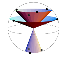
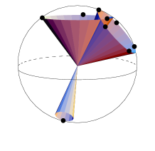
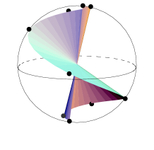
Figure 1: Examples of nested cones, free cones, and a spiral constellation for spin quantum number $s=1$. Each set of nine points defines an allowed constellation.

Random constellations

As shown in [16], almost any distribution of $N_{s}$ points on the sphere ${\sf S}^{2}$ gives rise to an allowed constellation. A random selection of directions leads with probability one to an invertible Gram matrix. This result shows that in an infinitesimal neighborhood of any forbidden constellation one can find an allowed one.

Nested cones

Historically, this family of constellations provided the first example of allowed constellations for both integer and half-integer spins [17]. For an integer value of $s$, e.g., consider $(2s+1)$ cones about one axis in space, ${\bf e}_{z}$, say, all with different opening angles. Distribute $(2s+1)$ directions over each of these nested cones in such a way that the ensemble of directions on each cone is invariant under a rotation about ${\bf e}_{z}$ by an angle $2\pi/(2s+1)$. For specific opening angles of the cones, the inversion of the matrix ${\sf N}$ in (73) reduces after a Fourier transformation to the inversion of $(2s+1)$ Vandermonde matrices of size $(2s+1)\times(2s+1)$. For a half-integer spin the same construction is possible except that the directions on different cones must also lie on different meridians. There is, in fact, a slight generalization of this result: the same calculation with $(2s+1)$ arbitrary different opening angles leads to $(2s+1)$ generalized Vandermonde matrices with nonzero determinant defining thus also a allowed constellations.

Constellations on nested cones are useful also for numerical calculations because they allow one to distribute $N_{s}$ points in a homogeneous fashion on the surface of the sphere. If two points of a constellation approach each other, the determinant of the matrix ${\sf G}$ typically becomes very large, with a disastrous effect on numerical precision.

Free cones

Here is another family of constellation involving $(2s+1)$ cones with directions located on them. However, now the cones may be oriented arbitrarily (no nesting), and the number of directions may vary from cone to cone. For example, the number of points on a cone can be chosen to equal the multiplicities of the spherical harmonics $Y_{lm}$ with $l=2s$. It is claimed that allowed constellations can be identified by taking into account the following properties (tested numerically for values up to $s=6$):

1. The determinant of ${\sf G}$ is zero if there are more than $(4s+1)$ directions on a single cone.

2. If there are $(4s+1)$ points on one cone, then another cone will contain at most $(4s-1)$ points, allowing for no more than $(4s-3)$ directions on the third cone, etc.

3. It is necessary to have directions located on at least $(2s+1)$ different cones.

For a spin $1/2$ these properties will be shown to hold in the next section. The first of these observations can be proved for arbitrary spin $s$ by using a particular decomposition of the matrix ${\sf G}$,

$${\sf G}={\sf g}^{\dagger}{\sf g}\,,$$ (79)

exploiting the fact that a positive definite matrix can always be written as the ‘square’ of its ‘root.’ A lengthy calculation involving properties of rotation matrices, Legendre polynomials and spherical harmonics leads to a factorization, ${\sf g}={\sf d}{\sf y}$, the first matrix being diagonal and having $(2s+1)$ different entries,

$${\sf d}_{(l)}=\frac{2\sqrt{\pi}(2s)!}{\sqrt{(2s+1+l)!(2s-l)!}}\,,\qquad l=0,\ldots,2s\,,$$ (80)

each value occurring $(2l+1)$ times. The second matrix has columns given by the $N_{s}$ lowest spherical harmonics evaluated at one of the $N_{s}$ points of the constellation,

$${\sf y}=\left(\begin{array}[]{cccc}Y_{00}({\bf n}_{1})&Y_{00}({\bf n}_{2})&\dots&Y_{00}({\bf n}_{N_{s}})\\ Y_{1-1}({\bf n}_{1})&Y_{1-1}({\bf n}_{2})&\dots&Y_{1-1}({\bf n}_{N_{s}})\\ \vdots&\vdots&\ddots&\vdots\\ Y_{2s2s}({\bf n}_{1})&Y_{2s2s}({\bf n}_{2})&\dots&Y_{2s2s}({\bf n}_{N_{s}})\\ \end{array}\right)\,.$$ (81)

Consequently, the Gram matrix ${\sf G}$ is invertible if and only if $\det{\sf y}\neq 0$. The matrix (81) can accomodate at most $(4s+1)$ directions on one cone, corresponding to one value of $\vartheta$ with respect to some fixed axis. The subsequent multiplicities $(4s-1),(4s-3),\ldots$, are due to applying the same argument to the remaining subspaces with dimensions $2(l-1)+1,2(l-2)+1,\ldots$

In physical terms, determinant of (81) is easily interpreted as a Slater determinant of a quantum system: it equals the (totally anti-symmetric) ground-state wave-function of $N_{s}$ non-interacting fermions restricted to move on a sphere. The node lines of this wave function correspond to forbidden constellations in which the corresponding operator kernel is degenerate, i.e., does not give rise to a basis in ${\cal A}_{s}$.

Spirals

A particularly convenient constellation is defined in the following way: let the $N_{s}$ directions be defined by $N_{s}$ complex numbers points $z_{\nu}$ constructed out of a single point $z_{0}$ (neither of modulus one nor purely real),

$$z_{\nu}=z_{0}^{\nu-1}\,,\qquad\nu=1,\ldots,N_{s}\,.$$ (82)

The points are thus located on a spiral in the complex plane.

The matrix ${\sf N}$ defined in (73) then turns into an $(N_{s}\times N_{s})$ Vandermonde matrix, that is,

$${\sf V}_{\nu\mu}=x_{\nu}^{\mu-1}\,,\qquad\nu,\mu=1,\ldots,N_{s}\,.$$ (83)

Its inverse is known explicitly (84), given, for example, in [18], with elements

$${\sf V}^{-1}_{\nu\mu}=\frac{(-1)^{\nu+1}}{\prod_{\lambda\neq\mu}(x_{\lambda}-x_{\mu})}\,S_{N_{s}-\nu}(\{x_{\lambda}\}_{\lambda=1}^{N_{s}}-x_{\mu})\,,$$ (84)

where $S_{N_{s}-\nu}(\{x_{\lambda}\}_{\lambda=1}^{N_{s}}-x_{\mu})$ is the symmetrical function constructed out of the $N-\nu$ numbers $x_{\nu}$ with $\nu\neq\lambda$. One has, for example, $S_{2}(x_{1},x_{2},x_{3})=x_{1}x_{2}+x_{1}x_{3}+x_{2}x_{3}$.

5 Discrete Moyal representation for a spin $1/2$

In this section the discrete Moyal representation will be worked out in detail for a spin with quantum number $s=1/2$, allowing for explicit results throughout. For clarity, it is assumed from the outset that the kernel consists of four projection operators

$${\widehat{Q}}_{\nu}=|{\bf n}_{\nu}\rangle\langle{\bf n}_{\nu}|\,,\qquad\nu=1,\ldots,N_{s}\,.$$ (85)

It is easy to generalize the results derived below to the case of four linear combinations of $|\pm{\bf n}_{\nu}\rangle\langle\pm{\bf n}_{\nu}|$ compatible with Eq. (12).

Let us start with the determination of the dual kernel which can be found by the intermediate step of inverting the $(4\times 4)$ Gram matrix with elements

$${\sf G}=|\langle{\bf n}_{\mu}|{\bf n}_{\nu}\rangle|^{2}=\frac{1}{2}\left(1+{\bf n}_{\mu}\cdot{\bf n}_{\nu}\right)\,.$$ (86)

This matrix is easily factorized: ${\sf G}={\sf g}^{\dagger}{\sf g}/2$, where

$${\sf g}=\left(\begin{array}[]{c c c c}1&1&1&1\\ n_{1x}&n_{2x}&n_{3x}&n_{4x}\\ n_{1y}&n_{2y}&n_{3y}&n_{4y}\\ n_{1z}&n_{2z}&n_{3z}&n_{4z}\end{array}\right).$$ (87)

The absolute value of the determinant of ${\sf g}$ is proportional to the volume of the tetrahedron defined by the four points ${\bf n}_{\nu}$ on the surface of the sphere implying $|\det{\sf G}|=18V_{tetra}$. Since a ‘flat’ tetrahedron has no volume, the entire set of forbidden constellations has a simple geometric description:

$$\det{\sf G}=0\Longleftrightarrow{\rm the~{}four~{}points~{}}{\bf n}_{\nu}~{}{\rm are~{}located~{}on~{}a~{}circle~{}on~{}}{\cal S}^{2}.$$ (88)

Consequently, allowed constellations are characterized by three vectors on a cone (any three points on a sphere define a circle), plus any fourth vector not on this cone. This agrees with the earlier statements about free-cones constellations.

Here is a simple way to invert the matrix ${\sf g}$ and subsequently ${\sf G}$. Consider a matrix

$${\sf f}=\left(\begin{array}[]{c c c c}1&{f}^{1}_{x}&{f}^{1}_{y}&{f}^{1}_{z}\\ 1&{f}^{2}_{x}&{f}^{2}_{y}&{f}^{2}_{z}\\ 1&{f}^{3}_{x}&{f}^{3}_{y}&{f}^{3}_{z}\\ 1&{f}^{4}_{x}&{f}^{4}_{y}&{f}^{4}_{z}\end{array}\right)\,,$$ (89)

defined in terms of four vectors ${\bf f}^{\nu}=(f_{x}^{\nu},f_{y}^{\nu},f_{z}^{\nu})$ not required to have length one. The matrix elements of the of product ${\sf f}$ and ${\sf g}$ are given by

$$\left({\sf f}{\sf g}\right)^{\mu}_{\nu}=1+{\bf f}^{\mu}\cdot{\bf n}_{\nu}\,.$$ (90)

This is a diagonal matrix if the scalar products ${\bf f}^{\mu}\cdot{\bf n}_{\mu}$ equal $-1$ whenever $\mu\neq\nu$. Geometrically, such four vectors are constructed easily: the vector ${\bf f}^{1}$ points to the unique intersection of the three planes tangent to the sphere at the points $-{\bf n}_{2}$, $-{\bf n}_{3}$ and $-{\bf n}_{4}$. Analytically, this vector reads

$${\bf f}^{1}=\frac{{\bf n}_{2}\wedge{\bf n}_{3}+{\bf n}_{3}\wedge{\bf n}_{4}+{\bf n}_{4}\wedge{\bf n}_{2}}{({\bf n}_{2}\wedge{\bf n}_{3})\cdot{\bf n}_{4}}\,,$$ (91)

and the three remaining vectors follow from cyclic permutation of the numbers $1$ to $4$. With this choice the inverse of the matrix ${\sf g}$ can be written as

$${\sf g}^{-1}={\sf d}^{-1}{\sf f}\,,$$ (92)

where ${\sf d}$ is the diagonal matrix in (90): ${\sf d}_{\nu\nu}=1+{\bf f}^{\nu}\cdot{\bf n}_{\nu}$. Consequently, the inverse of the Gram matrix ${\sf G}$ for a general allowed constellation is given by

$${\sf G}^{-1}=2\,{\sf d}^{-1}{\sf f}\,{\sf f}^{\dagger}{\sf d}^{-1}\,,$$ (93)

having matrix elements

$${\sf G}^{-1}_{\mu\nu}\equiv{\sf G}^{\mu\nu}=2\,\frac{1+{\bf f}^{\mu}\cdot{\bf f}^{\nu}}{(1+{\bf n}_{\mu}\cdot{\bf f}^{\mu})(1+{\bf n}_{\nu}\cdot{\bf f}^{\nu})}\,.$$ (94)

In general, the elements ${\widehat{Q}}^{\nu}$ of the dual kernel will thus be linear combinations of all four projection operators ${\widehat{Q}}_{\nu}$.

It is interesting to express the kernel and its dual in terms of the Pauli matrices $\sigma\sigma=(\sigma_{x},\sigma_{y},\sigma_{z})$:

$${\widehat{Q}}_{\nu}=\frac{1}{2}({\sf I}+{\bf n}_{\nu}\cdot\sigma\sigma)\,,\qquad{\widehat{Q}}^{\nu}=2\,\frac{{\sf I}+{\bf f}^{\nu}\cdot\sigma\sigma}{1+{\bf f}^{\nu}\cdot{\bf n}_{\nu}}\,,$$ (95)

allowing one to show easily that they satisfy the required duality.

For reference, we give the $Q$- and $P$-symbols of the spin operator

$${\bf s}_{\nu}=\frac{1}{2}{\bf n}_{\nu}\,,\qquad{\bf s}^{\nu}=\frac{2\,{\bf f}^{\nu}}{1+{\bf f}^{\nu}\cdot{\bf n}_{\nu}}\,,$$ (96)

and of the identity,

$$I_{\nu}=1\,,\qquad I^{\nu}=\frac{4}{1+{\bf f}^{\nu}\cdot{\bf n}_{\nu}}\,,$$ (97)

and the symbols of arbitrary operators for a spin $1/2$ follow from linear combinations.

6 Discussion

Operator kernels have been used for a systematic study of phase-space representations of a quantum spin $s$. The kernels have been derived from appropriate Stratonovich-Weyl postulates taking slightly different forms for continuous and discrete representations, respectively. Emphasis is on the discrete Moyal formalism which allows one to describe hermitean operators, including density matrices, by a minimal number of probabilities easily measured by a Stern-Gerlach apparatus. As a useful by-product a natural and most economic method of state reconstruction emerges when a quantum spin is described in terms of discrete symbols. Further, Schrödinger’s equation for a spin $s$ turns into a set of coupled linear differential equations for $(2s+1)^{2}$ probabilities [19].

In addition, a new form of the kernel defining continuous Wigner functions for a spin has been obtained (20): it has been expressed as an ensemble of operators obtained from all possible rotations of one fixed operator. This is entirely analogous to an elegant expression of the kernel for particle-Wigner functions as the ensemble of all possible phase-space translations of the parity operator. Therefore, continuous phase-space representations for both spin and particle systems now are seen to derive from structurally equivalent operator kernels.

The discrete symbolic calculus is an interesting ‘hybrid’ between the classical and quantal descriptions of a spin. On the one hand, this representation is equivalent to standard quantum mechanics of a spin. On the other, the independent variables carry phase-space coordinates as labels (51,52). However, only a finite subset of points in phase space (corresponding to an allowed constellation) are involved reflecting thus the discretization characteristic of quantum mechanics.

The $N_{s}$ projections operators associated with a constellation of points define a non-orthogonal basis for hermitean operators acting on the Hilbert space of the spin. Each projection is a positive operator, and, altogether, they give rise to a resolution of unity. One might suspect that they define a positive operator-valued measure [20] or POVM, for short. However, this is not the case since the closure relation does not involve just the bare projections but they are multiplied with factors some of which necessarily take negative values. Such an obstruction through ‘negative probabilities’ is not surprising; other phase-space representations are based on quantum mechanical ‘quasi-probabilities,’ known to have this property, too.

Let us close with a synopsis of the fundamental Moyal-type representations for particle and spin systems known so far.

	self-dual kernel	dual pairs
particle	Wigner functions [ unknown ]	$P$-, $Q$-symbols [ unknown ]
spin	Stratonovich/Varilly [ impossible ]	Berezin symbols [ $P^{\nu}$-, $Q_{\nu}$-symbols]

The table provides both a summary and points at open questions. The individual entries give the names of the familiar continuous phase-space representations while the corresponding quantities for the discrete formalism are in square brackets. Future work will focus on developing a discrete Moyal-type formalism for a quantum particle. To do this, one must exhibit, for example, a pair of dual kernels one of which would consist of a countable set of projection operators on coherent states. This set is required to be a basis in the linear space of (bounded?) operators on the particle Hilbert-space. It is not obvious in which way the associate discrete $P$-symbol would reflect the subtleties of its continuous counterpart which may be singular. Similarly, the existence of a self-dual discrete kernel for a quantum particle is an open question.

Acknowledgements

St. W. acknowledges financial support by the Schweizerische Nationalfonds.

References

- [1] E. P. Wigner: Phys. Rev. 40 (1932) 749.
- [2] J. E. Moyal: Proc. Cambridge Philos. Soc. 45 (1949) 99.
- [3] A. Royer: Phys. Rev. A 15 (1977) 449.
- [4] P. Huguenin and J.-P. Amiet: Mécaniques classique et quantique dans l’espace de phase. Université de Neuchâtel, Neuchâtel, 1981.
- [5] A. Perelomov: Generalized Coherent States and their Applications., Springer Verlag, Berlin, 1986.
- [6] R. L. Stratonovich: JETP 4 (1957) 891.
- [7] J. Várilly and J.M. Gracia-Bondía: Ann. Phys. 190 (1989) 107.
- [8] J.-P. Amiet and M. B. Cibils: J. Phys. A: Math. Gen. 24 (1991) 1515 .
- [9] F. A. Berezin: Commun. Math. Phys. 40 (1975) 153.
- [10] J.-P. Amiet and St. Weigert: J. Phys. A: Math. Gen. 31 (1998) L543.
- [11] St. Weigert: Reconstruction of Spin States and its Conceptual Implications. I n: New Insights in Quantum Mechanics, H.-D. Doebner, S. T. Ali, M. Keyl, and R. F. Werner (eds.) World Scientific (in press) (=quant-ph/9809065).
- [12] F.T. Arecchi, E. Courtens, R. Gilmore, and H. Thomas: Phys. Rev. A 6 (1972) 2211.
- [13] A.R. Edmonds: Angular Momentum in Quantum Mechanics, Princeton University Press, 1957.
- [14] J.-P. Amiet and St. Weigert: Contraction of Spin Wigner-Functions to Particle Wigner-Functions (unpublished).
- [15] W. H. Greub: Linear Algebra, Springer, Berlin, 1963.
- [16] J.-P. Amiet and St. Weigert: J. Opt. B, (in press) (=quant-ph/9906099).
- [17] J.-P. Amiet and St. Weigert: J. Phys. A: Math. Gen. 32 (1999) 269 (=quant-ph/9903067).
- [18] L. Verde-Star: J. Math. Anal. Appl. 131 (1988) 341.
- [19] St. Weigert: Phys. Rev. Lett. 84 (2000) 802 (=quant-ph/99030103)
- [20] J. M. Jauch and C. M. Piron: Helv. Phys. Acta 40 (1967) 559.