Entanglement transformation at absorbing and amplifying four-port devices

Abstract

Dielectric four-port devices play an important role in optical quantum information processing. Since for causality reasons the permittivity is a complex function of frequency, dielectrics are typical examples of noisy quantum channels, which cannot preserve quantum coherence. To study the effects of quantum decoherence, we start from the quantized electromagnetic field in an arbitrary Kramers–Kronig dielectric of given complex permittivity and construct the transformation relating the output quantum state to the input quantum state, without placing restrictions on the frequency. We apply the formalism to some typical examples in quantum communication. In particular we show that for Fock-entangled qubits the Bell-basis states $|\Psi^{\pm}\rangle$ are more robust against decoherence than the states $|\Phi^{\pm}\rangle$.

I Introduction

Quantum communication schemes widely use dielectric four-port devices as basic elements for constructing optical quantum channels. A typical example of such a device is a beam splitter as a basic element not only for classical interference experiments but also for implementing quantum interferences. Another example is an optical fiber, which can be regarded as a dielectric four-port device that essentially realizes transmission of light over longer distances.

Dielectric matter is commonly described in terms of the (spatially varying) permittivity as a complex function of frequency, whose real and imaginary parts are related to each other by the Kramers–Kronig relations. Since the appearance of the imaginary part (responsible for absorption and/or amplification) is unavoidably associated with additional noise, dielectric devices are typical examples of noisy quantum channels. Using them for generating or processing entangled quantum states of light, e.g., in quantum teleportation or quantum cryptography, the question of quantum decoherence arises.

In order to study the problem, quantization of the electromagnetic field in the presence of dielectric media is needed. For absorbing bulk material, a consistent formalism is given in [1], using the Hopfield model of a dielectric [2]. A method of direct quantization of Maxwell’s equations with a phenomenologically introduced permittivity is given in [3]. It replaces the familiar mode decomposition of the electromagnetic field with a source-quantity representation, expressing the field in terms of the classical Green function and the fundamental variables of the composed system. The method has the benefit of being independent of microscopic models of the medium and can be extended to arbitrary inhomogeneous dielectrics [4, 5]. All relevant information about the medium are contained in the permittivity (and the resulting Green function), and quantization is performed by the association of bosonic quantum excitations with the fundamental variables.

Quantization of the phenomenological Maxwell field is especially well suited for deriving the input-output relations of the field [6, 7, 8, 9] on the basis of the really observed transmission and absorption coefficients. In particular, there is no need to introduce artificial replacement schemes. Applications to low-order correlations in two-photon interference effects have been given [8, 10, 11].

The formalism has also been extended to amplifying media [5, 12]. The resulting input–output relations for amplifying beam splitters have been used to compute first- and second-order moments of photo counts [13] and normally ordered Poynting vectors [14]. Further, propagation of squeezed radiation through amplifying or absorbing multiport devices has been considered [15].

For the study of entanglement, however, knowledge of some moments and correlations is not enough. In particular, to answer the question as to whether or not a bipartite quantum state is separable and to calculate the degree of entanglement of a nonseparable state, the complete information on the state is required in general.

Recently we have presented closed formulas for calculating the output quantum state from the input quantum state [16], using the input–output relations for the field at an absorbing four-port device of given complex refractive-index profile. In this paper we apply these results to study the entanglement properties influenced by propagation in real dielectrics and extend the theory also to amplifying four-port devices. Enlarging the system by introducing appropriately chosen auxiliary degrees of freedom, we first construct the unitary transformation in the enlarged Hilbert space. Taking the trace with regard to the auxiliary variables, we then obtain the sought formulas for the transformation of arbitrary input quantum states. Finally, we discuss some applications, with special emphasis on the dependence of entanglement on absorption and amplification.

The paper is organized as follows. In Sec. II the basic equations are reviewed and the general transformation formulas are derived. Examples of possible applications are discussed in Sec. III, and some conclusions are given in Sec. IV.

II Quantum state transformations

A Basic equations

Let us briefly review some basic formulas needed for the following calculations. For simplicity, we restrict ourselves to a quasi-one-dimensional scheme (Fig. 1). The action of the dielectric device on the incoming radiation is described by means of the characteristic $2$ $\!\times$ $\!2$ transformation and absorption matrices ${\bf T}(\omega)$ and ${\bf A}(\omega)$ respectively, which are derived in [8] on the basis of the quantization scheme in [3]. They are given in terms of the complex refractive-index profile $n(x,\omega)$ of the device. Let $\hat{a}_{i}(\omega)$ and $\hat{b}_{i}(\omega)$, $i$ $\!=$ $\!1,2$, be the amplitude operators of the incoming and outgoing damped waves at frequency $\omega$. Taking their spatial arguments at the boundary of the device, we may regard them as being effectively bosonic operators [8]. Further, let $\hat{g}_{i}(\omega)$ be the bosonic operators of the device excitations, which play the role of operator noise forces associated with absorption or amplification. Introducing the two-vector notation $\hat{\bf a}(\omega)$, $\hat{\bf b}(\omega)$ and $\hat{\bf g}(\omega)$, for the field and device operators respectively, we may write the input-output relation for radiation at an absorbing or amplifying device in the compact form

$$\hat{\bf b}(\omega)={\bf T}(\omega)\hat{\bf a}(\omega)+{\bf A}(\omega)\hat{\bf d}(\omega),$$ (1)

where the transformation and absorption matrices satisfy the relation

$${\bf T}(\omega){\bf T}^{+}(\omega)+\sigma{\bf A}(\omega){\bf A}^{+}(\omega)={\bf I},$$ (2)

and $\sigma$ $\!=$ $\!+1$, $\hat{\bf d}(\omega)$ $\!=$ $\!\hat{\bf g}(\omega)$ for absorbing devices and $\sigma$ $\!=$ $\!-1$, $\hat{\bf d}(\omega)$ $\!=$ $\!\hat{\bf g}^{\dagger}(\omega)$ for amplifying devices. The above given equations are valid for any chosen frequency. Knowing the amplitude operators as functions of frequency, the full-field operators can be constructed by appropriate integration over the frequency in a straightforward way [8].

B Unitary operator transformations

The operator input-output relation (1) contains all the information necessary to transform an arbitrary function of the input-field operators into the corresponding function of the output-field operators. In particular, it enables one to express arbitrary moments and correlations of the outgoing field in terms of those of the incoming field and the device excitations, and hence all knowable information about the quantum state of the outgoing field can be obtained. Commonly, quantum states are expressed in terms of density matrices or phase-space functions – representations that are more suited to study a quantum state as a whole.

In order to calculate the density operator of the outgoing field for both absorbing and amplifying devices, we follow the line given in [16] for absorbing devices. We first define the four-vector operators

$$\hat{\mbox{\boldmath$\alpha$}}(\omega)=\left(\begin{array}[]{c}\hat{\bf a}(\omega)\\ \hat{\bf d}(\omega)\end{array}\right)\,,\quad\hat{\mbox{\boldmath$\beta$}}(\omega)=\left(\begin{array}[]{c}\hat{\bf b}(\omega)\\ \hat{\bf f}(\omega)\end{array}\right),$$ (3)

where $\hat{\bf f}(\omega)$ $\!=$ $\!\hat{\bf h}(\omega)$ for an absorbing device, and $\hat{\bf f}(\omega)$ $\!=$ $\!\hat{\bf h}^{\dagger}(\omega)$ for an amplifying device, with $\hat{\bf h}(\omega)$ being some auxiliary bosonic (two-vector) operator. The input-output relation (2) can then be extended to the four-dimensional transformation

$$\hat{\mbox{\boldmath$\beta$}}(\omega)=\mbox{\boldmath$\Lambda$}(\omega)\hat{\mbox{\boldmath$\alpha$}}(\omega)$$ (4)

with

$$\mbox{\boldmath$\Lambda$}(\omega)\mbox{\boldmath$J$}\mbox{\boldmath$\Lambda$}^{+}(\omega)=\mbox{\boldmath$J$},\qquad\mbox{\boldmath$J$}=\left(\begin{array}[]{cc}{\bf I}&{\bf 0}\\ {\bf 0}&\sigma{\bf I}\end{array}\right).$$ (5)

Hence, $\mbox{\boldmath$\Lambda$}(\omega)$ $\!\in$ SU($4$) for absorbing devices [16], and $\mbox{\boldmath$\Lambda$}(\omega)$ $\!\in$ SU($2,2$) for amplifying devices (if an overall phase factor is included in the input operators). Note, that lossless devices, where ${\bf A}(\omega)$ $\!\equiv$ $\!{\bf 0}$, can be described by SU($2$) group transformations [17, 18]. Since the group SU($4$) is compact, while SU($2,2$) is noncompact, qualitatively different properties of the state transformations are expected to occur in these two cases. Introducing the (commuting) positive Hermitian matrices

$${\bf C}(\omega)=\sqrt{{\bf T}(\omega){\bf T}^{+}(\omega)},\quad{\bf S}(\omega)=\sqrt{{\bf A}(\omega){\bf A}^{+}(\omega)},$$ (6)

which, by Eq. (2), obey the relation ${\bf C}^{2}(\omega)$ $\!+$ $\!\sigma{\bf S}^{2}(\omega)$ $\!=$ $\!{\bf I}$, it is not difficult to generalize the matrix $\mbox{\boldmath$\Lambda$}(\omega)$ in [16] to

$$\mbox{\boldmath$\Lambda$}(\omega)=\left(\begin{array}[]{cc}{\bf T}(\omega)&{\bf A}(\omega)\\ -\sigma{\bf S}(\omega){\bf C}^{-1}(\omega){\bf T}(\omega)&{\bf C}(\omega){\bf S}^{-1}(\omega){\bf A}(\omega)\end{array}\right).$$ (7)

Both the SU($4$) and SU($2,2$) group elements can be written in exponential form

$$\mbox{\boldmath$\Lambda$}(\omega)={\rm e}^{-i\mbox{\boldmath$\Phi$}(\omega)}\,,\quad\mbox{\boldmath$\Phi$}^{+}(\omega)=\mbox{\boldmath$J$}\mbox{\boldmath$\Phi$}(\omega)\mbox{\boldmath$J$},$$ (8)

and a unitary operator transformation

$$\hat{\mbox{\boldmath$\beta$}}(\omega)=\hat{U}^{\dagger}\hat{\mbox{\boldmath$\alpha$}}(\omega)\hat{U}$$ (9)

can be constructed, where

$$\hat{U}={\rm exp}\Bigg{\{}-i\int_{0}^{\infty}d\omega\left[\hat{\mbox{\boldmath$\alpha$}}^{\dagger}(\omega)\right]^{T}\mbox{\boldmath$J$}\mbox{\boldmath$\Phi$}(\omega)\hat{\mbox{\boldmath$\alpha$}}(\omega)\Bigg{\}}.$$ (10)

Note that the unitarity of $\hat{U}$ follows directly from Eq. (8).

Let the density operator of the input quantum state be a functional of $\hat{\mbox{\boldmath$\alpha$}}(\omega)$ and $\hat{\mbox{\boldmath$\alpha$}}^{\dagger}(\omega)$, $\hat{\varrho}_{\rm in}$ $\!=$ $\!\hat{\varrho}_{\rm in}[\hat{\mbox{\boldmath$\alpha$}}(\omega),\hat{\mbox{\boldmath$\alpha$}}^{\dagger}(\omega)]$. The density operator of the quantum state of the outgoing fields can then be given by

$$\hat{\varrho}^{(F)}_{\rm out}={\rm Tr}^{(D)}\left\{\hat{U}\hat{\varrho}_{\rm in}\hat{U}^{\dagger}\right\}$$ (12)

$$={\rm Tr}^{(D)}\left\{\hat{\varrho}_{\rm in}\left[\mbox{\boldmath$J$}\mbox{\boldmath$\Lambda$}^{+}(\omega)\mbox{\boldmath$J$}\hat{\mbox{\boldmath$\alpha$}}(\omega),\mbox{\boldmath$J$}\mbox{\boldmath$\Lambda$}^{T}(\omega)\mbox{\boldmath$J$}\hat{\mbox{\boldmath$\alpha$}}^{\dagger}(\omega)\right]\right\},$$

where ${\rm Tr}^{(D)}$ means trace with respect to the device variables. It should be pointed out that $\hat{\varrho}^{(F)}_{\rm out}$ in Eq. (12) does not depend on the auxiliary variables introduced in Eq. (4). The SU(4)-group transformation preserves operator ordering and thus for absorbing devices, the $s$-parametrized phase-space functions transform as

$$P_{\rm out}[\mbox{\boldmath$\alpha$}(\omega);s]=P_{\rm in}[\mbox{\boldmath$\Lambda$}^{+}(\omega)\mbox{\boldmath$\alpha$}(\omega);s].$$ (13)

Since the SU(2,2)-group transformation mixes creation and annihilation operators, an equation of the type (13) is not valid for amplifying devices in general. An exception is the Wigner function that corresponds to symmetrical ordering ($s$ $\!=$ $\!0$):

$$W_{\rm out}\left[\mbox{\boldmath$\alpha$}(\omega)\right]=W_{\rm in}[\mbox{\boldmath$J$}\mbox{\boldmath$\Lambda$}^{+}(\omega)\mbox{\boldmath$J$}\mbox{\boldmath$\alpha$}(\omega)].$$ (14)

For amplifying devices, the calculation of the output state is rather involved in general. Formulas for Fock-state transformation are given in the Appendix.

III Applications

As already mentioned, the input-output relation (1) enables one to calculate arbitrary moments and correlations of the outgoing field. It is worth noting that there is no need to introduce fictitious beam splitters for modeling the losses. The transmittance and absorption matrices in Eq. (1) automatically take account of the losses, because they are calculated from Maxwell’s equations with complex permittivity. To give an example, we compute in Sec. III A the visibility of interference fringes in photon-number detection in a Mach-Zehnder interferometer with lossy beam splitters.

The input-output relation (12) can advantageously be used when knowledge of the transformed quantum state as a whole is required. This is typically the case in quantum communication, which is essentially based on entangled quantum states. For quantification of entanglement – a quantum-coherence property that sensitively responds to losses – information about the full quantum state is needed in general. The entanglement measure we use is the quantum relative entropy (the quantum analog of the classical Kullback–Leibler entropy) defined by [19]

$$E(\hat{\sigma})=\min_{\hat{\rho}\in{\cal S}}{\rm Tr}\left[\hat{\sigma}\left(\ln\hat{\sigma}-\ln\hat{\rho}\right)\right],$$ (15)

with $\hat{\sigma}$ and ${\cal S}$ being, respectively, the bipartite quantum state under study and the set of all separable quantum states. We stress here that the relative entropy is indeed a “good” entanglement measure, because it satisfies the necessary conditions that should be required of such a measure [19, 20, 21]. Note that any proper entanglement measure satisfying them would do (the Bures metric being another typical example).

In Sec. III B we study the entanglement produced at a realistic beam splitter by initially uncorrelated photons, and in Sec. III C we analyze the degradation of entanglement during propagation through lossy media, with special emphasis on Bell-type states. Effects associated with amplification are addressed in Sec. III D.

A Visibility of interference fringes

To give an example of application of the input-output relations (1), we consider the visibility of interference fringes in a Mach–Zehnder interferometer in Fig. 2. A single photon is fed into one input port, the other input port being unused. The quantity we are interested in is the visibility

$$V_{k}=\frac{\langle\hat{n}_{k}\rangle_{\rm max}-\langle\hat{n}_{k}\rangle_{\rm min}}{\langle\hat{n}_{k}\rangle_{\rm max}+\langle\hat{n}_{k}\rangle_{\rm min}}\,,$$ (16)

where $\langle\hat{n}_{k}\rangle_{\rm max}$ ($\langle\hat{n}_{k}\rangle_{\rm min}$) is the maximum (minimum) value of the mean photon number in the $k$th output channel ($k$ $\!=$ $\!1,2$).

In order to model the losses in the interferometer arms (e.g., nonperfect mirrors or dissipation processes in optical fibers connecting the beam splitters BS1 and BS2), in [22] a fictitious (nonabsorbing) beam splitter is inserted into each branch of the interferometer. In practice, however, the beam splitters BS1 and BS2 are also expected to give rise to some losses. Whereas the losses arising from the beam splitter BS1 may be thought of as being included in the replacement scheme considered in [22], inclusion in the calculation of the losses arising from the beam splitter BS1 would require that two additional fictitious beam splitters were inserted between the beam splitter BS2 and the detectors. Altogether, a replacement scheme with four fictitious beam splitters at least must be considered in order to model all the losses.

Application of the input-output relations (1) shows that there is no need for such an involved replacement scheme. Instead, the proper transmittance and reflection coefficients of the beam splitters and mirrors (or fibers) can be used to obtain the correct physics, including the losses. Applying the input-output relations (1) successively to the beam splitter BS2, the lossy branches, and the beam splitter BS1 and assuming the devices are in the vacuum state, so that the overall input state is $|\psi_{\rm in}\rangle$ $\!=$ $\!|1,0,0,0\rangle$, it is not difficult to show that

$$\langle\hat{n}_{1}\rangle = |R_{1}|^{2}|T_{3}|^{2}|R_{2}|^{2}+|T_{1}|^{2}|T_{4}|^{2}|T_{2}|^{2}$$ (18)

$$+2|R_{1}||R_{2}||T_{1}||T_{2}||T_{3}||T_{4}|\cos\Theta_{1}\,,$$

$$\langle\hat{n}_{2}\rangle = |R_{1}|^{2}|T_{3}|^{2}|T_{2}|^{2}+|R_{2}|^{2}|T_{4}|^{2}|T_{1}|^{2}$$ (20)

$$+2|R_{1}||R_{2}||T_{1}||T_{2}||T_{3}||T_{4}|\cos\Theta_{2}\,,$$

where $\Theta_{1}$ $\!=$ $\!\Theta$ $\!+$ $\!\varphi_{R_{1}}$ $\!-$ $\!\varphi_{T_{1}}$ $\!+$ $\!\varphi_{R_{2}}$ $\!-$ $\!\varphi_{T_{2}}$ $\!+$ $\!\varphi_{T_{3}}$ $\!-$ $\!\varphi_{T_{4}}$ and $\Theta_{2}$ $\!=$ $\!\Theta$ $\!+$ $\!\varphi_{R_{1}}$ $\!-$ $\!\varphi_{T_{1}}$ $\!-$ $\!\varphi_{R_{2}}$ $\!+$ $\!\varphi_{T_{2}}$ $\!+$ $\!\varphi_{T_{3}}$ $\!-$ $\!\varphi_{T_{4}}$. Here and in the following, the notation $(T_{l})_{11}$ $\!=$ $\!(T_{l})_{22}$ $\!\equiv$ $\!R_{l}$ $\!=$ $\!|R_{l}|e^{i\varphi_{R_{l}}}$ and $(T_{l})_{12}$ $\!=$ $\!(T_{l})_{21}$ $\!\equiv$ $\!T_{l}$ $\!=$ $\!|T_{l}|e^{i\varphi_{T_{l}}}$ for the elements of the transmittance matrix $T$_l of the $l$th four-port device is used [$l$ $\!=$ $\!1,2$, beam splitters BS1 and BS2; $l$ $\!=$ $\!3,4$, upper (3) and lower (4) branch of the interferometer]. Note that for a lossy device

$$\arg R_{l}-\arg T_{l}\neq\pi/2$$ (21)

in general. Combining Eqs. (16) – (20), we easily derive

$$V_{1} = 2\left(\frac{|R_{1}||T_{3}||R_{2}|}{|T_{1}||T_{4}||T_{2}|}+\frac{|T_{1}||T_{4}||T_{2}|}{|R_{1}||T_{3}||R_{2}|}\right)^{-1},$$ (22)

$$V_{2} = 2\left(\frac{|R_{1}||T_{3}||T_{2}|}{|R_{2}||T_{1}||T_{4}|}+\frac{|R_{2}||T_{1}||T_{4}|}{|R_{1}||T_{3}||T_{2}|}\right)^{-1}\,.$$ (23)

It is worth noting that Eqs. (22) and (23) are valid for the really observed reflection and transmission coefficients $R_{k}$ and $T_{k}$, respectively, with

$$|R_{k}|^{2}+|T_{k}|^{2}\leq 1.$$ (24)

The equality sign would be realized for nonabsorbing devices.

Comparing with the formulas for the visibilities derived in [22], we observe that they look like Eqs. (22) and (23). However, this resemblance is only formal. In fact, all the reflection and transmission coefficients (including the phases) introduced in [22] satisfy the relations valid for nonabsorbing devices and therefore differ from the measured reflection and transmission coefficients that in a real experiment determine the fringe visibilities. Even if additional fictitious beam splitters were included in the model in [22], there would be no unique relation between auxiliary and actual parameters in general.

B Photon entanglement at a beam splitter

Superimposing two nonclassically excited modes by a lossless beam splitter, one can generate entangled states with interesting properties [17]. Two of the simplest examples are as follows. Having a single-photon Fock state in one input channel of a 50%-50% beam splitter, i.e., $|T|^{2}$ $\!=$ $\!|R|^{2}$ $\!=$ $\!1/2$, whereas the other input channel is unused, the output state is a superposition of states with the photon in one of the output channels. If each of the two incoming modes is prepared in a single-photon Fock state, then the output state is a superposition of states with two photons in one output channel. In either case, the output state is a superposition of two states and the maximum entanglement of $\ln 2$ (which corresponds to $1$ bit) is realized. Note that for pure states the entanglement measure (15) reduces to the von Neumann entropy of one subsystem. When $|T|^{2}$ $\!\neq$ $\!|R|^{2}$ then the output state in the latter case is a superposition of three states, because each outgoing mode can now contain either zero, one, or two photons. The maximum entanglement of a three-state system is $\ln 3$, which is realized if $|T|^{2}$ $\!=$ $\!1/2$ $\!\times$ $\!(\!1$ $\!\pm$ $\!1/\sqrt{3})$ (see Fig. 3). Hence, a non-50%-50% beam splitter can produce stronger entanglement than a 50%-50% beam splitter which suppresses one possible outcome owing to interference. With regard to entanglement, this interference effect is thus destructive.

Let us now raise the question of the amount of entanglement achievable in case of a realistic beam splitter – a question that may be important for the quality of quantum communication by means of entangled photonic states obtained by available devices. The question can be answered by applying the input-output relation (12) and calculating the output state of the interfering modes obtained by an absorbing beam splitter. To give an example, let us study the entanglement produced by a dielectric plate of permittivity

$$\epsilon(\omega)=1+\frac{\epsilon_{s}-1}{1-(\omega/\omega_{0})^{2}-2i\gamma\omega/\omega_{0}^{2}}$$ (25)

($\epsilon_{s}$ $\!=$ $\!1.5$) and thickness $d$ $\!=$ $\!2c/\omega_{0}$ for the case where either one or each of the two incoming modes is prepared in a single-photon Fock state. The squares of the absolute values of the calculated reflection, transmission, and absorption coefficients as functions of frequency [8] are shown in Fig. 4 for $\gamma$ $\!=$ $\!0.001$. When the device is not excited, then the overall input state is either $|1,0,0,0\rangle$ or $|1,1,0,0\rangle$ for the two cases under consideration. The resulting mixed states of the outgoing modes are calculated in [16]. Here, we have calculated the amount of entanglement of the states using the definition (15).

Results are plotted in Figs. 5 and 6 for $\gamma$ $\!=$ $\!0.001$, and in Fig. 7 for $\gamma$ $\!=$ $\!0.01$. For comparison, the figures also show the mutual information $I_{c}$ $\!=$ $\!S_{1}$ $\!+$ $\!S_{2}$ $\!-$ $\!S_{12}$, where $S_{1}$ and $S_{2}$ are the von Neumann entropies of the outgoing modes $1$ and $2$, respectively, and $S_{12}$ is the entropy of the composite two-mode system. Obviously, the mutual information may be regarded as a measure of the total amount of correlation contained in the states. In regions where the absorption is sufficiently weak, the output state is almost pure, and thus $S_{12}$ $\!\approx$ $\!0$ and $E(\hat{\sigma})$ $\!\approx$ $\!S_{i}$. Hence, the two curves in Figs. 5 and 6 differ there only by a factor approximately equal to two. With increasing absorption the two curves cannot be related to each other by simple scaling, as it can be seen from Fig. 7. In particular, the maximally achievable amount of entanglement of about $0.4$ is much less than $\ln 2$ achievable with a lossless device.

From Figs. 5 and 6 strong reduction of entanglement is observed in the resonance region. Here reflection and absorption are strongest, so that the two modes are only weakly mixed and absorption prevents the device from creating quantum coherence. As expected, substantial entanglement is observed in regions where the absorption is weak and $|T|^{2}$ and $|R|^{2}$ nearly satisfy the condition of maximum entanglement. In Fig. 5 this is the case for $\omega/\omega_{0}$ $\!\approx$ $\!1.25$ where the value of entanglement becomes close to the maximally achievable value of $\ln 2$. In Fig. 6 the value of entanglement becomes close to the maximally achievable value of $\ln 3$ at $\omega/\omega_{0}$ $\!\approx$ $\!1.18$ and $\omega/\omega_{0}$ $\!\approx$ $\!1.33$. The relative minimum in Fig. 6 at $\omega/\omega_{0}$ $\!\approx$ $\!1.25$ indicates the effect of destructive interference mentioned above.

The results show that entanglement sensitively depends on the optical properties of the material used for manufacturing the optical device. They demonstrate the importance of optimizing the frequency regime of quantum communication schemes with given devices.

C Entangled-state transmission through a lossy channel

1 Bell-type basis states $|\Psi_{n}^{\pm}\rangle$

Let us now turn to the question of entanglement degradation during the propagation through dielectric matter such as an optical fiber. For this purpose, we consider two modes each of which propagates through a dielectric medium of complex permittivity. Assuming the incoming modes are prepared in a maximally entangled Bell-type state

$$|\Psi_{n}^{\pm}\rangle=\frac{1}{\sqrt{2}}\left(|0n\rangle\pm|n0\rangle\right),$$ (26)

we apply Eq. (12) and calculate the quantum state of the two outgoing modes. After some algebra we derive

$$\hat{\varrho}_{\rm out}^{({\rm F})} = \frac{1}{2}\Bigg{[}\sum\limits_{k=0}^{n-1}{n\choose k}|T_{1}|^{2k}\left(1-|T_{1}|^{2}\right)^{n-k}|k0\rangle\langle k0|$$ (29)

$$\hskip 8.61108pt+\sum\limits_{k=0}^{n-1}{n\choose k}|T_{2}|^{2k}\left(1-|T_{2}|^{2}\right)^{n-k}|0k\rangle\langle 0k|\Bigg{]}$$

$$\hskip 8.61108pt+{\textstyle\frac{1}{2}}\left(|T_{1}|^{2n}+|T_{2}|^{2n}\right)\,|\Psi^{\prime}_{n}{{}^{\!\pm}}\rangle\langle\Psi^{\prime}_{n}{{}^{\!\pm}}|,$$

where

$$|\Psi^{\prime}_{n}{{}^{\!\pm}}\rangle=\left(|T_{1}|^{2n}\!+\!|T_{2}|^{2n}\right)^{-1/2}\big{(}T_{1}^{n}|n0\rangle\pm T_{2}^{n}|0n\rangle\big{)}.$$ (30)

Note that when setting $n$ $\!=$ $\!1$, the transformation of the ordinary Bell basis states $|\Psi^{\pm}\rangle$ $\!\equiv$ $\!|\Psi_{1}^{\pm}\rangle$ are obtained. In what follows we assume that the transmission coefficients $T_{k}$ ($k$ $\!=$ $\!1,2$) are given by

$$T_{k}=T_{k}(\omega)={\rm e}^{in_{k}(\omega)\omega l_{k}/c},$$ (31)

with $n_{k}(\omega)$ $\!=$ $\!\sqrt{\epsilon_{k}(\omega)}$ $\!=$ $\eta_{k}(\omega)+i\kappa_{k}(\omega)$ and $l_{k}$ being the complex refractive indexes of the media and the propagation lengths, respectively. According to the Lambert–Beer law, $|T_{k}|$ decreases exponentially with the length of propagation: $|T_{k}|$ $\!=$ $\!\exp(-l_{k}/L_{k})$, $L_{k}$ $\!=$ $\!c/(\omega\kappa_{k})$. In special cases when one mode propagates through vacuum, $n(\omega)$ $\!=$ $\!1$, the corresponding transmission coefficient, by Eq. (31), is just a phase factor.

For a first insight into the behavior of the transmitted quantum state it may be instructive to look at the overlap of the output state with the input state, which is

$$\langle\Psi_{n}^{\pm}|\hat{\varrho}_{\rm out}^{({\rm F})}|\Psi_{n}^{\pm}\rangle={\textstyle\frac{1}{4}}\left(|T_{1}|^{2n}\!+\!|T_{2}|^{2n}\!+\!T_{1}^{\ast n}T_{2}^{n}\!+\!T_{1}^{n}T_{2}^{\ast n}\right).$$ (32)

We see that the characteristic length of degradation of the overlap (fidelity) is not given by $L_{k}$ but by the shorter length $L_{k}/(2n)$. Hence, the overlap rapidly approaches zero with increasing number of photons even for weak damping of the intensity or related (classical) quantities.

As already mentioned, a proper measure of entanglement is the quantum relative entropy defined by Eq. (15). In order to estimate an upper bound, we employ the convexity property [23]

$$E[\lambda\hat{\sigma}_{1}+(1-\lambda)\hat{\sigma}_{2}]\leq\lambda E(\hat{\sigma}_{1})+(1-\lambda)E(\hat{\sigma}_{2})\,.$$ (33)

From Eq. (29) it is seen that $\hat{\varrho}_{\rm out}^{(F)}$ has the form

$$\hat{\varrho}_{\rm out}^{(F)}=\lambda\hat{\sigma}_{1}+(1-\lambda)\hat{\sigma}_{2},$$ (34)

where $\hat{\sigma}_{1}$ is a separable state [$E(\hat{\sigma}_{1})$ $\!=$ $\!0$] and

$$\hat{\sigma}_{2}=|\Psi^{\prime}_{n}{{}^{\!\pm}}\rangle\langle\Psi^{\prime}_{n}{{}^{\!\pm}}|$$ (35)

is a pure state, the entanglement of which is simply given by the entropy of one of the two modes. We thus find

$$E(\hat{\varrho}_{\rm out}^{({\rm F})})\leq B,$$ (36)

$$B=\frac{1}{2}\big{[}\left(|T_{1}|^{2n}+|T_{2}|^{2n}\right)\ln\!\left(|T_{1}|^{2n}+|T_{2}|^{2n}\right)$$ (38)

$$\hskip 30.1388pt-\,|T_{1}|^{2n}\ln|T_{1}|^{2n}-|T_{2}|^{2n}\ln|T_{2}|^{2n}\big{]}\,.$$

In particular when $T_{1}$ $\!=$ $\!T_{2}$ $\!=$ $T$, then

$$E(\hat{\varrho}_{\rm out}^{({\rm F})})\leq|T|^{2n}\ln 2={\rm e}^{-2nl/L}\ln 2,$$ (39)

i.e., the characteristic length of entanglement degradation decreases as $1/(2n)$ at least. The result (39) reveals that with an increasing number of photons the quantum interference relevant for entanglement exponentially decreases at least. Such a behavior is typical of quantum decoherence phenomena and is not restricted to Fock states.

It should be mentioned that for a pair of spin-$\frac{1}{2}$ parties a decomposition of the density matrix into a separable part and a single pure state is always possible [24]. Moreover, there exists a unique maximal $\lambda$ such that the inequality (33) reduces to an equality and thus $(1$ $\!-$ $\!\lambda)E(\hat{\sigma}_{2})$ becomes a measure of entanglement. However, for larger dimensions of the Hilbert space we are left with the general inequality (33).

Examples of entanglement degradation [calculated on the basis of Eq. (15)] for singlet states with one photon, $|\Psi_{1}^{\pm}\rangle$, and two photons, $|\Psi_{2}^{\pm}\rangle$, are shown in Fig. 8 for the case where the two modes propagate in equal media over equal distances. We observe that for the state $|\Psi_{2}^{\pm}\rangle$ the upper bound ${\rm e}^{-4l/L}\ln 2$ defined by the inequality (39) is a very good approximation to the entanglement at propagation length $l$. In contrast, for the state $|\Psi_{1}^{\pm}\rangle$ the actual values of entanglement are typically smaller than it might be expected from the upper bound ${\rm e}^{-2l/L}\ln 2$. Since for $n$ $\!>$ $\!2$ the upper bound ${\rm e}^{-2nl/L}\ln 2$ is always smaller than the entanglement observed for the state $|\Psi_{2}^{\pm}\rangle$ (at least for $0$ $\!<$ $l$ $\!\leq$ $\!L$), we leave with the result that the two-photon singlet state $|\Psi_{2}^{\pm}\rangle$ is the most robust one within the class of states $|\Psi_{n}^{\pm}\rangle$.

2 Bell-type basis states $|\Phi_{n}^{\pm}\rangle$

The Bell-type states

$$|\Phi_{n}^{\pm}\rangle=\frac{1}{\sqrt{2}}\left(|00\rangle\pm|nn\rangle\right)$$ (40)

can be obtained from the somewhat more general class of states

$$|\Phi_{n}^{q}\rangle=\frac{1}{\sqrt{1+|q|^{2}}}\big{(}|00\rangle+q\,|nn\rangle\big{)}$$ (41)

for $q$ $\!=$ $\!\pm 1$. Obviously, for $n$ $\!=$ $\!1$ and small values of $q$ the state $|\Phi_{n}^{q}\rangle$ approximates a two-mode squeezed vacuum

$$\exp\!\big{[}\zeta\big{(}\hat{a}_{1}\hat{a}_{2}-\hat{a}_{1}^{\dagger}\hat{a}_{2}^{\dagger}\big{)}\big{]}|00\rangle=\sqrt{1-|q|^{2}}\,\sum\limits_{m}q^{m}|mm\rangle$$ (42)

($q$ $\!=$ $\!\tanh\zeta$, $\zeta$ real) used in quantum teleportation with continuous variables [25]. It is not difficult to prove that the entanglement of $|\Phi_{n}^{q}\rangle$ is

$$E(|\Phi_{n}^{q}\rangle\langle\Phi_{n}^{q}|)=\ln\,(1+|q|^{2})-\frac{|q|^{2}}{1+|q|^{2}}\ln|q|^{2},$$ (43)

which for $|q|$ $\!=$ $\!1$ attains the maximum value of $\ln 2$.

Let again consider two modes propagating through dielectric matter and assume that the incoming modes are now prepared in a state $|\Phi_{n}^{q}\rangle$. We again apply Eq. (12) and calculate the quantum state of two modes. The result reads

$$\hat{\varrho}_{\rm out}^{({\rm F})}=\frac{|q|^{2}}{1+|q|^{2}}\Bigg{[}\sum\limits_{k_{1},k_{2}=0}^{n}{n\choose k_{1}}{n\choose k_{2}}|T_{1}|^{2k_{1}}|T_{2}|^{2k_{2}}$$ (47)

$$\hskip 8.61108pt\times\,\left(1-|T_{1}|^{2}\right)^{n-k_{1}}\left(1-|T_{2}|^{2}\right)^{n-k_{2}}|k_{1}k_{2}\rangle\langle k_{1}k_{2}|$$

$$\hskip 8.61108pt-\,|T_{1}|^{2n}|T_{2}|^{2n}|nn\rangle\langle nn|\Bigg{]}+\frac{1}{1+|q|^{2}}$$

$$\hskip 8.61108pt\times\,\big{[}|00\rangle+qT_{1}^{n}T_{2}^{n}|nn\rangle\big{]}\big{[}\langle 00|+\left(qT_{1}^{n}T_{2}^{n}\right)^{\ast}\langle nn|\big{]}.$$

Again, from the convexity argument, Eq. (33), an upper bound of the entanglement can be derived

$$B=\frac{1}{1+|q|^{2}}\left[(1+|q^{\prime}|^{2})\ln(1+|q^{\prime}|^{2})-|q^{\prime}|^{2}\ln|q^{\prime}|^{2}\right]$$ (48)

($q^{\prime}$ $\!=$ $\!qT_{1}^{n}T_{2}^{n}$). In particular, for small values of $q^{\prime}$ we find by expansion that

$$E(\hat{\varrho}_{\rm out}^{({\rm F})})\lesssim\frac{|q^{\prime}|^{2}}{1+|q|^{2}}\left(1-\ln|q^{\prime}|^{2}\right)+{\cal O}(|q^{\prime}|^{4}),$$ (49)

which shows that the entanglement decreases as $|q^{\prime}|^{2}$ $\!=$ $\!|q|^{2}|T_{1}|^{2n}|T_{2}|^{2n}$.

It is also instructive to compare the entanglement degradation of the states $|\Phi_{n}^{\pm}\rangle$ with that of the states $|\Psi_{n}^{\pm}\rangle$. Similar to the states $|\Psi_{n}^{\pm}\rangle$, within the class of states $|\Phi_{n}^{\pm}\rangle$ the state $|\Phi_{2}^{\pm}\rangle$ is most robust against entanglement degradation. Obviously, the probability of finding $n$ photons in one channel decreases as $|T_{i}|^{n}$ for the states $|\Psi_{n}^{\pm}\rangle$ but decreases as $|T_{1}T_{2}|^{n}$ for the states $|\Phi_{n}^{\pm}\rangle$. The entanglement degradation of the states $|\Psi_{n}^{\pm}\rangle$ is therefore expected to be less than that of the states $|\Phi_{n}^{\pm}\rangle$. From Eqs. (38) and (48) it follows that ($|T_{1}|$ $\!=$ $\!|T_{2}|$ $\!=$ $\!|T|$ $\!\ll$ $\!1$)

$$\frac{B(|\Phi^{\pm}\rangle)}{B(|\Psi^{\pm}\rangle)}\,\approx\,\frac{|T|^{2n}\left(1-\ln|T|^{4n}\right)}{2\ln 2}\,.$$ (50)

The numerical results (see Fig. 9) indeed show that the states $|\Psi_{n}^{\pm}\rangle$ are more robust against entanglement degradation that the states $|\Phi_{n}^{\pm}\rangle$.

3 Medium with EIT characteristics

Media having a electromagnetically induced transparency dispersion characteristics have been of increasing interest [26, 27]. They may offer the possibility of realizing optical quantum gates, because the group velocity reduction is extremely large such that there will be plenty of time to manipulate a quantum state intermediately stored in the medium [28]. The susceptibility of such a medium can be given by

$$\chi(\delta)=\frac{N\gamma_{1}(i\gamma_{0}-\delta)}{\Omega^{2}+\gamma_{\perp}\gamma_{0}-\delta(\Delta-\delta)+i[\delta(\gamma_{\perp}+\gamma_{0})+\Delta\gamma_{0}]}\,,$$ (51)

with $\Omega$ being the Rabi frequency if the driving field, $\gamma_{\perp}$ the transverse relaxation rate of the probe transition, $\Delta$ the one-photon detuning, $\gamma_{1}$ the radiation relaxation rate of the probe transition, $\gamma_{0}$ the decay rate of the ground-state coherence, and $\delta$ the two-photon detuning (for details, see[27, 28]).

We have calculated the degradation of entanglement for the case where two modes that are initially prepared in a Bell-type state $|\Psi_{n}^{\pm}\rangle$, Eq. (26), can propagate through media of that type. Figure 10 shows results obtained for ordinary Bell states $|\Psi^{\pm}\rangle$. In the figure, the two-photon detuning is varied in a small frequency region around some optical frequency $\omega_{0}$. The two-peak structure of the absorption coefficient [imaginary part of the square root of the susceptibility (51)] essentially determines the amount of entanglement that can be transmitted. It is seen that the initial entanglement of $\ln 2$ is (approximately) preserved for zero two-photon detuning, and the degradation of entanglement is almost abrupt for nonzero two-photon detuning. Hence, control of entanglement requires fine tuning.

D Entanglement transformation at amplifying devices

From Sec. II we know that quantum-state transformation at amplifying four-port devices is connected with SU(2,2) group transformations. For each frequency, the transformation corresponds to the action of a four-mode squeezing operator, where the destruction (creation) operators of the field modes are mixed with the creation (destruction) operators of the device excitations. Tracing with regard to the device variables then yields the (two-mode) output state of the field, as is shown in the Appendix for the case where the (two-mode) input state of the field is a Fock state and the device is in the ground state.

If the input field is prepared in an entangled state, amplification is expected to destroy the entanglement. Although all necessary formulas are available, the calculation of the quantum relative entropy is an effort. The number of the (real) parameters specifying an arbitrary separable density matrix increases dramatically with the dimension of the Hilbert space of the subsystems involved. In fact, it is easy to see that this number is $[4N^{4}(N-1)+N^{4}-1]$, with $N$ being the Hilbert-space dimension of the subsystems (here, both subsystems are assumed to have equal dimensions). Hence, when there is notable amplification, then the number of Fock states to be taken into account for sufficient numerical accuracy drastically increases. In contrast to absorbing media, where the dimension of the Hilbert space of the relevant modes is bounded by the total number of input photons, such a bound does not exist for amplifying media.

Nevertheless, for entangled Gaussian states an upper bound of the gain can be determined such that the amplified system is still not separable. Let us consider, e.g., the two-mode squeezed vacuum (42) and assume that the two modes travel through amplifying devices at zero temperature. The Wigner function of the two-mode squeezed vacuum is a Gaussian

$$W(\mbox{\boldmath$\xi$})=\left(4\pi^{2}\sqrt{\det\mbox{\boldmath$V$}}\right)^{-1}\exp\!\left\{-{\textstyle\frac{1}{2}}\mbox{\boldmath$\xi$}^{T}\mbox{\boldmath$V$}^{-1}\mbox{\boldmath$\xi$}\right\}.$$ (52)

Here, $\xi$ is a four-vector whose elements are $q_{1},p_{1},q_{2},p_{2}$, and $V$ is the $4\times 4$ variance matrix

$$\mbox{\boldmath$V$}=\left(\begin{array}[]{cc}{\bf X}&{\bf Z}\\ {\bf Z}^{T}&{\bf Y}\end{array}\right)\,.$$ (53)

The variance matrix (53) can be written in the form

$${\bf V}=\left(\begin{array}[]{cccc}c/2&0&-s/2&0\\ 0&c/2&0&s/2\\ -s/2&0&c/2&0\\ 0&s/2&0&c/2\end{array}\right)$$ (54)

[$c$ $\!=$ $\!\cosh 2\zeta$, $s$ $\!=$ $\!\sinh 2\zeta$]. Using the input-output relations (1) for amplifying devices, we can easily transform the input-state variance matrix (54) to obtain the output-state variance matrix

$${\bf V}=\left(\begin{array}[]{cccc}x&0&Z_{11}&Z_{12}\\ 0&x&Z_{21}&Z_{22}\\ Z_{11}&Z_{21}&y&0\\ Z_{12}&Z_{22}&0&y\end{array}\right),$$ (55)

where

$$x=\textstyle\frac{1}{2}c|T_{1}|^{2}+\textstyle\frac{1}{2}|R_{1}|^{2}+\textstyle\frac{1}{2}\left(|T_{1}|^{2}+|R_{1}|^{2}-1\right),$$ (56)

$$y=\textstyle\frac{1}{2}c|T_{2}|^{2}+\textstyle\frac{1}{2}|R_{2}|^{2}+\textstyle\frac{1}{2}\left(|T_{2}|^{2}+|R_{2}|^{2}-1\right),$$ (57)

$$Z_{11}=-Z_{22} = -\textstyle\frac{1}{2}s\,{\rm Re}\left(T_{1}T_{2}\right),$$ (58)

$$Z_{12}=Z_{21} = -\textstyle\frac{1}{2}s\,{\rm Im}\left(T_{1}T_{2}\right).$$ (59)

Let us consider equal devices, so that $T_{1}$ $\!=$ $\!T_{2}$ $\!=T$ and $R_{1}$ $\!=$ $\!R_{2}$ $\!=R$. The Peres–Horodecki criterion [29]

$$\det{\bf X}\det{\bf Y}+\left({\textstyle\frac{1}{4}}-|\det{\bf Z}|\right)^{2}-{\rm Tr}\,\big{(}{\bf XJZJYJZ}^{T}{\bf J}\big{)}$$ (63)

$$\hskip 25.83325pt\geq{\textstyle\frac{1}{4}}(\det{\bf X}+\det{\bf Y})\,,\qquad{\bf J}=\left(\begin{array}[]{cc}0&1\\ -1&0\end{array}\right)$$

then tells us that for

$$|T|^{2}=\frac{2\left(1-|R|^{2}\right)}{1+{\rm e}^{-2|\zeta|}}$$ (64)

the boundary between separability and nonseparability is reached. In particular for zero reflection ($R$ $\!=$ $\!0$), Eq. (64) reveals that the upper limit of the gain $g$ $\!=$ $\!|T|^{2}$ $\!-$ $\!1$ $\!\geq$ $\!0$ for which nonseparability changes to separability is simply given by the squeezing parameter $|q|$,

$$g=|q|=\tanh|\zeta|\,.$$ (65)

An obvious consequence of Eq. (65) is that entanglement cannot be produced from the vacuum by amplification. Since for the vacuum the squeezing parameter has to be set equal to zero, $q$ $\!=$ $\!0$, from Eq. (65) it follows that any nonvanishing gain $g$ must necessarily lead to a separable state.

IV Summary and conclusions

We have studied the problem of quantum-state transformation at absorbing and amplifying dielectric four-port devices, without making use of any replacement schemes. We instead express the input–output relations in terms of the actually observed quantities as obtained from the quantized Maxwell field in the presence of arbitrary causal (linear) media. After extending the basic formulas recently developed for absorbing media to amplifying media, we have applied the theory to some problems typically considered in quantum information processing.

In particular, we have considered both the amount of entanglement that is realized when nonclassical light is combined through a lossy beam splitter and the entanglement degradation when entangled light propagates through lossy media. We have based our analysis on the quantum relative entropy as a measure of entanglement. The calculation of the entanglement of a mixed quantum state typically observed for absorbing media needs comparing the state with all separable states in order to find that separable state which is closest to the state under consideration. Since the effort drastically increases with the dimension of the Hilbert space, we have restricted our attention to low-dimensional quantum states in the numerical calculation.

The numerical results show that the Bell-type states $|\Psi_{n}^{\pm}\rangle$, Eq. (26), are more robust against decoherence than the states $|\Phi_{n}^{\pm}\rangle$, Eq. (40) ($n$ $\!=$ $\!1,2$). The estimation of an upper bound of entanglement for arbitrary number $n$ of photons in each of the two entangled modes shows that with increasing $n$ the characteristic length of entanglement degradation decreases as $L/n$ at least, where $L$ is the absorption length according to the Lambert–Beer law.

So far we have considered either purely absorbing or purely amplifying media. In practice, the two effects can occur simultaneously. Essentially, there are two ways to deal with this problem. One way is to treat amplifiers with absorption as cascading amplifying and absorbing devices. Another way is to go back to the underlying quantized Maxwell equations with the aim to develop a more specific approach to the problem.

A Density matrix for Gaussian Wigner function

As mentioned in Sec. II B in the case of amplifying media only symmetric operator ordering is preserved, and hence the Wigner function (14) is suited to the state description. For the sake of transparency we will restrict our attention to a single-frequency component [i.e., a (quasi-)monochromatic field in a sufficiently small frequency interval $\Delta\omega$ [16]). The extension to a multifrequency field is straightforward. When the input field is prepared in a Fock state $|p,q\rangle$ and the device in the ground state $|0,0\rangle$, so that the overall input state is $|p,q,0,0\rangle$, then the input Wigner function reads as

$$W_{\rm in}(\mbox{\boldmath$\alpha$},\mbox{\boldmath$\alpha$}^{\ast})=\left(\frac{2}{\pi}\right)^{4}(-1)^{p+q}\,{\rm e}^{-2(|g_{1}|^{2}+|g_{2}|^{2})}$$ (A2)

$$\hskip 25.83325pt\times\,L_{p}(4|a_{1}|^{2})\,L_{q}(4|a_{2}|^{2})\,{\rm e}^{-2(|a_{1}|^{2}+|a_{2}|^{2})}$$

with $L_{n}(x)$ being the Laguerre polynomial

$$L_{n}(x)=\sum\limits_{m=0}^{n}(-1)^{m}{n\choose n-m}\frac{x^{m}}{m!}\,.$$ (A3)

We now apply Eq. (14), making the substitutions according

$${\bf a} \to {\bf T}^{+}{\bf a}-{\bf T}^{+}{\bf C}^{-1}{\bf S}\,{\bf g}^{\ast},$$ (A4)

$${\bf a}^{\ast} \to {\bf T}^{T}{\bf a}^{\ast}-{\bf T}^{T}\left[{\bf C}^{T}\right]^{-1}{\bf S}^{T}{\bf g},$$ (A5)

$${\bf g} \to -{\bf A}^{T}{\bf a}^{\ast}+{\bf A}^{T}\left[{\bf S}^{T}\right]^{-1}{\bf C}^{T}{\bf g},$$ (A6)

$${\bf g}^{\ast} \to -{\bf A}^{+}{\bf a}+{\bf A}^{+}{\bf S}^{-1}{\bf C}\,{\bf g}^{\ast}.$$ (A7)

Finally, we integrate over the device variables $g_{i}$ to obtain the Wigner function of the outgoing field. Introducing the matrix $K_{ii^{\prime}}$ $\!=$ $\!\delta_{ii^{\prime}}k_{i}$ and employing the formula

$$4|a|^{2}{\rm e}^{-2|a|^{2}}=\frac{\partial}{\partial k}\left.{\rm e}^{-2|a|^{2}+4k|a|^{2}}\right|_{k=0},$$ (A8)

we derive

$$W_{\rm out}^{(F)}({\bf a},{\bf a}^{\ast})$$ (A11)

$$\hskip 4.30554pt=\left(\frac{2}{\pi}\right)^{2}\sum\limits_{h=0}^{p}\sum\limits_{l=0}^{q}\frac{(-1)^{h+p}}{h!}{p\choose h}\frac{(-1)^{l+q}}{l!}{q\choose l}\frac{\partial^{h}}{\partial k_{1}^{h}}\frac{\partial^{l}}{\partial k_{2}^{l}}$$

$$\hskip 4.30554pt\times\,\left.\frac{\exp\!\left\{-2({\bf a}^{\ast})^{T}[{\bf N}-{\bf B}^{T}({\bf D}^{T})^{-1}{\bf B}^{\ast}]{\bf a}\right\}}{\det{\bf D}}\right|_{k_{1}=k_{2}=0}\!,$$

where the abbreviations

$${\bf N} = 2{\bf T}{\bf T}^{+}-{\bf I}-2{\bf T}{\bf K}{\bf T}^{+},$$ (A12)

$${\bf B} = 2{\bf S}^{T}{\bf C}^{T}-2{\bf S}^{\ast}{\bf C}^{\ast\,-1}{\bf T}{\bf K}{\bf T}^{T},$$ (A13)

$${\bf D} = 2{\bf T}^{\ast}{\bf T}^{T}-{\bf I}-2{\bf S}^{\ast}{\bf C}^{\ast\,-1}{\bf T}^{\ast}{\bf K}{\bf T}^{T}{\bf C}^{T\,-1}{\bf S}^{T}.$$ (A14)

have been used.

In order to calculate from the Wigner function the density operator, we make use of the relation [30]

$$\hat{\varrho}^{(F)}_{\rm out}=\pi^{2}\int{\rm d}^{2}{\bf a}\,W^{(F)}_{\rm out}({\bf a},{\bf a}^{\ast})\,\hat{\delta}({\bf a}-\hat{\bf a}),$$ (A15)

where

$$\hat{\delta}({\bf a}-\hat{\bf a})=\frac{1}{\pi^{4}}\int{\rm d}^{2}{\bf b}\,\hat{D}({\bf b})\,{\rm e}^{{\bf a}^{T}{\bf b}^{\ast}-{\bf b}^{T}{\bf a}^{\ast}},$$ (A16)

with $\hat{D}({\bf b})$ being the two-mode coherent displacement operator. For notational convenience we introduce the abbreviation notation

$${\cal D}\{\ldots\}=\sum\limits_{h=0}^{p}\sum\limits_{l=0}^{q}\Bigg{[}\frac{(-1)^{h+p}}{h!}{p\choose h}\frac{(-1)^{l+q}}{l!}{q\choose l}$$ (A18)

$$\hskip 64.58313pt\times\,\left.\frac{\partial^{h}}{\partial k_{1}^{h}}\frac{\partial^{l}}{\partial k_{2}^{l}}\Big{\{}\ldots\Big{\}}\Bigg{]}\right|_{k_{1}=k_{2}=0}.$$

Substitution of Eq. (A11) into Eq. (A15) yields

$$\hat{\varrho}^{(F)}_{\rm out}={\cal D}\bigg{\{}\frac{4}{\pi^{4}\det{\bf D}}\int\big{[}{\rm d}^{2}{\bf a}\,{\rm d}^{2}{\bf b}\,\hat{D}({\bf b})$$ (A20)

$$\hskip 34.44434pt\times\,{\rm exp}\!\left(-2{\bf a}^{+}{\bf M}{\bf a}+{\bf a}^{T}{\bf b}^{\ast}-{\bf b}^{T}{\bf a}^{\ast}\right)\big{]}\bigg{\}},$$

where ${\bf M}$ $\!\equiv$ $\!{\bf N}$ $\!-$ $\!{\bf B}^{T}({\bf D}^{T})^{-1}{\bf B}^{+}$.

Using the Fock-state representation of the (single-mode) coherent displacement operator [30],

$$\langle m|\hat{D}(b)|n\rangle=\sqrt{\frac{n!}{m!}}\,b^{m-n}{\rm e}^{-|b|^{2}/2}L_{n}^{(m-n)}(|b|^{2})$$ (A21)

[$L_{n}^{m}(x)$, associated Laguerre polynomial], we can calculate the density matrix in the Fock basis. Performing the ${\bf a}$ integrals in Eq. (A20), we derive

$$\langle m_{1},m_{2}|\hat{\varrho}^{(F)}_{\rm out}|n_{1},n_{2}\rangle={\cal D}\bigg{\{}\frac{1}{\pi^{2}\det{\bf DM}}$$ (A27)

$$\hskip 8.61108pt\times\sum\limits_{n_{1},n_{2},m_{1},m_{2}}\sqrt{\frac{n_{1}!n_{2}!}{m_{1}!m_{2}!}}\int r_{1}{\rm d}r_{1}\,r_{2}{\rm d}r_{2}\,{\rm d}\varphi_{1}\,{\rm d}\varphi_{2}\,$$

$$\hskip 8.61108pt\times\,r_{1}^{m_{1}-n_{1}}r_{2}^{m_{2}-n_{2}}\,{\rm exp}\!\left[-\frac{1}{2}r_{1}^{2}\left(1+\frac{M_{22}}{\det{\bf M}}\right)\right.$$

$$\hskip 8.61108pt\left.-\frac{1}{2}r_{2}^{2}\left(1+\frac{M_{11}}{\det{\bf M}}\right)+\frac{|M_{12}|}{\det{\bf M}}r_{1}r_{2}\cos(\Theta+\varphi_{2}-\varphi_{1})\right]$$

$$\hskip 8.61108pt\times\,{\rm e}^{i\varphi_{1}(m_{1}-n_{1})+i\varphi_{2}(m_{2}-n_{2})}\,L_{n_{1}}^{(m_{1}-n_{1})}(r_{1}^{2})$$

$$\hskip 8.61108pt\times\,L_{n_{2}}^{(m_{2}-n_{2})}(r_{2}^{2})\bigg{\}},$$

where we have used the notation $b_{i}$ $\!=$ $\!r_{i}e^{i\varphi_{i}}$, and $M_{12}$ $\!=$ $\!|M_{12}|{\rm e}^{i\Theta}$. Recalling the definition of the modified Bessel functions, we perform the angular integrals to obtain

$$\langle m_{1},m_{2}|\hat{\varrho}^{(F)}_{\rm out}|n_{1},n_{2}\rangle=$$ (A34)

$$\hskip 8.61108pt{\cal D}\bigg{\{}\frac{1}{\det{\bf DM}}\sum\limits_{n_{1},n_{2},m_{1},m_{2}}\sqrt{\frac{n_{1}!n_{2}!}{m_{1}!m_{2}!}}$$

$$\hskip 8.61108pt\times\,{\rm e}^{-i\Theta(m_{2}-n_{2})}\,\delta_{m_{1}-n_{1}+m_{2}-n_{2},0}$$

$$\hskip 8.61108pt\times\int\limits_{0}^{\infty}{\rm d}x_{1}\,{\rm d}x_{2}\,{\rm exp}\!\left[-{\textstyle\frac{1}{2}}x_{1}\left(1+\frac{M_{22}}{\det{\bf M}}\right)\right.$$

$$\hskip 8.61108pt\left.-{\textstyle\frac{1}{2}}x_{2}\left(1+\frac{M_{11}}{\det{\bf M}}\right)\right]I_{m_{2}-n_{2}}\!\left(\frac{|M_{12}|}{\det{\bf M}}\sqrt{x_{1}x_{2}}\right)$$

$$\hskip 8.61108pt\times\,x_{1}^{(m_{1}-n_{1})/2}x_{2}^{(m_{2}-n_{2})/2}L_{n_{1}}^{(m_{1}-n_{1})}(x_{1})\,$$

$$\hskip 8.61108pt\times\,L_{n_{2}}^{(m_{2}-n_{2})}(x_{2})\bigg{\}}$$

($x_{i}$ $\!=$ $\!r_{i}^{2}$). The $x_{2}$ integral is performed by means of the formula (2.19.12.6) in [31], which gives (for $m_{2}$ $\!\geq$ $\!n_{2}$)

$$\langle m_{1},m_{2}|\hat{\varrho}^{(F)}_{\rm out}|n_{1},n_{2}\rangle=$$ (A39)

$$\hskip 8.61108pt{\cal D}\bigg{\{}\frac{2}{\det{\bf D}}\!\sum\limits_{n_{1},n_{2},m_{1},m_{2}}\!\sqrt{\frac{n_{1}!n_{2}!}{m_{1}!m_{2}!}}\left(M_{12}^{\ast}\right)^{m_{2}-n_{2}}$$

$$\hskip 8.61108pt\times\,\delta_{m_{1}-n_{1}+m_{2}-n_{2},0}\,\frac{(M_{11}-\det{\bf M})^{n_{2}}}{(M_{11}+\det{\bf M})^{m_{2}+1}}$$

$$\hskip 8.61108pt\times\int\limits_{0}^{\infty}{\rm d}x_{1}\,{\rm exp}\!\left[-\frac{1}{2}x_{1}\left(1+\frac{1+M_{22}}{M_{11}+\det{\bf M}}\right)\right]$$

$$\hskip 8.61108pt\times\,L_{n_{1}}^{(m_{1}-n_{1})}(x_{1})\,L_{n_{2}}^{(m_{2}-n_{2})}\!\left(\frac{|M_{12}|^{2}}{M_{11}^{2}-(\det{\bf M})^{2}}x_{1}\right)\bigg{\}}.$$

Finally, the $x_{1}$ integral is performed by expanding the associated Laguerre polynomials into power series [32]. The result is

$$\langle m_{1},m_{2}|\hat{\varrho}^{(F)}_{\rm out}|n_{1},n_{2}\rangle=$$ (A45)

$$\hskip 8.61108pt{\cal D}\bigg{\{}\frac{2}{\det{\bf D}}\!\sum\limits_{n_{1},n_{2},m_{1},m_{2}}\!\sqrt{\frac{n_{1}!n_{2}!}{m_{1}!m_{2}!}}$$

$$\hskip 8.61108pt\times\,\delta_{m_{1}-n_{1}+m_{2}-n_{2},0}\,\frac{(M_{11}-\det{\bf M})^{n_{2}}}{(M_{11}+\det{\bf M})^{m_{2}+1}}$$

$$\hskip 8.61108pt\times\,\left(M_{12}^{\ast}\right)^{m_{2}-n_{2}}{m_{1}\choose n_{1}}\sum\limits_{k=0}^{n_{2}}\frac{c^{k}}{a^{k+1}}{m_{2}\choose n_{2}-k}$$

$$\hskip 8.61108pt\times\,{}_{2}F_{1}\!\left(k+1,-n_{1};m_{1}-n_{1}+1,\frac{1}{a}\right)\bigg{\}}\,,$$

where

$$a = \frac{1+M_{11}+M_{22}+\det{\bf M}}{2(M_{11}+\det{\bf M})}\,,$$ (A46)

$$c = \frac{|M_{12}|^{2}}{(\det{\bf M})^{2}-M_{11}^{2}}\,.$$ (A47)

Integrating Eq. (A11) over the phase space of one mode of the outgoing field yields the Wigner function of the quantum state of the other mode

$$W_{\rm out}^{(F)}(a_{i},a_{i}^{\ast})$$ (A50)

$$\hskip 8.61108pt=\,\frac{2}{\pi}\sum\limits_{h=0}^{p}\sum\limits_{l=0}^{q}\frac{(-1)^{h+p}}{h!}{p\choose h}\frac{(-1)^{l+q}}{l!}{q\choose l}$$

$$\hskip 8.61108pt\times\left.\frac{\partial^{h}}{\partial k_{1}^{h}}\frac{\partial^{l}}{\partial k_{2}^{l}}\frac{\det{\bf E}}{E_{ii}\det{\bf D}}\,{\rm e}^{-2|a_{i}|^{2}/E_{ii}}\right|_{k_{1}=k_{2}=0}.$$

(${\bf E}$ $\!=$ $\!{\bf M}^{-1}$). This Wigner function is equivalent to the density matrix in the Fock basis

$$\hat{\varrho}_{{\rm out}\,i}^{(F)} = \sum\limits_{n=0}^{\infty}\Bigg{[}\sum\limits_{h=0}^{p}\sum\limits_{l=0}^{q}\frac{(-1)^{h+l+p+q}}{h!l!}{p\choose h}{q\choose l}$$ (A52)

$$\times\frac{\partial^{h+l}}{\partial k_{1}^{h}\partial k_{2}^{l}}\frac{\det{\bf E}}{\det{\bf D}}\frac{2}{E_{ii}+1}\left(\frac{E_{ii}-1}{E_{ii}+1}\right)^{n}\Bigg{]}_{k_{1}=k_{2}=0}|n\rangle\langle n|.$$

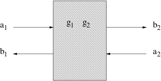
FIG. 1.: Quasi one-dimensional geometry of the device with definition of field input and output operators.

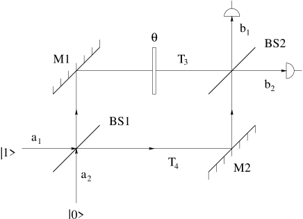
FIG. 2.: Mach–Zehnder interferometer with dispersive and absorbing beam splitters BS1 and BS2 and a phase shift $\Theta$. The mirrors M1 and M2 as well as the branches between BS1 and BS2 are assumed to be lossy with transmittance $T_{3}$ (upper branch) and $T_{4}$ (lower branch), respectively.

FIG. 3.: Entanglement created at a lossless beam splitter with both input modes excited in an one-photon Fock state. The entanglement is shown in exponential scaling vs. transmittance. Maximal entanglement $\ln 3$ is created at a $20\%/80\%$ beam splitter whereas for a symmetric device it drops to $\ln 2$ due to destructive interference.

FIG. 4.: The reflection coefficient $|R|^{2}$ (full line), the transmission coefficient $|T|^{2}$ (dashed line), and the absorption coefficient $(1$ $\!-$ $|R|^{2}$ $\!-$ $\!|T|^{2})$ (dotted line) of a dielectric plate are shown as functions of frequency $\omega$ for $\epsilon_{\rm s}$ $\!=$ $\!1.5$ and $\gamma/\omega_{0}$ $\!=$ $\!0.001$ in Eq. (25), and the plate thickness $2c/\omega_{0}$.

FIG. 5.: Frequency dependence of the entanglement measure $E(\hat{\sigma})$ (dashed line) and the total correlation $I_{c}$ (solid line) for a state $|1,0,0,0\rangle$ impinging on a beam splitter with $\gamma/\omega_{0}$ $\!=$ $\!0.001$ in Eq. (25) and the other parameters given in the text.

FIG. 6.: Frequency dependence of the entanglement measure $E(\hat{\sigma})$ (dashed line) and the total correlation $I_{c}$ (solid line) for a state $|1,1,0,0\rangle$ impinging on a beam splitter with $\gamma/\omega_{0}$ $\!=$ $\!0.001$ in Eq. (25) and the other parameters given in the text.

FIG. 7.: Frequency dependence of the entanglement measure $E(\hat{\sigma})$ (dashed line) and the total correlation $I_{c}$ (solid line) for a state $|1,0,0,0\rangle$ impinging on a beam splitter with $\gamma/\omega_{0}$ $\!=$ $\!0.01$ in Eq. (25) and the other parameters given in the text.

FIG. 8.: Entanglement degradation of a singlet state $|\Psi^{-}_{n}\rangle\langle\Psi^{-}_{n}|$ [Eq. (26)] with one photon ($n\!=\!1$ full curve) and two photons ($n\!=\!2$ dashed curve) after transmission through absorbing channels of equal transmittance.

FIG. 9.: Comparison of entanglement degradation of one-photon Bell basis states $|\Phi^{\pm}\rangle$ (full curve) and $|\Psi^{\pm}\rangle$ (dashed curve).

FIG. 10.: Entanglement degradation of a singlet state $|\Psi^{-}\rangle\langle\Psi^{-}|$ [Eq. (26) with $n$ $\!=$ $\!1$] after transmission of one subsystem (dashed curve) or both subsystems (full curve) through a medium with susceptibility (51).

REFERENCES

- [1] B. Huttner and S.M. Barnett, Phys. Rev. A 46, 4306, (1992).
- [2] J.J. Hopfield, Phys. Rev. 112, 1555 (1958).
- [3] T. Gruner and D.-G. Welsch, Phys. Rev. A 53, 1818 (1996).
- [4] Ho Trung Dung, L. Knöll, and D.-G. Welsch, Phys. Rev. A 57, 3931 (1998).
- [5] S. Scheel, L. Knöll, and D.-G. Welsch, Phys. Rev. A 58, 700 (1998).
- [6] R. Matloob, R. Loudon, S.M. Barnett, and J. Jeffers, Phys. Rev. A 52, 4823 (1995).
- [7] R. Matloob and R. Loudon, Phys. Rev. A 53, 4567 (1996).
- [8] T. Gruner and D.-G. Welsch, Phys. Rev. A 54, 1661 (1996).
- [9] S.M. Barnett, C. R. Gilson, B. Huttner, and N. Imoto, Phys. Rev. Lett. 77, 1739 (1996).
- [10] T. Gruner and D.-G. Welsch, Opt. Commun. 134, 447 (1997).
- [11] S.M. Barnett, J. Jeffers, A. Gatti, and R. Loudon, Phys. Rev. A 57, 2134 (1998).
- [12] J. Jeffers, S.M. Barnett, R. Loudon, R. Matloob, and M. Artoni, Opt. Commun. 131, 66 (1996).
- [13] J.R. Jeffers, N. Imoto, and R. Loudon, Phys. Rev. A 47, 3346 (1993).
- [14] M. Artoni and R. Loudon, Phys. Rev. A 57, 622 (1998).
- [15] M. Patra and C.W.J. Beenakker, Phys. Rev. A 61, 63805 (2000).
- [16] L. Knöll, S. Scheel, E. Schmidt, D.-G. Welsch, and A.V. Chizhov, Phys. Rev. A 59, 4716 (1999).
- [17] R.A. Campos, B.E.A. Saleh, and M.C. Teich, Phys. Rev. A 40, 1371 (1989).
- [18] U. Leonhardt, Phys. Rev. A 48, 3265 (1993).
- [19] V. Vedral and M.B. Plenio, Phys. Rev. A 57, 1619 (1998).
- [20] V. Vedral, M.B. Plenio, M.A. Rippin, and P.L. Knight, Phys. Rev. Lett. 78, 2275 (1997).
- [21] M. Horodecki, P. Horodecki, and R. Horodecki, Phys. Rev. Lett. 84, 2014 (2000).
- [22] M. Hendrych, M. Dušek, and O. Haderka, Proceedings of the 4th Central European Workshop on Quantum Optics (Budmerice, 1996) [Acta Phys. Slov. 46 393, 1996].
- [23] A. Wehrl, Rev. Mod. Phys. 50, 221 (1978).
- [24] M. Lewenstein and A. Sanpera, Phys. Rev. Lett. 80, 2261 (1998).
- [25] S.L. Braunstein and H.J. Kimble, Phys. Rev. Lett. 80, 869 (1998).
- [26] S.E. Harris and L.V. Hau, Phys. Rev. Lett. 82, 4611 (1999).
- [27] M.M. Kash, V.A. Sautenkov, A.S. Zibrov, L. Hollberg, G.R. Welch, M.D. Lukin, Y. Rostovstev, E.S. Fry, and M.O. Scully, Phys. Rev. Lett. 82, 5229 (1999).
- [28] M.D. Lukin, S.F. Yelin, and M. Fleischhauer, Phys. Rev. Lett. 84, 4232 (2000).
- [29] L.-M. Duan, G. Giedke, J.I. Cirac, and P. Zoller, Phys. Rev. Lett. 84, 2722 (2000); R. Simon, ibid. 84, 2726 (2000).
- [30] K.E. Cahill and R.J. Glauber, Phys. Rev. 177, 1857 (1969).
- [31] A.P. Prudnikov, Yu.A. Brychkov, and O.I. Marichev, Integrals and Series, Volume II: Special functions (Gordon and Breach, New York, 1986).
- [32] I.S. Gradshteyn and I.M. Ryzhik, Table of Integrals, Series, and Products (Academic Press, San Diego, 1994).