Local measurements of nonlocal observables and the relativistic reduction process

Abstract

In this paper we reconsider the constraints which are imposed by relativistic requirements to any model of dynamical reduction. We review the debate on the subject and we call attention on the fundamental contributions by Aharonov and Albert. Having done this we present a new formulation, which is much simpler and more apt for our analysis, of the proposal put forward by these authors to perform measurements of nonlocal observables by means of local interactions and detections. We take into account recently proposed relativistic models of dynamical reduction and we show that, in spite of some mathematical difficulties related to the appearence of divergences, they represent a perfectly appropriate conceptual framework which meets all necessary requirements for a relativistic account of wave packet reduction. Subtle questions like the appropriate way to deal with counterfactual reasoning in a relativistic and nonlocal context are also analyzed in detail.

1 Introduction

As it is well known, standard quantum mechanics is characterized by irreducible stochastic features which enter into play and give rise to puzzling situations in connection with the measurement process or, more appropriately and more generally, with the so called macro-objectification problem. It is useful to stress that it is precisely with reference to such processes which, when one takes further into account the unavoidable nonlocal character of the theory, the problem of the causal relations between events (such as the measurement outcome in one region and the transition from potential to actual physical situations in another) emerges as a central one. It goes without saying that an adequate discussion of such questions requires a relativistic approach. Our main concern here will be the analysis of statevector reduction in a relativistic quantum context and the identification of the basic features which any relativistic reduction mechanism must exhibit. In particular we will show that recent attempts in this direction [1]-[6], even though not fully satisfactory due to some technical problems (such as the appearence of untractable divergencies) have given clear indications about the line of thought one should follow to account for the nonlinear and stochastic reduction process meeting the strict demands of special relativity.

In section 2 we reconsider the crucial aspects of the problem under investigation by following the recent lucid presentation of the matter by Breuer and Petruccione [7]. Particular attention will be devoted to the fundamental contributions to the subject by Aharonov and Albert [8], [9] and [10]. These authors have identified the necessary formal features that any acceptable relativistic reduction mechanism must exhibit and have shown that all previous attempts in this direction were fundamentally unsatisfactory. The key argument which has led Aharonov and Albert to draw such a conclusion is their proof [9] that one can measure nonlocal observables by resorting to local interactions between appropriately (and smartly) chosen quantum systems, followed by local detection processes.

There are, however, two reasons which require to deepen and to improve the line of thought of these authors. First, their explicit example of a local measurement of nonlocal observables is quite formal and rests on the consideration of nonnormalizable states. Secondly, in spite of the fact that they have given clear indications about the general formal features of any acceptable relativistic dynamical reduction mechanism, they have made no attempt to work out an explicit example of such a dynamics. On the other hand, as already mentioned, in recent years precise relativistic models of dynamical reduction have been formulated [1]-[6]. It is one of the aims of this paper to investiagte critically such models from the point of view of the analysis of Aharonov and Albert.

To this purpose it is useful to work out, first of all, a remarkably simplified version of the measurement procedure suggested by the above authors in ref.[9]. This is achieved in section 3 by relating the relevant physical process to degrees of freedom whose associated Hilbert space is finite–dimensional. In this way the treatment turns out to be extremely simple and intuitive and the procedure easy to implement in practice. This simplified version of the proposal of ref.[9] will allow us to focus the essential features of any relativistic reduction theory and to show that such features are essential and natural ingredients of the theoretical framework presented in refs.[1]-[6]. Accordingly, in the rest of the paper we will discuss how such precise theoretical schemes account for the relativistic macro-objectification process and we will show that they lead to a perfectly coherent view which allows one to analyze basic issues such as the attribution of objective properties to individual physical systems, the necessary generalization of the concept of event and the appropriate way to resort to counterfactual arguments within a relativistic and nonlocal context.

2 Relativistic reduction processes

This section is devoted to reviewing some of the issues of the central theme of the paper, i.e., the relativistic aspects of the reduction process.

2.1 Local relativistic reduction processes

The main problems which one meets in trying to generalize the nonrelativistic process of statevector reduction derive from the assumed instantaneity of such a process. As lucidly described in ref.[7] one can consider the case in which one has a system whose associated wavefunction has an appreciable spatial extension and, at time $t=0,$ is found at $x=0$ by a detector which is placed there. The problem one has to face is quite obvious: even if one were able to account for the local position measurement in terms of a local covariant interaction between the measured object and the measuring device, the ensuing picture would obviously turn out not to be covariant for the very simple reason that in any other reference frame the space-like surface $t=0$ is not an equal time surface; consequently, the reduction cannot be instantaneous for any observer in motion with respect to the original one.

Hellwig and Kraus [11] have proposed to circumvent the above difficulty by postulating that in a local measurement process statevector reduction takes place along the past light cone originating from the space-time point at which the covariant system-apparatus interaction occurs. In contrast with the case mentioned above it is obvious that the proposed prescription is manifestly covariant since the light cone from a given point is the same in all reference frames. These authors have also shown that their prescription leads to the correct quantum predictions concerning the probabilities of the outcomes of local measurements of local observables. In the early stages of the debate about relativistic reduction processes the expression “local” has been used in a quite loose way which we will follow in this subsection with the purpose of making quite intuitive the problems one meets. Suppose our system, let us say an elementary particle, prior to the local position measurement at $t=0,$ $x=0,$ is described, in a given reference frame, by a wavefunction which has an appreciable extension in space (the limiting case would be the one of a system in a state of definite momentum). A measurement in which the particle is found at $x=0$ will, according to the Hellwig and Kraus prescription, lead to a statevector which is different from zero only within the past light cone from the origin, contradicting the fact that at a time prior to $t=0$ the wavefunction extends over a much larger region as, e.g., in the limiting case of a momentum eigenstate, which, if subjected to a momentum measurement, would remain unaltered. According to Hellwig and Kraus the way out from such a difficulty derives from assuming that, e.g., the alleged momentum measurement cannot be performed by resorting to local interactions. Actually, already in 1931, Landau and Peierls [12] had suggested that all nonlocal quantities, like the momentum operators, cannot be considered as observables in relativistic quantum theories. Hellwig and Kraus adopt this point of wiev and, consequently, they dismiss as non pertinent any criticism concerning their proposal. Here comes the fundamental contribution by Aharonov and Albert [9]. They have shown that it is actually possible to measure nonlocal observables and, even more important, that this can be done by local interactions and local detections.

Before going on, it is appropriate to stress a point of great conceptual relevance for the subject of this paper. In the debate we have just reviewed it was always assumed (more or less tacitly) that the wavefunction $\Psi(x,t),$ in the relativistic case must be considered as a function on the space-time continuum. As we will see, the analysis of Aharonov and Albert requires a radical change of perspective about this fact.

2.2 Nonlocal measurements in a relativistic context and their difficulties

As already anticipated, within a relativistic context, nonlocal observables raise particular problems in connection with measurement processes. To better focus this point, in place of the rather vague considerations of the previous subsection related to momentum measurements, we present a slightly modified version of a simple and nice example by Breuer and Petruccione [7].

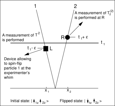
Figure 1: An ideal experiment which points out the restrictions on nonlocal measurements imposed by causality

Let us consider (Fig.1) a given inertial reference frame and a pair of particles having space plus internal degrees of freedom. For simplicity, since these assuptions do not change in any way whatsoever the conceptually relevant aspects of the analysis, we will disregard the spreading of the wavepackets of the two particles and we will assume that the internal degrees of freedom refer to quantities, like the isospin, which do not transform under Lorentz transformations. Suppose the two particles are created, e.g., in a decay process at a given objective space-time point and that they propagate in opposite directions. Concerning the internal degrees of freedom, let us assume that the two particles have isospin $1/2$ and are in the common eigenstate of $T^{2}$ and $T_{z}$ belonging to the eigenvalues (in the appropriate units) $2$ and $1$, respectively, i.e., in the state we will denote (in analogy with the case of spin variables) as $|\uparrow_{1z},\uparrow_{2z}>.$ Suppose that, along the world line of particle 1 (the one propagating at left), at a precise space-time point $L(x_{1},t_{1}-\epsilon)$, there is a device which can be switched on and off at the experimenter’s whim, whose only (local) effect is that of inducing a isospin flip of the particle interacting with it when it is on, while no change occurs when it is off. Suppose also that, at time $t_{1}$, a measurement of the nonlocal observable $T^{2}$ is performed on the composite system. We stress that since the two particles are in different space regions the measurement of $T^{2}$ is unavoidably nonlocal. Finally let us assume that at time $t_{1}+\epsilon,$ at a point $R(x_{2},t_{1}+\epsilon)$ on the world line of particle 2 there is an apparatus measuring $T_{2z},$ the $z$ component of the isospin of particle 2.

Given these premises one can argue as follows:

• Suppose the apparatus at $L$ is off. Then the state of the composite system at $t_{1}$ is $|\uparrow_{1z},\uparrow_{2z}>,$ which, being an eigenstate of $T^{2},$ is left unchanged by the measurement of this observable. There follows that in the subsequent measurement of $T_{2z}$ the outcome +1 is obtained with certainity.

• Suppose now the apparatus at $L$ is on. Then the state of the composite system at $t_{1}-\epsilon$ becomes $|\downarrow_{1z},\uparrow_{2z}>,$ which is the superposition with equal squared amplitudes of the eigenstates of $T^{2}$ belonging to the eigenvalues 0 and 2, respectively. The measurement taking place at $t_{1}$ will then reduce the state to one of such eigenstates, i.e., $\frac{1}{\sqrt{2}}[|\downarrow_{1z},\uparrow_{2z}>\mp$ $|\uparrow_{1z},\downarrow_{2z}>],$ which assign probability $1/2$ both to the outcome +1 and to –1 in the measurement of $T_{2z}$ at $t_{1}+\epsilon$. If the observer at $R$ is informed about the experimental set-up, in the cases in which he gets the outcome –1 he can infer that the observer at $L$ has actually decided to induce the spin flip of particle 1. This argument shows quite nicely that nonlocal measurements can lead to a violation of causality allowing superluminal communication and makes clear while such measurements must be excluded if one wants to take the position of Hellwig and Kraus about statevector reduction.

2.3 The Aharonov and Albert procedure

The simplest example of a measurement of a nonlocal observable proposed by these authors is, in our language, a measurement of the $z-$component of the total isospin $T_{z}=T_{1z}+T_{2z}$ of the previous system. The smart trick consists in considering an apparatus constituted by two subsystems (probes) whose world lines intersect the world lines of particles 1 and 2 (once more we disregard the spreading associated with the free motion of the probes) and considering “internal generalized coordinates $\widehat{q}_{1}$ and $\widehat{q}_{2}$”of the probes. The local interactions of the probes with the particles are described by the hamiltonian:

$$H_{I}=g(t)\left[\widehat{q}_{1}T_{1z}+\widehat{q}_{2}T_{2z}\right],$$ (2.1)

where $g(t)$ is a time dependent coupling constant vanishing outside a small time interval $(t_{1},t_{2})$. Finally, one assumes that the probes are, at any time $t_{0}$ preceeding their interactions with the particles, in an entangled state of the kind of the one considered in the celebrated EPR paper, i.e., one in which both the coordinates $\widehat{q}_{1}$ and $\widehat{q}_{2}$ and the conjugated momenta $\widehat{\pi}_{1}$ and $\widehat{\pi}_{2}$ are perfectly correlated:

$$\widehat{\pi}_{1}(t_{0})+\widehat{\pi}_{2}(t_{0})=0$$

$$\widehat{q}_{1}(t_{0})-\widehat{q}_{2}(t_{0})=0.$$ (2.2)

As in the standard measurement scheme by von Neumann the local interactions described by eq.(2.1) imply the following equation of motion for the total canonical momentum $\pi(t)$:

$$\frac{\partial\pi(t)}{\partial t}=i[H_{I},\pi(t)]=-g(t)\left[T_{z1}+T_{z2}\right]=-g(t)T_{z,}$$ (2.3)

so that one can infer the value of $T_{z}$ from the change of the total momentum:

$$T_{z}=-\frac{\pi(t>t_{2})}{\int_{t_{1}}^{t_{2}}dtg(t)},$$ (2.4)

where we have taken into account that $\pi(t<t_{1})=0,$ as shown by the first of eqs.(2.2). To make eq.(2.4) more understandable to the reader, we remark that the local interaction of one probe with the corresponding particle decreases (increases) the value of the associated momentum according whether the particle is in the eigenstate $T_{iz}=+1$ $(-1),$ respectively. Accordingly, the total momentum changes when the two particles have parallel $z-$isospin components and remains unchanged when their projections are opposite.

It is extremely important to realize that the measurement is a genuinely nonlocal measurement performed by means of local interactions and detections. In fact it is easy to convince oneselves that the knowledge, after the measurement, of the value of the momentum of only one of the probes does not allow to draw any conclusion referring to the isospin component of the particle which has interacted with the probe, or to the component of the total isospin. This point will become much more clear when we will consider the simplified version of a measurement of this kind which is the subject of the following Section.

Some remarks are at order:

• The two probes considered in refs.[9] have translational degrees of freedom related to their propagation and interactions with the particles and further internal degrees of freedom which, however, are associated to continuous generalized coordinates and momenta. Moreover, the state of the probes before the measurement exhibits perfect “internal” momentum and position correlations, just as the state of the original EPR argument. Leaving aside the problem of the difficulty of preparing such an entangled state in these continuous variables, the resulting state turns out to be nonnormalizable. It should be clear to the reader that the very cute proposal by Aharonov and Albert corresponds to a quite idealized situation. Just in the same way in which Bohm has felt the necessity of rephrasing the EPR argument resorting to the consideration of spin degrees of freedom, transforming it from a gedanken to a feasible experiment, we consider it useful to perform an analogous step with reference to the process under discussion.

• The above procedure has been generalized by the authors of refs.[9] to measure the square $T^{2}$ of the total isospin of the composite system. Such a step involves the use of three pairs of entangled probes which interact with particles 1 and 2. Only the comparison of the outcomes obtained at the two wings of the apparatuses devised to measure the momenta of the three probes allows, in the case in which all pairs of momenta sum up to zero, to assert that the system has been found in the singlet state. The measurement is fundamentally a quantum nondemolition measurement for the singlet state, while it is not a measurement of the standard type for the states of the three dimensional manifold $T^{2}=2.$ Once more these subtle questions will become clear in the modified version of a local measurementof nonlocal observables we are going to discuss.

3 A new procedure for a local measurement of nonlocal observables

In this Section we present a possible experimental setup for the measurement of the observables $T_{z}$ and $T^{2}$ of the system S of two particles of isospin 1/2 which is based on local interactions between the particles and probe particles whose internal degrees of freedom are accounted by the states of a three-dimensional Hilbert space (Fig.2).

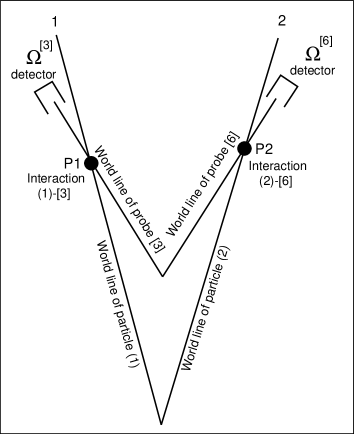
Figure 2: The way to perform a nonlocal measurement by resorting to local interactions and detections.

To begin, we consider, as before, two particles 1 and 2 which are produced at a given space-time point and propagate along two world lines. Since we disregard the spreading of the wavefunctions of the particles, their quantum features are entirely described by the vectors of the four-dimensional Hilbert spaced spanned by the states (with obvious meaning of the symbols):

$$|\uparrow_{1z},\uparrow_{2z}>,\qquad|\uparrow_{1z},\downarrow_{2z}>,\qquad|\downarrow_{1z},\uparrow_{2z}>,\qquad|\downarrow_{1z},\downarrow_{2z}>.$$ (3.1)

We consider also a system $\Sigma$ of two probe particles (which for reasons which will become clear in what follows we identify as 3 and 6) whose world lines intersect, at the space time points $P1$ and $P2$, the world lines of the system particles. The probe particles, as already stated, besides their configurational degrees of freedom (which we treat once more as classical), have internal degrees of freedom associated to a three-dimensional Hilbert space. We denote as

$$|-1>_{i},\qquad|0>_{i},\qquad|+1>_{i},\qquad(i=3,6),$$ (3.2)

the complete set of the eigenstates of an observable $\Omega^{(i)}$ of the Hilbert space of the i-th probe and by

$$|a,b>_{3,6}\equiv|a>_{3}\otimes|b>_{6},\qquad(a,b=-1,0,+1)$$ (3.3)

the elements of the corresponding basis in the nine-dimensional Hilbert space of $\Sigma$. The initial state of the probe is assumed to be the normalized entangled state of particles 3 and 6:

$$|\Phi>_{3,6}=\frac{1}{\sqrt{3}}\left[|0,0>_{3,6}+|+1,-1>_{3,6}+|-1,+1>_{3,6}\right].$$ (3.4)

The system and probe particles interact locally (constituent 1 (2) of $S$ with constituent 3 (6) of $\Sigma$) for a given time interval, the effect of the interaction being described by the unitary operator $U_{z}:$

$$U_{z}=\left[P_{z+}^{(1)}P_{L}^{(3)}+P_{z-}^{(1)}P_{R}^{(3)}\right]\otimes\left[P_{z+}^{(2)}P_{L}^{(6)}+P_{z-}^{(2)}P_{R}^{(6)}\right],$$ (3.5)

where the operators $P^{(i)}_{z\pm}$ are the projection operators on the eigenmanifolds of $T_{iz}$:

$$P_{z+}^{(i)}=|\uparrow_{iz}><\uparrow_{iz}|,\qquad P_{z-}^{(i)}=|\downarrow_{iz}><\downarrow_{iz}|,\qquad(i=1,2)$$

and the operators $P^{(j)}_{R,L}$ act on the probe space and have, in the basis (3.2), the representation indicated below:

$$P_{L}^{(j)}=\left(\begin{array}[]{lll}0&0&1\\ 1&0&0\\ 0&1&0\end{array}\right)_{j},\qquad P_{R}^{(j)}=\left(\begin{array}[]{lll}0&1&0\\ 0&0&1\\ 1&0&0\end{array}\right)_{j},\qquad(j=3,6).$$ (3.6)

We note that the operators $P_{L}^{(j)}$ and $P_{R}^{(j)}$ act in the following way on the states of the base of probe j:

$$P_{L}^{(j)}|-1>_{j}=|+1>_{j},\qquad P_{L}^{(j)}|0>_{j}=|-1>_{j},\qquad P_{L}^{(j)}|+1>_{j}=|0>_{j},$$ (3.7)

$$P_{R}^{(j)}|-1>_{j}=|0>_{j},\qquad P_{R}^{(j)}|0>_{j}=|+1>_{j}\qquad P_{R}^{(j)}|+1>_{j}=|-1>_{j},$$ (3.8)

so that they produce an anticlockwise and a clockwise permutation of the three states ($|-1>,|0>,|+1>$) of the basis, respectively. We also note the following properties of these operators:

$$P_{R}^{(j)\dagger}=P_{L}^{(j)},\qquad P_{L}^{(j)\dagger}=P_{R}^{(j)},\qquad P_{R}^{(j)}P_{L}^{(j)}=P_{L}^{(j)}P_{R}^{(j)}=1^{(j)}.$$ (3.9)

The above relations imply:

$$U_{z}^{\dagger}U_{z} = \left[P_{z+}^{(1)}P_{R}^{(3)}+P_{z-}^{(1)}P_{L}^{(3)}\right]\otimes\left[P_{z+}^{(2)}P_{R}^{(6)}+P_{z-}^{(2)}P_{L}^{(6)}\right]\cdot$$

$$\left[P_{z+}^{(1)}P_{L}^{(3)}+P_{z-}^{(1)}P_{R}^{(3)}\right]\otimes\left[P_{z+}^{(2)}P_{L}^{(6)}+P_{z-}^{(2)}P_{R}^{(6)}\right]$$

$$= \left[P_{z+}^{(1)}1^{(3)}+P_{z-}^{(1)}1^{(3)}\right]\left[P_{z+}^{(2)}1^{(6)}+P_{z-}^{(2)}1^{(6)}\right]=1^{(1)}1^{(2)}1^{(3)}1^{(6)}=1,$$

so that $U_{z}$ is a unitary operator.

Given the above equations it is immediate to evaluate the effect of applying $U_{z}$ to the direct product of any one of the states (3.1) times the initial state of the probe $|\Phi>_{3,6}.$ To this purpose it is useful to introduce the following normalized states of the probe system (with obvious meaning of the symbols):

$$|\Pi(1,-2)>_{3,6} = \frac{1}{\sqrt{3}}\left[|-1,-1>_{3,6}+|0,+1>_{3,6}+|+1,0>_{3,6}\right]$$ (3.11)

$$|\Pi(2,-1)>_{3,6} = \frac{1}{\sqrt{3}}\left[|+1,+1>_{3,6}+|0,-1>_{3,6}+|-1,0>_{3,6}\right].$$

As easily checked we then have:

$$U_{z}\left[|\uparrow_{1z},\uparrow_{2z}>\otimes|\Phi>_{3,6}\right] = |\uparrow_{1z},\uparrow_{2z}>\otimes|\Pi(1,-2)>_{3,6}$$ (3.12)

$$U_{z}\left[|\downarrow_{1z},\downarrow_{2z}>\otimes|\Phi>_{3,6}\right] = |\downarrow_{1z},\downarrow_{2z}>\otimes|\Pi(2,-1)>_{3,6}$$

$$U_{z}\left[|\uparrow_{1z},\downarrow_{2z}>\otimes|\Phi>_{3,6}\right] = |\uparrow_{1z},\downarrow_{2z}>\otimes|\Phi>_{3,6}$$

$$U_{z}\left[|\downarrow_{1z},\uparrow_{2z}>\otimes|\Phi>_{3,6}\right] = |\downarrow_{1z},\uparrow_{2z}>\otimes|\Phi>_{3,6}$$

The model we have presented, in complete analogy with the one proposed by Aharonov and Albert, describes a nonlocal measurement procedure (in terms of local interactions and detections) of the nonlocal observable $T_{z},$ the z-component of the total isospin of the composite system $S$. In fact, in order to complete the measurement, we have only to put on the world lines of the probe particles two apparata measuring the observables $\Omega^{(i)}$(i=3,6), to register the obtained outcomes and to sum them. If they sum up to 0, then reduction takes place to a state for which $T_{z}=0,$ if they sum up to either 1 or –2 then reduction takes place to the state for which $T_{z}=1,$ finally, if they sum up to either 2 or –1, reduction takes place to the state for which $T_{z}=-1.$

It is of great relevance to remark that for each of the states of the probes appearing at the right hand side of eq.(3.12) all possible eigenvalues ($\omega_{k}^{(i)}=-1,0,1)$ of the observable $\Omega^{(i)}$ referring to each probe particle appear with equal weights. Thus, knowledge of the outcome, e.g., of the detector at the right wing of the apparatus, does not give any information whatsoever about the isospin component of the particle with which the probe particle has interacted locally, nor about the component of the total isospin. In this precise sense the measurement is genuinely nonlocal (as it must be, since the two particles lie in far apart regions).

We can now proceed to generalize the previous procedure to a measurement process for $T^{2}.$ To this purpose we have to resort to a more complicated device corresponding to the production of three entangled pairs of probe particles which interact locally with the particles whose total isospin is being measured. So, besides the pair (3-6) of probe particles we will consider also the pairs (2*-4*) and (3*-6*). The initial state of the whole probe will simply be the direct product of three states like (3.4):

$$|\Phi>=|\Phi>_{3*,6*}\otimes|\Phi>_{2*,4*}\otimes|\Phi>_{3,6}$$ (3.13)

and the unitary evolution operator $U$ for the whole system is assumed to be the product of three operators: $\widetilde{U}_{z}U_{y}U_{z}$. In turn, $U_{z}$ is the operator defined in (3.5), $U_{y}$ has exactly the same form of $U_{z}$ with the operators $P_{y+}^{(1)},P_{y-}^{(1)},P_{y+}^{(2)},P_{y-}^{(2)}$ replacing the corresponding ones with the index $z$, and the operators $P_{L}^{(2*)},P_{R}^{(2*)},P_{L}^{(4*)},P_{R}^{(4*)}$ replacing the corresponding ones with the indices $3$ and $6$. Finally $\widetilde{U}_{z}$ coincides with $U_{z}$ with the replacement of the indices 3 and 6 by the corresponding indices 3* and 6*.

To see how the mechanism works we have, first of all, to express the states (3.1) in terms of the corresponding states of the type $|\uparrow_{1y},\uparrow_{2y}>$ etc., in order to evaluate the effetct of applying the operator $U_{y}.$ Moreover, since now we are interested in identifying the eigenstates of $T^{2}$, it is useful to replace the states $|\uparrow_{1z,}\downarrow_{2z}>$ and $|\downarrow_{1z,}\uparrow_{2z}>$ by their simmetrical and skew-symmetrical combinations:

$$|Triplet>_{z} = \frac{1}{\sqrt{2}}\left[|\uparrow_{1z},\downarrow_{2z}>+|\downarrow_{1z},\uparrow_{2z}>\right],$$ (3.14)

$$|Singlet>_{z} = \frac{1}{\sqrt{2}}\left[|\uparrow_{1z},\downarrow_{2z}>-|\downarrow_{1z},\uparrow_{2z}>\right]$$

and analogous ones for the states $|\uparrow_{1y,}\downarrow_{2y}>$ and $|\downarrow_{1y,}\uparrow_{2y}>$.

With these premises an elementary (but tedious) calculation shows the effect of applying the unitary operator $U$ to the isospin singlet and triplet states:

$$U|Singlet>\otimes|\Phi>=|Singlet>\otimes|\Phi>$$ (3.15)

$$U|\uparrow_{1z},\uparrow_{2z}>\otimes|\Phi>=$$

$$+\left\{\frac{1}{4}|\Pi(1,-2)>_{3*,6*}\otimes\left[|\Pi(1,-2)>_{2*,4*}+|\Pi(2,-1)>_{2*,4*}+2|\Phi>_{2*,4*}\right]\otimes|\uparrow_{1z},\uparrow_{2z}>\right.$$

$$-\frac{1}{4}|\Pi(2,-1)>_{3*,6*}\otimes\left[|\Pi(1,-2)>_{2*,4*}+|\Pi(2,-1)>_{2*,4*}-2|\Phi>_{2*,4*}\right]\otimes|\downarrow_{1z},\downarrow_{2z}>$$

$$\left.+\frac{i}{2\sqrt{2}}|\Phi>_{3*,6*}\otimes\left[|\Pi(1,-2)>_{2*,4*}-|\Pi(2,-1)>_{2*,4*}\right]|Triplet>_{z}\right\}\otimes|\Pi(1,-2)>_{3,6};$$

$$U|\downarrow_{1z},\downarrow_{2z}>\otimes|\Phi>=$$

$$\left\{-\frac{1}{4}|\Pi(1,-2)>_{3*,6*}\otimes\left[|\Pi(1,-2)>_{2*,4*}+|\Pi(2,-1)>_{2*,4*}-2|\Phi>_{2*,4*}\right]\otimes|\uparrow_{1z},\uparrow_{2z}>\right.$$

$$+\frac{1}{4}|\Pi(2,-1)>_{3*,6*}\otimes\left[|\Pi(1,-2)>_{2*,4*}+|\Pi(2,-1)>_{2*,4*}+2|\Phi>_{2*,4*}\right]\otimes|\downarrow_{1z},\downarrow_{2z}>$$

$$\left.-\frac{i}{2\sqrt{2}}|\Phi>_{3*,6*}\otimes\left[|\Pi(1,-2)>_{2*,4*}-|\Pi(2,-1)>_{2*,4*}\right]|Triplet>_{z}\right\}\otimes|\Pi(2,-1)>_{3,6};$$

$$U|Triplet>_{z}\otimes|\Phi>=$$

$$\left\{-\frac{i}{2\sqrt{2}}|\Pi(1,-2)>_{3*,6*}\otimes\left[|\Pi(1,-2)>_{2*,4*}-|\Pi(2,-1)>_{2*,4*}\right]\otimes|\uparrow_{1z},\uparrow_{2z}>\right.$$

$$+\frac{i}{2\sqrt{2}}|\Pi(2,-1)>_{3*,6*}\otimes\left[|\Pi(1,-2)>_{2*,4*}-|\Pi(2,-1)>_{2*,4*}\right]\otimes|\downarrow_{1z},\downarrow_{2z}>$$

$$\left.+\frac{1}{2}|\Phi>_{3*,6*}\otimes\left[|\Pi(1,-2)>_{2*,4*}+|\Pi(2,-1)>_{2*,4*}\right]\otimes|Triplet>_{z}\right\}\otimes|\Phi>_{3,6}.$$

Suppose now that there are six local detectors (three at each wing) devised to measure the observables $\Omega^{(s)},$ $s=$ 3,6,2*,4*,3*,6* and denote as $\omega^{(s)}$ the obtained outcomes. The above relations exhibit some interesting features:

i). If $\omega^{(3)}+\omega^{(6)}=\omega^{(2*)}+\omega^{(4*)}=\omega^{(3*)}+\omega^{(6*)}=0,$ then reduction has taken place to $|Singlet>.$

ii). If at least one of the relations under i) is not satisfied, reduction has taken place to a state belonging to the three-dimensional $T^{2}=2$ eigenmanifold.

This second case can be further analyzed according to the following table:

$$\begin{array}[]{clclcl}\makebox{If}&\omega^{(3*)}+\omega^{(6*)}&=&\makebox{$1$ or $-2$}&\makebox{reduction has taken place to}&|\uparrow_{1z},\uparrow_{1z}>\\ \makebox{If}&\omega^{(3*)}+\omega^{(6*)}&=&\makebox{$2$ or $-1$}&\makebox{reduction has taken place to}&|\downarrow_{1z},\downarrow_{1z}>\\ \makebox{If}&\omega^{(3*)}+\omega^{(6*)}&=&\makebox{$0$ and $\omega^{(2*)}+\omega^{(4*)}\neq 0$}&\makebox{reduction has taken place to}&|Triplet>_{z}.\end{array}$$

We can consider now an arbitrary state of the system, i.e. a linear superposition of the four states (3.1),

$$|\Psi>=\alpha|\uparrow_{1z},\uparrow_{2z}>+\beta|\uparrow_{1z},\downarrow_{2z}>+\gamma|\downarrow_{1z},\uparrow_{2z}>+\delta|\downarrow_{1z},\downarrow_{2z}>$$ (3.19)

and use it to trigger our measuring devices. The resulting state $U|\Psi>\otimes|\Phi>$ will be the linear combination with the same coefficients of the states at the right hand side of eqs.(3.15-3.18). Let us write, for simplicity such a state as:

$$U|\Psi>\otimes|\Phi>=\eta|Singlet>\otimes|\Phi>+|\Gamma>.$$ (3.20)

As already remarked, if the detection procedure of the probe particles indicates that $\omega^{(3)}+\omega^{(6)}=\omega^{(2*)}+\omega^{(4*)}=\omega^{(3*)}+\omega^{(6*)}=0$ (and this occurs with probability $|\eta|^{2}$) then reduction takes place to the state $|Singlet>.$ In all other cases, even though reduction leads to a state of the eigemanifold $T^{2}=2,$ the measurement process does not respect the request of being “moral”, i.e., the condition that the reduced state be the (normalized) projection of the state prior to the measurement on the considered eigenmanifold. Said differently, the measurement, when it yields the outcome $T^{2}=2,$ turns out to be distorting for $T_{z}$. This is immediately seen by choosing in (3.19) $\beta=\gamma=\delta=0$ and by looking at eq.(3.16) which shows that there is a nonzero probability that the measurement leads to reduction on one of the states $|\downarrow_{z1},\downarrow_{z2}>$ and $|Triplet>_{z}.$ This is naturally related to the fact that, in a loose sense, one could state that in order to measure $T^{2}$ one has to measure simultaneously incompatible observables, such as $T_{1z}$ and $T_{1x,}$ of one of the particles. But for our purposes this nonideality of the measurement for the states of the eigenmanifold $T^{2}=2,$ is not relevant.

Actually, the feature of the measurement process we have just analyzed, besides being unavoidable, is an extremely positive one. In fact, if consideration is given to the situation discussed in Subsection 2.2, one easily sees that the distorting nature of the measurement eliminates the possibility of faster than light effects. From eq.(3.16) one sees that if a measurement of $T^{2}$ is performed on the state $|\uparrow_{1z},\uparrow_{2z}>$, the probability of getting in a subsequent measurement the outcome $T_{2z}=+1$ is no more equal to 1, but precisely to $1/2$. This agrees with the probability of getting such an outcome if one performs the measurement of $T^{2}$ on the state which has been subjected to a spin flip of particle 1, i.e. the state $|\downarrow_{1z},\uparrow_{2z}>$, as one derives immediately from a combined use of eqs.(3.15) and (3.18). On the contrary, eqs.(3.12) show that a local measurement of the nonlocal observable $T_{z}$ does not alter the fact that the probability of getting the outcome $T_{2z}=+1$ remains unaltered (and equal to 1) when the spin of particle 1 is flipped.

It is time to come to discuss the conceptual implications of the actual possibility of measuring nonlocal observables identified by Aharonov and Albert and reformulated by us in this Section.

4 The implications of the request of a covariant reduction

The analysis of ref.[9] and of the previous section rules out the Hellwig and Kraus proposal for a covariant reduction mechanism and requires to consider an alternative approach to the problem. This has been suggested in another important paper [10] by Aharonov and Albert. The proposal is quite simple and natural, but it has far reaching consequences. One could describe it by stating that, in a certain sense, they assume that reduction takes place instantaneously in all inertial frames. To be more clear, let us consider an objective space-time point $P$ where a local measurement occurs and the set of all space-like hyperplanes through $P.$ Each such hyperplane is a $t=const$ surface for an appropriate observer. The proposal of ref.[10] can then be formulated by stating that, for the considered reference frame, reduction takes place precisely along the $t=const$ hyperplane through $P.$

Note that this rule is manifestly covariant and it is quite natural, since the scope of statevector reduction is to allow one to exploit the information gained in a measurement for evaluating the probabilities of future (for him) events. However, taking such a position has far reaching consequences and requires a radical revision of the meaning of the wavefunction. Namely, the wavefunction cannot any longer be seen as a function on the space-time continuum but it becomes a function on the set of space-like hypersurfaces: the value of $\Psi$ at a space-time point depends, in general, on the particular space-time surface crossing the point we take into account. We should then write, in place of $\Psi(x,t),$ $\Psi=\Psi(\sigma,x),$ where $x$ runs over the points of the hypersurface $\sigma.$

An intuitive understanding of this fact can be obtained by considering (Fig.3) an objective space-time point $P$ at which a local position measurement occurs for a particle in a state which is different from zero along two distinct world lines ($l_{1}$ and $l_{2})$.

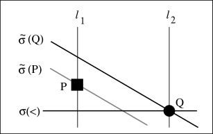
Figure 3: Illustration of the fact that in a relativistic context with reductions the statevector cannot be considered as a function on space time when local measurements are taken into account.

For a given reference frame, we can consider the set of $t=const$ hyperplanes. Then, for one of such hyperplanes $\sigma(<)$ associated to a time prior to the one characterizing the hyperplane through $P$, the wavefunction has a value different from zero at the point $Q$ in which $\sigma(<)$ intersects $l_{2}:$ $\Psi({\sigma}(<),Q)\neq{0}.$ We can now consider another reference frame such that in it, the $t=const$ hyperplane $\widetilde{\sigma}(Q)$ through $Q$ is characterized by a time label greater than the one characterizing the hyperplane $\widetilde{\sigma}(P)$ of the same family going through $P.$ If we suppose that in the local measurement the particle is detected at $P$ (note that this is an objective, i.e., reference frame independent statement), then we have: $\Psi(\widetilde{\sigma}(Q),Q)=0.$ Thus, according to the Aharonov and Albert proposal, the wavefunction must take different values at the same space-time point according to which space-like surface passing through it we take into account.

We conclude this section by remarking that the idea that to deal with relativistic quantum systems one must associate different statevectors to different space-like hypersurfaces is a quite hold one, going back to the fundamental papers by Tomonaga and Schwinger [13]. However, within the formalism proposed by these authors, the expectation value of any local observable having its compact support contained in the common part of two hypersurfaces (and thus in particular the value of the wavefunction at a point in which two such surfaces intersect) does not depend on which of the surfaces one is taking into account. This is not surprising: the Tomonaga-Schwinger theory is intended to describe (within a relativistic context) the linear and deterministic evolution of statevectors and does not pretend to account for nonlinear and stochastic processes like those we are considering here, i.e., the reduction processes.

5 Relativistic dynamical reduction theories

As repeatedly stressed in the previous sections, Aharonov and Albert, in their fundamental papers, have identified the crucial problems of relativistic reduction processes and have given clear hints about the features of any theory which should account for their occurrence. But they have not proposed any explicit and consistent dynamical mechanism specifying what occurs during a measurement process. Identifying such a new (universal) mechanism is precisely the aim of dynamical reduction theories.

5.1 The GRW theory

The first consistent and precise proposal of a dynamical theory accounting, at the nonrelativistic level, for the nonlinear and stochastic reduction process is the so called GRW theory [14]. As pointed out by Bell [15], this approach corresponds to accepting that Schrödinger’s equation is not always right and taking into consideration stochastic and nonlinear modifications of it which allow a unified treatment of all natural processes including the objectification of macroscopic properties. The model is based on the assumption that besides the standard quantum evolution, physical systems are subjected to spontaneous localizations occurring at random times with an appropriate average frequency and affecting their elementary constituents. Such processes are formally described in the following way.

Let us consider a system of $N$ particles. When the $i$-th particle of the system suffers a localization, the wavefunction changes according to

$$\Psi({\mathbf{r}}_{1},...,{\mathbf{r}}_{N})\Rightarrow\Psi_{\mathbf{x}}({\mathbf{r}}_{1},...,{\mathbf{r}}_{N})=\frac{\Phi_{\mathbf{x}}({\mathbf{r}}_{1},...,{\mathbf{r}}_{N})}{\left\|\Phi_{\mathbf{x}}\right\|}$$ (5.1)

$$\Phi_{\mathbf{x}}({\mathbf{r}}_{1},...,{\mathbf{r}}_{N})=\left(\frac{\alpha}{\pi}\right)^{\frac{3}{4}}e^{-\frac{\alpha}{2}({\mathbf{r}}_{i}-{\mathbf{x}})^{2}}\Psi({\mathbf{r}}_{1},...,{\mathbf{r}}_{N}).$$ (5.2)

The probability density of the process occurring at point x is given by $\left\|\Phi_{\mathbf{x}}\right\|^{2}.$ For what concerns the temporal aspects of the process we assume that the localizations of the various constituents (particles) occur independently at randomly distributed times with a mean frequency $\lambda_{m}$ which depends on their mass. We choose $\lambda_{m}=\lambda(m/m_{0})$, where $m$ is the mass of the particle, $m_{0}$ the nucleon mass and $\lambda$ is of the order of $10^{-16}\sec^{-1}.$ The localization parameter $1/{\sqrt{\alpha}}$ is assumed to take the value $10^{-5}cm$.

As the reader can easily grasp the model does not entail any appreciable deviation from standard quantum mechanics for microsystems since such systems suffer, on the average, one localization every $10^{9}$ years. The most appealing feature of the model derives from its trigger (or amplification) mechanism: in the case of a macroscopic system the frequency of the localizations is amplified with the number of its constituents and, in the case of an almost rigid body, each localization process amounts to a localization of the centre of mass, so that superpositions corresponding to different locations of a macroscopic object are suppressed in about $10^{-7}\sec$.

The physically relevant features of the just described model for what concerns the reduction process (the one in which we are primarily interested in here) should be clear: if one wants to get information about an observable (a property) of a microsystem, one has to use it to trigger a macroscopic change. Different outcomes of the measurement are then correlated to different positions of some macroscopic system (to be precise, to macroscopically different mass distributions). But the theory does not tolerate the formation of superpositions of such macroscopically different states, leading, just as a consequence of the universal dynamics ruling all natural processes, to a definite outcome. Summarizing: the interaction between the measured system and the measuring apparatus strives to create superpositions of macroscopically different states, but the dynamics forbids such processes - measurements have outcomes in extremely short times.

5.2 The CSL theory

The model of the previous subsection, even though it contains all the essential elements allowing to overcome the problems affecting the quantum theory of measurement, has a drawback: it does not preserve the symmetry requirements of quantum mechanics for identical constituents. One could easily circumvent this difficulty by a theoretical scheme quite similar to the one presented above, but a more elegant (even though physically equivalent) formalism (CSL) based on a stochastic evolution equation for the statevector has been worked out [16], [17]. Let us list its basic features. The evolution equation is:

$$\frac{d\left|\Psi_{w}(t)\right\rangle}{dt}=\left[-\frac{i}{\hbar}H+\sum_{i}A_{i}w_{i}(t)-\gamma\sum_{i}A_{i}^{2}\right]\left|\Psi_{w}(t)\right\rangle.$$ (5.3)

In equation (5.3) $H$ is the hamiltonian, the quantities $A_{i}$ are a set of commuting self-adjoint operators while $w_{i}(t)$ are c-number Gaussian stochastic processes satisfying:

$$\left\langle\left\langle w_{i}(t)\right\rangle\right\rangle=0,\quad\left\langle\left\langle w_{i}(t)w_{j}(t^{\prime})\right\rangle\right\rangle=\gamma\delta_{ij}\delta(t-t^{\prime}).$$ (5.4)

For the moment, let us assume that the operators $A_{i}$ have a purely discrete spectrum and let us denote as $P_{\sigma}$ the projection operators on their common eigenmanifolds. The precise way in which the model works is defined by the following prescription: if a homogeneous ensemble (pure case) is associated at the initial time $t=0$ to the statevector $\left|\Psi(0)\right\rangle,$ then the ensemble at time $t$ is the union of homogeneous ensembles associated with the normalized statevectors $\left|\Psi_{w}(t)\right\rangle/\left\|\left|\Psi_{w}(t)\right\rangle\right\|,$ where $\left|\Psi_{w}(t)\right\rangle$ is the solution of the evolution equation with the assigned initial condition and for the specific stochastic process $w$ which has occurred in the interval $(0,t).$ The probability density for such a subensemble is the cooked one, given by:

$$P_{cooked}[w]=P_{Raw}[w]\left\|\left|\Psi_{w}(t)\right\rangle\right\|^{2},$$ (5.5)

where

$$P_{raw}[w]=\frac{1}{N}e^{-\frac{1}{2\gamma}\sum_{i}\int_{0}^{t}d\tau w_{i}^{2}(\tau)},$$ (5.6)

$N$ being a normalization factor. It is easy to show that the just described dynamical process, when the non-hamiltonian part dominates the hamiltonian one, drives each statevector within one of the eigenmanifolds associated to the projection operators $P_{\sigma},$ with the appropriate probabilities.

To get a theory which leads to the desired reductions (i.e. which works like the GRW theory) one has to make a choice for the operators $A_{i}$ which is directly suggested by the GRW theory itself. It is obtained by identifying the discrete index $i$ with the continuos index r and the above operators with an appropriately averaged mass density operator $M(\mathbf{r}):$

$$M({\mathbf{r}})=\sum_{k}m^{(k)}N^{(k)}(\mathbf{r}),$$ (5.7)

$$N^{(k)}({\mathbf{r}})=\left[\frac{\alpha}{2\pi}\right]^{\frac{3}{2}}\sum_{s}\int d{\mathbf{q}}e^{-\frac{\alpha}{2}({\mathbf{q}}-{\mathbf{r}})^{2}}a_{(k)}^{\dagger}({\mathbf{q}},s)a_{(k)}({\mathbf{q}},s),$$ (5.8)

where $a_{(k)}^{\dagger}({\mathbf{q}},s)$ and $a_{(k)}({\mathbf{q}},s)$ are the creation and annihilation operators of a particle of type $k$ ($k=$ proton, neutron, electron,…) at a point q, with spin component $s.$ The equations replacing (5.3) and (5.4) are then:

$$\frac{d|\Psi_{w}(t)>}{dt}=\left[-\frac{i}{\hbar}H+\int d{\mathbf{r}}M({\mathbf{r}})\widetilde{w}({\mathbf{r}},t)-\frac{\gamma}{m_{0}^{2}}\int d{\mathbf{r}}M^{2}({\mathbf{r}})\right]|\Psi_{w}(t)>$$ (5.9)

and

$$\left\langle\left\langle\widetilde{w}({\mathbf{r}},t)\right\rangle\right\rangle=0,\quad\left\langle\left\langle\widetilde{w}({\mathbf{r}},t)\widetilde{w}({\mathbf{r}}^{\prime},t^{\prime})\right\rangle\right\rangle=\frac{\gamma}{m_{0}^{2}}\delta({\mathbf{r}}-{\mathbf{r}}^{\prime})\delta(t-t^{\prime}).$$ (5.10)

With these choices, when the parameter $\gamma$ is related to those of the GRW theory according to $\gamma=\lambda\left({4\pi}/{\alpha}\right)^{\frac{3}{2}}$, the theory implies that any macroscopic object is always extremely well localized in space and that if any interaction leads, as a consequence of the hamiltonian dynamics, to a superposition of differently located states of a macroscopic system, then reduction takes place almost immediately to one of them, with the appropriate probability.

5.3 Relativistic CSL

The first attempt to get a relativistic generalization of the CSL theory has been performed by P. Pearle[1]. A detailed investigation of the model proposed by him together with a discussion of all its most relevant features has been presented in ref.[2]. In particular, in this last paper the relativistic stochastic invariance of the model, as well as the integrability of its evolution equation have been analyzed in all details. For the moment, let us simply recall the general scheme. One adopts a Tomonaga-Schwinger approach within a quantum field theoretical framework and one accounts for the stochasticity of the evolution by an appropriate stochastic interaction term. Accordingly, one considers a Lagrangian density

$$L(x)=L_{0}(x)+L_{I}(x)V(x)$$ (5.11)

where $L_{0}(x)$ and $L_{I}(x)$ are scalar functions of the fields, $L_{I}(x)$ does not contain derivative couplings, and $V(x)$ is a c-number stochastic process which is a scalar for Poincaré transformations. One chooses for $V(x)$ a Gaussian noise with mean zero. In order to have relativistic stochastic invariance, its covariance must be an invariant function:

$$\left\langle\left\langle V(x)V(x^{\prime})\right\rangle\right\rangle=A(x-x^{\prime}),\qquad A(\Lambda^{-1}x)=A(x).$$ (5.12)

In refs.[1] and [2] the choice

$$A(x)=\lambda\delta(x)$$ (5.13)

has been made. It has to be stressed that such a choice, due to its white nature in time, gives rise to specific problems related to the appearence of untractable divergences. On the other hand, if one would not require the function $A(x)$ to be white in time various unacceptable consequences would emerge [2]. Thus, we plainly accept that the program of a relativistic generalization of dynamical reduction theories is still an open one. However, the just mentioned problems are of technical nature, and one can hope to succeed in overcoming them. On the other hand, as we will show, the formal structure of the theory is perfectly satisfactory. Accordingly, we will disregard here this kind of difficulties and we will concentrate our attention on the general features of the theory.

We still have to define the precise dynamics of the model. This can be summarized in the following terms:

• The fields are solutions of the Heisemberg equations associated to $L_{0}(x).$

• The statevector obeys the evolution equation

  $$\frac{\delta|\Psi_{V}(\sigma)>}{\delta\sigma(x)}=\left[L_{I}(x)V(x)-L_{I}^{2}(x)\right]|\Psi_{V}(\sigma)>.$$ (5.14)

Note the skew-hermitian character of the coupling to the stochastic field. This equation, just as those of nonrelativistic CSL, does not preserve the norm of the statevector but it preserves its average value. Accordingly, one has to introduce an appropriate “cooking” procedure [2] for the probability of occurrence of a given potential which parallels the one (5.5) of CSL.

In the specific case of refs.[1] and [2] consideration has been given to a hermitian scalar meson field $\Phi(x)$ coupled to a fermion field $\Psi(x)$, and the following choices have been made for the Lagrangian densities:

$$L_{0}(x)=\frac{1}{2}\left[\partial_{\mu}\Phi(x)\partial^{\mu}\Phi(x)-m^{2}\Phi^{2}(x)\right]+\overline{\Psi}(x)\left[i\gamma^{\mu}\partial_{\mu}-M\right]\Psi(x)+\eta\overline{\Psi}(x)\Psi(x)\Phi(x)$$ (5.15)

$$L_{I}(x)=\Phi(x).$$ (5.16)

The physically relevant features of the model can be easily understood. The nonlinear and stochastic nature of eq.(5.14) implies that the dynamics leads to the suppression of superpositions of different states of the meson field. This, if one takes into account that fermions which are differently located are associated with different mesonic clouds, makes clear that the dynamics leads (indirectly) to a (very unfrequent) localization of the fermions. For lack of space we cannot analyze the theory in all its details and we refer the reader to ref.[2] for an exhaustive discussion of all its features.

What matters for our analysis is just the characteristic of the theory of leading to the localization of fermions, in particular of nucleons. Actually, by appropriately choosing the constants of the model, one shows (ignoring the problem of the divergences) that in the nonrelativistic limit the theory exhibits features which are extremely similar to those of the CSL model.

Two remarks seem appropriate:

• Due to the nonhermitian structure of the evolution operator, the states associated to different hypersurfaces can take different values at a given objective space-time point (equivalently, the theory attaches different expectation values to operators having a common compact support). This fact parallels strictly the features which have been identified by Aharonov and Albert [9] and which have been discussed in section 4.

• The theory, just as the GRW and CSL models, does not exhibit stochastic time reversal invariance: only the forward time translation Poincaré semigroup is represented. Accordingly, the initial conditions must be given on a precise, objective space-like hypersurface. The transformation from one observer to another must be discussed by adopting the passive point of view.

We conclude this subsection by discussing an explicit example of a measurement–like process. To this purpose it is sufficient to take into account once more a microscopic system possessing an internal degree of freedom which will be treated quantum mechanically, while one treats its space degrees of freedom as classical (in particular one disregards the spreading of wavepackets and one speaks of the world lines of the system). One also assumes that a macroscopic system enters into the game and that it also can be treated, for what concerns its spatial degrees of freedom, in classical terms. The world lines of the micro and the macroscopic systems are assumed to intersect at a precise objective space-time point. The macroscopic system mimics an apparatus measuring an observable of the internal Hilbert space of the microscopic system. The system-apparatus interaction is assumed to induce, according to the internal microstates of the system, different displacements of a macroscopic part (the pointer) of the apparatus. Such a mobile part of the device contains, obviously, an enormous number of nucleons (of the order of Avogadro’s number). They would end up in a superposition of states corresponding to different positions if no reducing dynamics would be effective. But, as we have made plausible, different locations of a nucleon are (very seldom) suppressed by the nonlinear evolution which does not tolerate superpositions of the associated different mesonic clouds. An amplification mechanism mirroring precisely the one of the GRW and CSL theories is present also in the relativistic model we are discussing. This means that the relativistic dynamics leads to the suppression of all but one the possible final macroscopically different configurations in an extremely short interval of the proper time of the apparatus.

We have described the process in physical terms. Let us now look at it in mathematical terms and in a language which does not mention different reference frames but only objective points or surfaces of the space-time continuum. We have a space-like surface $\sigma_{0}$ (to be identified with the one chosen for accounting of the big bang?) on which the initial conditions for the system and the apparatus are given. The dynamical equation determines in a unique way the statevector on any space-like surface lying entirely in the future of $\sigma_{0}.$ The previous discussion should have made clear that if we change the space-like surface we are interested in (e.g. by considering smooth continuous variations of it), it is just when we cross the point in which the system-apparatus interaction takes place that the nonlinear dynamics becomes effective and leads to a macroscopic definite state of the pointer (and, obviously, to a corresponding precise microstate of the system). Note that what matters for the reduction process is the fact that the considered space-like surface crosses an objective space-time point and not the precise way in which it is changed. If we cross the point by modifying the whole space-like surface we are considering (for instance by translating it rigidly in the direction of the time axis) or if we keep a far-away part of the surface fixed and we modify it only around the space-time point at which the system-apparatus interaction occurs, the change of the statevector is (objectively) the same: the pointer, in an extremely short time, acquires a precise final position differing from the initial ready to measure one, a position which is correlated to a precise final state of the measured system, i.e. the one corresponding to the measurement outcome.

At this point the reader should have perfectly clear that the basic features of the model under discussion are precisely those which have been identified in refs.[9] and [10], in particular that different statevectors are attached to different hypersurfaces, that the value of the wavefunction can differ at the same space-time point according to the space-like hypersurface going through that point one takes into account, and that, in a quite precise sense, reduction occurs, for all observers, along the hypersurfaces going through the point at which the measurement process takes place.

In what follows we will reconsider the reduction process induced by the theory with reference to an oversimplified model of two correlated microsystems subjected to measurements in space-like separated regions, an analysis which will allow us to clarify some relevant features connected with quantum nonlocality and with the use of counterfactual arguments within a relativistic and nonlocal context. Now it is time to devote particular attention to the problem of the properties objectively possessed by individual physical systems within a theoretical framework like the one we have described in this section.

6 Properties and events in the relativistic context

We are ready to tackle a problem of great conceptual relevance, i.e., the one of the emergence of definite properties of an individual physical system from the sea of the potentialities which characterize it within the quantum framework. Obviously, this problem has extremely close connections with the measurement or the macro-objectification problem. For these reasons it is obvious that taking a precise position about the reduction process, such as the one entailed by relativistic CSL, puts precise limitations concerning the situations in which one can consistently speak of properties objectively possessed by an individual physical system at a give space-time point of its world line.

Before proceeding it is useful to reconsider shortly the same problem within nonrelativistic quantum mechanics. In such a context there is an absolute time, so that one can discuss the question of the properties objectively possessed by a physical system at a given instant $t.$ Suppose we have a system $S$ (elementary or composed of various constituents), whose state is represented, at the considered time, by the statevector $|\Psi(t)>.$ The standard wisdom about properties (or in Einstein’s language about the elements of physical reality) leads to a quite natural assumption:

If consideration is given to an observable whose associated self-adjoint operator is $\Omega,$ we claim that the events “the considered observable is definite” and “the system $S$ possesses the objective property $\Omega=\omega_{k}$” occur iff $|\Psi(t)>$ is an eigenstate of $\Omega$ belonging to the indicated eigenvalue. If this is not the case, we claim that the event “the considered observable is indefinite” occurs.

Some remarks are appropriate.

• If one accepts, as it is usual within textbook quantum mechanics, that all (bounded) self-adjoint operators correspond to physically measurable quantities, then any system S, considered as a whole, possesses always some properties. In fact in any case there is at least one self-adjoint operator such that $|\Psi(t)>$ is one of its eigenstates (the most trivial example being the projection operator $|\Psi(t)><\Psi(t)|$ itself).

• The above position concerning the possibility of speaking of objective properties matches the well known fact that the theory allows one to make the counterfactual statement: if at time $t$ a measurement process of $\Omega$ were performed it would yield with certainity the outcome $\omega_{k}.$ For an analysis of this point, see the remarks below.

• If the assumption under the first item above is satisfied, then there are certainly physical observables which do not have a definite value, in the sense that the theory attaches genuinely nonepistemic nonvanishing probabilities to different outcomes in a prospective measurement of such observables at the considered time.

To analyze in greater details the just discussed situation let us consider the case of one particle which is in the (improper) superposition of two position eigenstates :

$$|\Psi>=\frac{1}{\sqrt{2}}\left[|x_{1}>+|x_{2}>\right].$$ (6.1)

For such a state there is no matter of fact about the location of the particle: its position is indefinite. Suppose now that at time $t$ a detector is placed at point $x_{2}$ and it does not detect the particle. Immediately after $t$ the state, in accordance with the reduction postulate, becomes $|x_{1}>$ so that we can legitimately claim that the definite objective property of the particle being at $x_{1}$ has emerged as a consequence of the measurement at $x_{2}.$ Note that this statement is perfectly legitimate both from the point of view of the above criterion concerning possessed properties as well as from the one of counterfactual reasoning. In fact, the formalization of such reasonings requires to define the accessibility sphere from the actual world, and it is common practice in physics to consider as accessible (i.e. as those nearest to the actual one) those worlds in which the physical laws are the same as those of the actual world, and which coincide, up to the time one is interested in, with the actual world itself. Accordingly, in our case the accessibility sphere is represented by those worlds in which quantum mechanics holds and for which the state of the physical system we are interested in coincides up to a time following immediately $t$ with the one describing it in the actual world. In particular in all accessible worlds the premises: the particle has not been detected at $x_{2}$ and, accordingly, its state is $|x_{1}>$, are true.

As the reader should have clear, the situation changes radically in a relativistic context. In fact, as repeatedly stressed, the value of the wavefunction at the space-time point $(x_{1},t)$ (i.e. in our case the fact that it differs from zero either only around point $x_{1}$ or around both points) depends not only on the considered (objective) space-time point, but also on the space-like surface through it which we take into account. How should one proceed to make statements about the property related to the location of the particle at a given time? The first important thing which has to be remarked is that in the spirit of an approach like the one of CSL bearing on reality as opposed to intersubjective appearences, the prescription which should lead to the legitimate conclusion that a property is definite and possessed or it is indefinite, must be covariant, i.e., independent from the reference frame one is considering. If one takes into account that the theory attaches a precise statevector to any space-like surface and that one is interested in a statement concerning an objective space-time point $P$ on the world line of the system we are considering, there are only two natural covariant prescriptions satisfying the above conditions, and they make reference to the past or to the future light cone from $P$, respectively. For reasons which are easily understandable (more about this in what follows) it is appropriate to resort to the criterion which takes into account the past light cone. Thus we replace the previous assumption about the attribution of objective properties to an individual physical system (at a point $P$ of its world line) by the following one:

If consideration is given to a space-time point $P$ and to a given observable whose associated self-adjoint operator is $\Omega,$ we consider, first of all, the space-like surface $\sigma(P)$, constituted by the past light cone from $P$ and the part outside it of the initial surface $\sigma_{0}$. The theory assignes a precise statevector $|\Psi(\sigma(P))>$ to such a surface. Then we proceed as before, i.e., we claim that the system $S$ possesses the objective property “$\Omega=\omega_{k}"$ iff $|\Psi(\sigma(P))>$ is an eigenstate of $\Omega$ belonging to the indicated eigenvalue, and, if this is not the case, we claim that the considered observable is indefinite.

Once more some remarks are appropriate:

• The above criterion implies that the statement “the particle has the definite property $\Omega=\omega_{k}$” is correct when, in the past light cone from $P$ an appropriate preparation procedure or an interaction corresponding to the measurement of $\Omega$ has occurred. Note that for an elementary particle this means that there is a point along its world line in which it has interacted with an appropriate device, while in more general cases like the one of a pair of far-away correlated particles in an entangled state, the property of one particle becomes definite also when in its past light cone there is a point in which a measurement of the relevant observable has been performed on the correlated particle.

• The above position concerning the possibility of speaking of objective properties matches the fact that the theory allows one to make the counterfactual statement “if at the space-time point $P$ a measurement process of the observable $\Omega$ were performed it would yield the outcome $\Omega_{k}$”, provided one makes the perfectly reasonable and covariant assumption that the accessible worlds from the actual one are those in which the laws of nature are the same as those of the actual world and the physical situation matches exactly the actual one within the past light cone from $P$.

7 Relativistic reduction and nonlocality

The fundamental issues discussed in the previous section become particularly interesting in connection with quantum nonlocality. To investigate this subtle point it is particularly useful to resort to an oversimplified model which exhibits all relevant features of relativistic CSL (in particular it is relativistically invariant, stochastic, nonlinear and nonlocal) but it is remarkably more simple. Such a model has been already considered in the previous sections, but, before proceeding, it is appropriate to make it absolutely precise.

7.1 Preliminary considerations: a relativistic toy model

We will deal with one or two particles, each having (as in the previous sections) space degrees of freedom obeying a classical relativistic dynamics, plus a quantum internal degree of freedom which behaves like a scalar under Lorentz transformations and which we will identify, for simplicity, with the isospin space of an isospin $1/2$ particle. We will consider an operator of this space with eigenvalues +1 and –1. When we will deal with two particles we will correspondingly consider two such operators , $\Theta^{(i)}$ (i=1,2) and we will denote by $|i,+>,$ $|i,->$ the corresponding eigenvectors. Obviously, in the internal space of a particle one can consider any two by two hermitian matrix and in the case of two particles the full algebra of hermitian operators in the four dimensional internal space. However, for our purposes (as in the modern versions of the EPR argument) there will never be the need to resort to noncommuting observables referring to a particle, so that we will always deal with the operators $\Theta^{(i)}$ .

In the theory, besides the two particles (1,2), there are objects (A,B, … ), simulating apparata measuring the observables $\Theta^{(i)}$, which are characterized by space degrees of freedom obeying a classical relativistic dynamics and by three possible internal states, $(r,+,-)$. Since they will always be in one of these three states it is not relevant, for the present analysis, to be precise about the nature of their internal space. In particular, one could consider the states $|r>$, $|+>$ and $|->$ as three ortogonal vectors in a three-dimensional Hilbert space or as three classical labels, which are Lorentz scalars. The objects, even though representing measuring devices, are supposed to be point-like, so that we can consider their world lines (which we will not draw in the figures) and the space-time points (which will be represented by small black squares) in which such world lines intersect the particles’ world lines. Moreover the objects (A,B, … ) are characterized by parameters $g_{A},g_{B},$ etc., which can take one of two values {0,1} (chosen at free-will by an experimenter) corresponding to the apparatus being “switched on” or “switched off” respectively.

7.2 The one-particle case

To warm up we begin by discussing the case of one particle. We consider its world line originating from the space-like surface $\sigma_{0}$ on which the initial conditions are given and, with reference to the internal degree of freedom, we assign the statevector on this surface by expressing it as a linear superposition of the eigenstates of the operator $\Theta$ according to:

$$|\Psi(\sigma_{0})>=\alpha|+>+\beta|->.$$ (7.1)

- The completeness assumption is embodied in the assertion that the assignement of the initial state (7.1) (besides the relativistic classical dynamics for the propagation of the free particle) represents the maximum of information we can have about the particle itself and determines all what we can know about it.

- The experimental context: along the world line of the particle, at the space-time point $R$, there is an apparatus $A$ devised to measure $\Theta$, which can be switched off or on.

- Dynamics: it is nonlinear and stochastic. The theory associates to any space-like surface $\sigma$ in the future of $\sigma_{0}$ a statevector according to the following rules:

Denote by $V(\sigma,\sigma_{0})$ the space-time volume enclosed by the two indicated surfaces.

a). If

$$\left[R\notin V(\sigma,\sigma_{0})\right]\vee\left[g_{A}=0\right],$$ (7.2)

then the state $|\Psi(\sigma)>$ associated to the surface is

$$|\Psi(\sigma)>=|\Psi(\sigma_{0})>,$$ (7.3)

while

b). if

$$\left[R\in V(\sigma,\sigma_{0})\right]\wedge\left[g_{A}=1\right],$$ (7.4)

the state is

$$either\quad|\Psi(\sigma)>=|+>\quad or\quad|\Psi(\sigma)>=|->,$$ (7.5)

the two alternatives occurring randomly with probabilities $\left|\alpha\right|^{2}$ and $\left|\beta\right|^{2}$ , respectively. Thus, when a spacelike surface crosses the region in which an apparatus is switched on a real dice-playing leading to one among two possible states takes place: the probabilities governing the process have a nonepistemic status.

In equations (7.1), (7.3) and (7.5) we have skipped the indication of the apparatus state but it is understood that the apparatus will be in one of the states (r,+,-) matching the one of the system.

A final comment is appropriate. The dynamics satisfies the consistency requirement that considering the evolution leading from $\sigma_{0}$ to $\sigma$ and then the one leading from $\sigma$ to $\sigma_{1}$ is the same as going directly from $\sigma_{0}$ to $\sigma_{1}.$ Thus, if one considers the case b) and assumes that along the particle’s world line there is another apparatus which is switched on and devised to measure the same observable at a point $\widetilde{R}$ in the future of $R$, then the statevector to be assigned to surfaces $\sigma$ such that $\widetilde{R}\in V(\sigma,\sigma_{0})$ would be the same as the one appearing in (7.5).

7.3 Events in the toy model: the one-particle case

In the one-particle case of subsection (7.2) let us consider a point P preceeding, on the world line of the particle, the point R. In such a case, since the precise rules of the model tell us that the state on the space-like surface $\sigma(P)$ is not an eigenstate of $\Theta$ , the specific event “the associated property is indefinite” occurs.

Obviously, if consideration is given to a point $\widetilde{P}$ followingR when $g_{A}=1$, then the surface $\sigma(\widetilde{P})$ is such that for it condition (7.4) holds. Accordingly, as shown by Eqs.(7.5), the statevector is an eigenstate of $\Theta$ (which one between $|+>$ and $|->$ is determined by the genuinely stochastic process taking place at $R$) and the the specific event “the property associated to $\Theta$ is definite and equals + (-)” occurs.

The case under discussion, since it does not involve space-like separated events and nonlocal effects, does not raise any specific problem differing significantly from those which characterize also nonrelativistic quantum mechanics, i.e. the fact that one cannot avoid to take into account the event “there is no property referring to $\Theta$ ”. The situation changes remarkably in the two particle case we are going to discuss.

7.4 The two-particle case

We start by generalizing the toy dynamics to the case in which there are two particles in place of one. First of all we have to specify the world lines describing the classical motion of the two particles and we must assign the statevector referring to the internal degrees of freedom on the initial space-like surface. To be general we should express it as an arbitrary normalized linear combination of the four ortonormal states $|i,s>\otimes|j,t>$ ($i,j=1,2;s,t=+,-$) which are the common eigenvectors of the two commuting operators $\Theta^{(k)}$. Similarly we should take into account the possibility of measuring, for each particle, operators which do not commute with those considered above. Moreover also the case of correlation measurements involving different operators for the two particles should be taken into account. However, for our purposes we can limit our considerations to a very specific initial state, i.e. to the state

$$|\Psi(\sigma_{0})>=\frac{1}{\sqrt{2}}\left[|1+,2->-|1-,2+>\right]$$ (7.6)

and to the operators $\Theta^{(i)}$.

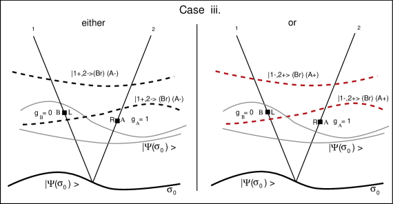
Figure 4: The dynamics of the system of two entangled particles in the relativistic toy model of section. 7 when only one apparatus is switched on.

The reader could easily generalize our rules to arbitrary initial states and arbitrary measurement processes. Once more we specify the rules of the game (see Figs. 4 and 5):

- Completeness: the assignement of the initial state (7.6) represents the maximum information one can have about the system.

- The experimental context: along the world lines of the particles, at two space-time points R (at right for particle 2) and L (at left for particle 1) there are two apparatuses A and B (each characterized by three possible internal states r,+,-) devised to measure $\Theta^{(2)}$ and $\Theta^{(1)},$ respectively . Each apparatus can be switched on or off at the experimenter’s free will.

- Dynamics: once more it is nonlinear and stochastic and associates to any space-like surface in the future of $\sigma_{0}$ a precise statevector according to rules which are the natural generalization of those of Section (7.2) (as before we denote by $V(\sigma,\sigma_{0})$ the space-time volume enclosed by the two indicated surfaces):

i. If

$$\left\{\left[R\notin V(\sigma,\sigma_{0})\right]\vee\left[g_{A}=0\right]\right\}\wedge\left\{\left[L\notin V(\sigma,\sigma_{0})\right]\vee\left[g_{B}=0\right]\right\},$$ (7.7)

then the state ${|}\Psi(\sigma)>$ associated to the surface $\sigma$ is

$$|\Psi(\sigma)>=|\Psi(\sigma_{0})>.$$ (7.8)

This situation occurs for the space-like surfaces represented by continuous lines in Fig.5.

ii. If

$$\left\{\left[R\notin V(\sigma,\sigma_{0})\right]\vee\left[g_{A}=0\right]\right\}\wedge\left\{\left[L\in V(\sigma,\sigma_{0})\right]\wedge\left[g_{B}=1\right]\right\},$$ (7.9)

then the state is

$$either\qquad|\Psi(\sigma)>=|1+,2->\qquad or\qquad|\Psi(\sigma)>=|1-,2+>,$$ (7.10)

the two alternatives occurring at random with equal probabilities.

iii. If

$$\left\{\left[R\in V(\sigma,\sigma_{0})\right]\wedge\left[g_{A}=1\right]\right\}\wedge\left\{\left[L\notin V(\sigma,\sigma_{0})\right]\vee\left[g_{B}=0\right]\right\},$$ (7.11)

then the state is

$$either\qquad|\Psi(\sigma)>=|1+,2->\qquad or\qquad|\Psi(\sigma)>=|1-,2+>,$$ (7.12)

the two alternatives occurring at random with equal probabilities. This situation occurs for the space-like surfaces represented by dashed lines in Fig.4.

iv. Finally if

$$\left\{\left[R\in V(\sigma,\sigma_{0})\right]\wedge\left[g_{A}=1\right]\right\}\wedge\left\{\left[L\in V(\sigma,\sigma_{0})\right]\wedge\left[g_{B}=1\right]\right\},$$ (7.13)

then the state is

$$either\qquad|\Psi(\sigma)>=|1+,2->\qquad or\qquad|\Psi(\sigma)>=|1-,2+>,$$ (7.14)

the two alternatives occurring at random with equal probabilities. This case is represented by the gray dashed lines of Fig.5.

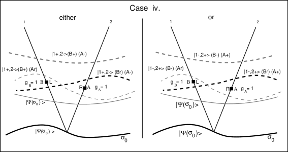
Figure 5: The dynamics of the system of two entangled particles in the relativistic toy model of section. 7 when both apparatuses are switched on.

We have depicted in Fig. 4 the two alternatives corresponding to case iii, and in Fig. 5 those corresponding to case iv. It has to be stressed that the two occurrences in cases ii. and iii. (when only one apparatus is on) have no relations with the corresponding ones of case iv. In fact, leaving aside the case in which no measurement occurs, it has to be stressed that since in the actual world either one or both apparatuses are switched on, and the outcomes are genuinely stochastic, there is no definite relation between the two cases of Fig.4 and of Fig.5 . On the other hand, in case iv., if one considers a space-like surface, like the black dashed lines of Fig.5, passing below one of the two points where there is an apparatus and above the other one, and one supposes that one of the two alternatives has occurred, then the subsequent evolution must be consistent with the chosen alternative, i.e., for all space-like surfaces in the future of both A and B, the statevector of the system remains the same and the previously untriggered apparatus simply registers the property possessed by the microsystem. In this way the necessary requirement that in any case one can consistently describe the evolution from $\sigma_{0}$ to $\sigma_{1}$ and then the one from $\sigma_{1}$ to $\sigma_{2}$ is satisfied.

7.5 Some features of the two-particle model

The model we have just introduced has many interesting features. It contains precise dynamical rules for assigning to each space-like surface in the future of the surface defining the initial conditions a definite statevector. The model is fundamentally stochastic so that, when various alternatives can occur, they occur genuinely at random but in accordance with precise probabilistic laws. The macroscopic apparata are always in definite states (i.e. they always possess definite macroscopic properties) and, for those apparata which are switched on and for space-time points following (on their world lines) the event ”the microsystem triggers the apparatus”, they match the eigenvalues of the observables they are devised to measure. In all other instances, they correspond to their initial untriggered states.

The physical implications of the model obviously agree with those of SQM. In fact, since taken any objective space-time point (after the system-apparatus interaction) on the world line of an apparatus the apparatus state is precisely defined, we can make reference to these states to “read” the outcomes of the process.

Concerning its formal structure it has to be stressed that the model is entirely formulated in a coordinate-free language and thus it satisfies the relativistic requirements [2] of a stochastically Lorentz invariant theory. In fact the statement that an objective space-time point (the one in which there is an apparatus which is on) belongs or does not belong to a precisely defined space-time volume is frame independent and the internal degrees of freedom are assumed to be Lorentz scalars. If we consider the correlations between outcomes, we see that when both apparatuses are switched on they register either (A+) (B-) or (A-) (B+) with equal probabilities and they never register the same outcome. Consequently the model reproduces the perfect correlations of SQM for isospin measurements along the same direction in the isospin singlet state.

The model satisfies the completeness requirement by assumption: there is no better specification of the initial state than the one given by $|\Psi(\sigma_{0})>,$ and its knowledge specifies everything about the future of the system exception made for the actual outcomes of processes whose probability of occurence is fundamentally nonepistemic.

Due to the fact that the model guarantees the perfect correlations of outcomes at the two wings of the apparatus it violates Bell’s locality requirement. It is quite important to stress that:

a). The model exhibits Parameter Independence. In fact, denoting by $P_{S}(+1|g_{R}=\alpha)$ the probability that the outcome at $S$ (taking the values $L$,$R$) be $i$ (taking the values +1,–1) when the apparatus at $S*$ (taking the value $R$ when $S=L$ and $L$ when $S=R$) is switched off ($g_{S*}=0$ ) or it is on ($g_{S*}=1$ ), we have:

$$P_{L}(+1|g_{R} = 1)=P_{L}(+1|g_{R}=0)=\frac{1}{2}$$ (7.15)

$$P_{L}(-1|g_{R} = 1)=P_{L}(-1|g_{R}=0)=\frac{1}{2}$$

and, analogously:

$$P_{R}(+1|g_{R} = 1)=P_{R}(+1|g_{R}=0)=\frac{1}{2}$$ (7.16)

$$P_{R}(-1|g_{R} = 1)=P_{R}(-1|g_{R}=0)=\frac{1}{2}$$

b). The model violates Outcome Independence since the outcomes are perfectly correlated in spite of the fact that they have probability 1/2 of being +1 or -1.

7.6 Events in the two-particle case

At this point the reader should already have perfectly clear all the implications of the model. Suppose one is interested in an event concerning a space-time point $P$ of the world line of the i-th microcostituent of the composite system. The situation can be summarized as follows:

• No one of the space-time points $R$ and/or $L$ at which an apparatus is switched on belongs to the volume $\widetilde{V}(\sigma(P),\sigma_{0})$ lying between $\sigma_{0}$ and $\sigma(P)$ (this last surface being the one defined in section 6). Then the event “the observable $\Theta^{(i)}$ is indefinite” is true.

• If any one of the space-time points $R$ and/or $L$ at which an apparatus is switched on belongs to $\widetilde{V}(\sigma(P),\sigma_{0})$ then the corrisponding event is “the microproperty related (or anticorrelated) to the outcome of the isospin component which has been measured” is definite. The probability of its value is precisely determined by the theory, the actual occurence of one of the possible outcomes is a genuinely random event.

Note that, in accordance with the above statements and when the apparatus at $R$ is on, the assertion “the observable $\Theta^{(1)}$ of particle $1$ is indefinite” holds for all space-time points of the world line of microsystem 1 preceeding the point in which the future light cone from $R$ intersects its world line. The event “the property of microcostituent 1 is definite and it is opposite to the outcome of the measurement at $R$ on system 2” emerges when system 1 reaches the future light cone of the measurement event.

Suppose now one is interested in the event characterizing a precise space-time point of the world line of a macroscopic measuring apparatus. As already remarked and as it should be evident by our argument the event for such a system is always precisely defined and it corresponds to one of the alternatives “the pointer points to the $r$ (ready) position, it points to +, it points to -”. It is important to stress that this holds for both world lines of the apparata independently of the fact that they are switched on or off (in which case they are always in the $r$ state) and independently of the fact that only one or both of them are switched on. In spite of this fact, in the case in which both apparatuses are on, the “definite events” referring to space-time points following, on their world lines, the objective space-time points at which the system-apparatus interactions take place are always opposite, i.e., the perfect anticorrelations characterizing SQM predictions are respected.

7.7 Counterfactuals and nonlocality

We consider it appropriate to call the attention of the reader on the extremely relevant implications of the nonlocal nature of quantum theory for counterfactual arguments within a relativistic context. We recall, first of all, that we have related the possibility of making counterfactual assertions about an objective space-time point to the consideration of the past light cone from the considered point. This is unavoidable within a context like the present one in which the dynamics is fundamentally irreversible, so that the absolute past plays a basic role for any consideration concerning the absolute future.

In this subsection we want to analyze in greater details the problems which are specifically related to nolocality, to have the opportunity of stressing some subtle points. We start by considering a quite simple objection to our way of dealing with counterfactual assertions which could be raised by a naive reader: in the two particle case of subsections 7.4 and 7.6, why an observer who is on the world line of particle 2 at a point Q in the immediate future of the point $R$ at which the isospin component $T_{2z}$ of this particle has been measured (and found, e.g. to have the value –1) is not allowed to make the statement “if an apparatus were switched on on the world line of particle 1 at a point L which is space-like with respect to both $R$ and $Q,$ such an apparatus would register with certainity the outcome +1”? Here is where nonlocality enters. To claim that the above statement is appropriate means to assume that the accessibility sphere from the actual world is represented by all those worlds in which the antecedent, i.e., the fact that the outcome at R has been –1, is true. If the theory were local, i.e. if the outcome at a given point were totally independent from all what is going on at space-like separations, then the argument would be perfectly correct. But, as we know, this is not the case. To allow the reader to grasp this subtle point as well as the argument we will present below, we invite him to consider the three following situations and the related statements:

• We consider an actual world in which everything is like in the two particle case of subsection 7.4 and, moreover, both apparatuses are on. We also consider an observer along the world line of particle 2 immediately after the point $R,$ who is aware of the outcome of the measurement and is also aware of the fact that the apparatus at $L$ is on. Then he can argue in the following way: I know that the apparatus $A$ (the one at $R$) has registered “the isospin has the value –1”, I also know that another apparatus is on at $L$ and that the theory guarantees that the final outcomes are always anticorrelated. I can then claim that the apparatus $B$ at $L$, at any instant following (on its world line) the one of its interaction with particle 1, registers the value +1.

Note that the above is not a counterfactual argument since it makes exclusive reference to the actual world. Moreover, as it should be clear from our analysis in the previous sections, such an argument is perfectly legitimate and correct.

• We consider now the same situation, but we assume that, in the actual world, the apparatus at $L$ is off (note that this is a statement about a precise space-time event, meaning that the apparatus is off when the particle might trigger it). Let us consider once more our observer and his reasoning: I know that the apparatus $A$ at $R$ has registered “the isospin has the value –1” and I also know that the theory guarantees that if two apparata were present and switched on at L and R their outcomes would be perfectly anticorrelated. I can then claim that if the apparatus at $L,$ were on, at any instant following (on its world line) the one of its interaction with particle 1, it would register the value +1.

This, as the reader has certainly clear, is a genuinely counterfactual argument and, according to our criterion (but as we will show, completely in general, due to the nonlocal character of the theory) is definitely illegitimate.

• The final case is exactly the same as the previous one, and, in particular, the apparatus at $L$ is switched off. The only difference consists in the statement made by the observer. Such statement does not refer to a point which is space-like with respect to him, but to one, let us say $T,$ along the world line of particle 1 lying in the future light cone of the observer. The he can claim: I know that the apparatus at $R$ has registered “the isospin has the value –1” and I also know that the theory guarantees that the outcomes of pairs of apparata at R and T (which are time-like separated) are always anticorrelated. So, in spite of the fact that in the actual world no apparatus is on along the world line of particle 1, I can claim (which, for time–like separations also means predict) that if such an apparatus were on at $T,$ then it would register the outcome “the isospin equals $+1$”.

We stress that this is a genuinely counterfactual argument and we also stress that, according to our criterion and to standard wisdom, is a perfectly legitimate one.

To further clarify why the position analyzed in the second of the above cases is inappropriate and to show that the fundamental reason for this derives from the basically nonlocal nature of physical processes which has been so appropriately brought to the attention of the scientific community by the analysis of J.S. Bell [18], we will consider now an hypothetical (and certainly possible) deterministic completion of our toy model, i.e. a nonlocal deterministic hidden variable theory equivalent to it. The theory will be characterized by hidden variables which can take values from a set $\Lambda$ and whose knowledge would unambiguously determine all outcomes of all conceivable measurement processes.

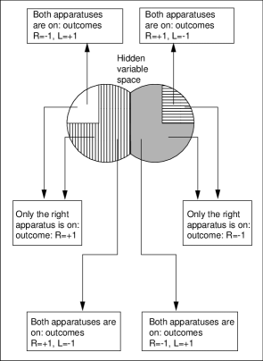
Figure 6: A diagram illustarting, with reference to an hypothetical relativistic and nonlocal hidden variable mode, the problems one has to face when resorting to counterfactual reasoning.

Within the set $\Lambda$ we identify (Fig.6) two subsets $\Lambda_{1}(2,+)$ and $\Lambda_{1}(2,-)$ such that in the case in which only the apparatus at $A$ is switched on, if the actual value $\lambda$ of the hidden variable belongs to $\Lambda_{1}(2,+)$ [$\Lambda_{1}(2,-)]$ then the outcome of the measurement is $+1$ ($-1).$ Let us now consider the case in which both apparatuses are switched on. Then the fact that locality is violated implies that there exist a non empty subset $\Lambda_{1-2}$ of $\Lambda_{1}(2,+)$ such that, for $\lambda\in\Lambda_{1-2}$ the outcome at $A$ is –1 and the one at $B$ is +1 .

To judge of the validity of a counterfactual statement like “if besides the apparatus at $R$ also the apparatus at $L$ were on then the outcome at $L$ would be …” one has to identify the accessibility sphere from the actual world. Which is the appropriate criterion to characterize the worlds which are nearest to the actual one? If one claimed that they are those characterized by the same value of the hidden variables, then for the subset $\lambda\in\Lambda_{1-2}$ of $\Lambda_{1}(2,+)$ the appropriate specification which must replace the dots in the previous sentence would be “$+1$” (while the outcome at $R$ should be characterized by the value opposite to the one which occurs with certainty when only such apparatus is on). On the contrary, if one took the position that the worlds which are nearest to the actual one are those in which the outcome at $R$ is the same as the one obtained in the actual world, then one would be including alternative worlds characterized by a value of the hidden variables belonging to an appropriate subset of $\Lambda_{1}(2,-)$, i.e. worlds such that if only the apparatus at $R$ were on would give the outcome opposite to the one which has occurred in the actual world.

This elementary example should have made clear how delicate is the handling of counterfactual statements in a relativistic nonlocal context and why the prescription we have adopted is the only consistent and logical one. For a further discussion of this delicate point we refer the reader to ref.[4].

8 Relativistic dynamical reduction and local measurements of nonlocal observables

In this section, with reference to our toy model, we will reconsider the experimental set-up of section 3 devised to measure nonlocal observables of a two particle system by resorting to local interactions and detections. The first important remark is that the dynamical evolution has to be enriched (with respect to the examples analyzed in the previous section) to take into account the further interaction processes between the microprobes ([3], [2*], [4*] and [6], [4*], [6*]) and the microscopic constituents ((1) and (2)). Just because these interactions involve only microscopic systems they do not give rise to reduction processes and are accounted by the linear and deterministic evolution summarized in eqs. (3.15)-(3.18). Obviously, also such interactions occur at precise, objective space-time points, so that the whole processs is perfectly covariant.

The first appropriate step is to analyze the evolution from the initial space-like surface $\sigma_{0}$ to a surface $\sigma_{1}$ which has ”crossed” a region in which the interactions between the probes and the particles occur (see Fig. 7, where the considered region is the one at right, lying on the world line of particle 2).

We still assume that the initial state is the singlet isospin state. In order to evaluate the evolution due to the interactions of particle 2 with the probe particles [6], [4*] and [6*] we remark that such an evolution is governed by the appropriate part of the operator $U=\widetilde{U_{z}}U_{y}U_{z}$ defined after eq.(3.13). Such an operator can be written as the direct product of an operator acting on particle 2 and one acting on particle 1 (this expresses the local nature of the interactions with the probes):

$$U=U^{(1)}\otimes U^{(2)},$$ (8.1)

$$U^{(2)}=[P_{z+}^{(2)}P_{L}^{(6)}+P_{z-}^{(2)}P_{R}^{(6)}]\cdot[P_{y+}^{(2)}P_{L}^{(4^{*})}+P_{y-}^{(2)}P_{R}^{(4^{*})}]\cdot[P_{z+}^{(2)}P_{R}^{(6^{*})}+P_{z-}^{(2)}P_{L}^{(6^{*})}].$$

According to eq. (8.1), the effect of applying $U^{(2)}$ to the singlet state is (as one proves by a rather involved calculation):

$$|\Psi(\sigma_{1})>\equiv U^{(2)}|Singlet>|\phi>$$ (8.2)

$$=\frac{i}{2\sqrt{2}}\left(P_{R}^{(6)}|\phi>_{3,6}\right)\left[\left(P_{R}^{(4^{*})}-P_{L}^{(4^{*})}\right)|\phi>_{2^{*},4^{*}}\right]\left(P_{L}^{(6^{*})}|\phi>_{3^{*},6^{*}}\right)|\uparrow_{1z},\uparrow_{2z}>$$

$$+\frac{1}{2\sqrt{2}}\left(P_{R}^{(6)}|\phi>_{3,6}\right)\left[\left(P_{R}^{(4^{*})}+P_{L}^{(4^{*})}\right)|\phi>_{2^{*},4^{*}}\right]\left(P_{R}^{(6^{*})}|\phi>_{3^{*},6^{*}}\right)|\uparrow_{1z},\downarrow_{2z}>$$

$$-\frac{1}{2\sqrt{2}}\left(P_{L}^{(6)}|\phi>_{3,6}\right)\left[\left(P_{L}^{(4^{*})}+P_{R}^{(4^{*})}\right)|\phi>_{2^{*},4^{*}}\right]\left(P_{L}^{(6^{*})}|\phi>_{3^{*},6^{*}}\right)|\downarrow_{1z},\uparrow_{2z}>$$

$$-\frac{i}{2\sqrt{2}}\left(P_{L}^{(6)}|\phi>_{3,6}\right)\left[\left(P_{L}^{(4^{*})}-P_{R}^{(4^{*})}\right)|\phi>_{2^{*},4^{*}}\right]\left(P_{R}^{(6^{*})}|\phi>_{3^{*},6^{*}}\right)|\downarrow_{1z},\downarrow_{2z}>.$$

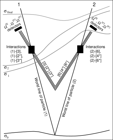
Figure 7: Possible space-like surfaces which is interesting to consider in the case of a nonlocal measurement of the square of the total isospin of a system of two far-away particles.

Recalling the effect of the operators $P_{L}^{(i)}$ and $P_{R}^{(i)}$ on the states $|\phi>_{r,i}:$

$$P_{L}^{(i)}|\phi>_{r,i}=\frac{1}{\sqrt{3}}\left[|0,-1>_{r,i}+|1,1>_{r,i}+|-1,0>_{r,i}\right]$$ (8.3)

$$P_{R}^{(i)}|\phi>_{r,i}=\frac{1}{\sqrt{3}}\left[|0,1>_{r,i}+|1,0>_{r,i}+|-1,-1>_{r,i}\right]$$

we can rewrite the above state (8.2) as:

$$|\Psi(\sigma_{1})\rangle\equiv U^{(2)}|Singlet>|\phi>=$$ (8.4)

$$\frac{1}{6\sqrt{6}}[i|A>|\uparrow_{1z},\uparrow_{2z}>+|B>|\uparrow_{1z},\downarrow_{2z}>-|C>|\downarrow_{1z},\uparrow_{2z}>-i|D>|\downarrow_{1z},\downarrow_{2z}>],$$

where the probe states $|A>,$ $|B>,$ $|C>$ and $|D>$ are given by:

$$|A> = \left(|0,1>_{3,6}+|1,0>_{3,6}+|-1,-1>_{3,6}\right)\otimes$$

$$[|0,1>_{2^{*},4^{*}}+|1,0>_{2^{*},4^{*}}+|1,-1>_{2^{*},4^{*}}-|0,-1>_{2^{*},4^{*}}-|1,1>_{2^{*},4^{*}}-|-1,0>_{2^{*},4^{*}}]\otimes$$

$$\left(|0,-1>_{3^{*},6^{*}}+|1,1>_{3^{*},6^{*}}+|-1,0>_{3^{*},6^{*}}\right),$$

$$|B> = \left(|0,1>_{3,6}+|1,0>_{3,6}+|-1,-1>_{3,6}\right)\otimes$$

$$[|0,1>_{2^{*},4^{*}}+|1,0>_{2^{*},4^{*}}+|1,-1>_{2^{*},4^{*}}+|0,-1>_{2^{*},4^{*}}+|1,1>_{2^{*},4^{*}}+|-1,0>_{2^{*},4^{*}}]\otimes$$

$$\left(|0,1>_{3^{*},6^{*}}+|1,0>_{3^{*},6^{*}}+|-1,-1>_{3^{*},6^{*}}\right),$$

$$|C> = \left(|0,-1>_{3,6}+|1,1>_{3,6}+|-1,0>_{3,6}\right)\otimes$$

$$[|0,1>_{2^{*},4^{*}}+|1,0>_{2^{*},4^{*}}+|1,-1>_{2^{*},4^{*}}+|0,-1>_{2^{*},4^{*}}+|1,1>_{2^{*},4^{*}}+|-1,0>_{2^{*},4^{*}}]\otimes$$

$$\left(|0,-1>_{3^{*},6^{*}}+|1,1>_{3^{*},6^{*}}+|-1,0>_{3^{*},6^{*}}\right),$$

$$|D> = \left(|0,-1>_{3,6}+|1,1>_{3,6}+|-1,0>_{3,6}\right)\otimes$$

$$[|0,-1>_{2^{*},4^{*}}+|1,1>_{2^{*},4^{*}}+|-1,0>_{2^{*},4^{*}}-|0,1>_{2^{*},4^{*}}-|1,0>_{2^{*},4^{*}}-|1,-1>_{2^{*},4^{*}}]\otimes$$

$$\left(|0,1>_{3^{*},6^{*}}+|1,0>_{3^{*},6^{*}}+|-1,-1>_{3^{*},6^{*}}\right).$$

We consider now the further evolution from $\sigma_{1}$ to $\sigma_{2}.$ In this process a micro-macro interaction between the probe particles and the detectors $\Omega^{[6]},$ $\Omega^{[4^{*}]}$ and $\Omega^{[6^{*}]}$ takes place and leads almost immediately to precise locations of their macroscopic pointers. From the above equations we see that all possible triplets of oucomes can occur. Just to fix our mind, let us suppose that reduction has lead to the three outcomes $\Omega^{[6]}=0,$ $\Omega^{[4^{*}]}=0$ and $\Omega^{[6^{*}]}=0.$ The state after the completion of this process is:

$$|\Psi(\sigma_{2})>=$$ (8.9)

$$\frac{N}{6\sqrt{6}}\{i\left[|1,0>_{3,6}\otimes\left(|1,0>_{2^{*},4^{*}}-|-1,0>_{2^{*},4^{*}}\right)\otimes|-1,0>_{3^{*},6^{*}}\right]\otimes|\uparrow_{1z},\uparrow_{2z}>$$

$$+\left[|1,0>_{3,6}\otimes\left(|1,0>_{2^{*},4^{*}}+|-1,0>_{2^{*},4^{*}}\right)\otimes|-1,0>_{3^{*},6^{*}}\right]\otimes|\uparrow_{1z},\downarrow_{2z}>$$

$$-\left[|-1,0>_{3,6}\otimes\left(|1,0>_{2^{*},4^{*}}+|-1,0>_{2^{*},4^{*}}\right)\otimes|-1,0>_{3^{*},6^{*}}\right]\otimes|\downarrow_{1z},\uparrow_{2z}>$$

$$-i\left[|-1,0>_{3,6}\otimes\left(|-1,0>_{2^{*},4^{*}}-|1,0>_{2^{*},4^{*}}\right)\otimes|1,0>_{3^{*},6^{*}}\right]\otimes|\downarrow_{1z},\downarrow_{2z}>,$$

$N$ being a normalization factor.

And now comes the final step. We consider the subsequent evolution to a final state which is associated to a space-like surface in the future of $\sigma_{2},$ obtained by crossing the region of Fig. 7 where the interactions of particle 1 with the probe particles takes place (subsequently the detectors at left will simply register the definite situation of the probes). Such evolution is governed by the unitary operator $U^{(1)}$ which has the same form as $U^{(2)}$ of eq. (8.1) with the apices [3], [2*] and [3*] replacing [6], [4*] and [6*]. With a rather tedious calculations one gets the result:

$$|\Psi(\sigma_{final})>=\left[|0,0>_{3,6}\otimes|0,0>\otimes|0,0>_{3^{*},6^{*}}\right]\otimes|Singlet>.$$ (8.10)

Obviously, one can perform the calculation by assuming any other possible set of outcomes of the detectors at the right wing. For instance, if one chooses the set $\Omega^{[6]}=1,$ $\Omega^{[4^{*}]}=0$ and $\Omega^{[6^{*}]}=0$ and goes through precisely the same calculation, one gets, in place of eq. (8.10) the following one:

$$|\Psi(\sigma_{final})>=\left[|-1,1>_{3,6}\otimes|0,0>\otimes|0,0>_{3^{*},6^{*}}\right]\otimes|Singlet>.$$ (8.11)

As expected, the final state of the system is always the singlet and the states of the various pairs of apparata appearing in it are such that the sum of their eigenvalues is always zero, as it must be in order that the formalism be internally consistent. The same happens for different initial states and for any possible choice of the outcomes at the right wing. We believe that this simple exercise should have made clear to the reader the elegance and the logical coherence of the formalism.

Obviously, mastering completely the theoretical scheme allows us to tackle, also in the more general case of nonlocal measurements, the problem of property attribution to the system. Since such measurements involve a pair of space-time points one has to identify the space-like hypersurface which has to be considered for drawing the relevant conclusions. According to our criterion, such a hypersurface is the boundary of the two past light cones from the pair of points one is taking into account on the world lines of the two particles. It is then obvious that, if consideration is given to a pair of points which preceed the two interaction regions (both at right and at left) of the particles with the probes, the theory associates to such a surface the singlet state and one can claim that “the composite system possesses the objective property of having total isospin equal to 0”. Such an assertion is confirmed by the subsequent measurement procedure and the communication between the two obserbers concerning the outcomes they have registered. On the contrary, if one considers a pair of points such that one follows and the other one preceeds the particle-probe interactions, i.e. two points like those in which the hypersurface $\sigma_{1}$ of Fig. 7 crosses the two world lines, the state describing the overall situation is the one of eq.(8.2) for which the square of the total isospin is undefined. One can go on reasoning in the just outlined way. We have no space to discuss all aspects of such a procedure in detail, we simply point out that, with the chosen criterion the unfolding of the process and the statements one is led to make are quite natural.

The last comment which is worth making concerns the other possible (in principle) choice for the space-like surface one uses to identify the possessed properties. As already remarked, one could make reference to the future rather than to the past light cone without meeting any logical contradiction. However, we cannot avoid stressing that the ensuing picture is rather peculiar. The reasons should be quite obvious: in order to speak of an objective situation at an objective space-time point it is much more natural to make reference to its absolute past than to the past plus the whole region which is space-like with respect to it. In particular, we point out that when the future light cone criterion is adopted, in the situation of section 7.4 and in the case in which only the apparatus at $R$ is switched on, the isospin of particle 1 becomes definite at the space-time point at which the past light cone from $R$ intersects its world line. In our opinion, this sort of (luminal) backward causation is less natural than the forward one implied by the alternative criterion. Even more peculiar aspects emerge when one takes into account nonlocal measurements. These reasons make our choice, whith its precise physical implications, definitely preferable.

9 Conclusions

The detailed analysis we have performed should, in our opinion, have made clear the conceptually most relevant features that any relativistic model of dynamical reduction must satisfy. It should also have made clear that the relativistic generalizations of CSL satisfy, in principle, all requirements we have identified. As already mentioned, such models encounter some technical difficulties. But we believe that the present analysis makes plausible that the main physical ideas at the basis of the considered approaches must be essential ingredients of any attempt to account for the macro-objectification process respecting the relativistic requirements and emboding the fundamental nonlocal aspects of natural processes.

References

- [1] P. Pearle, in: Sixty-Two Years of Uncertainity, A. Miller (Ed), New York, Plenum Press, 1990.
- [2] G.C. Ghirardi, R. Grassi and P. Pearle, Found. Phys., 20, 1271 (1990).
- [3] G.C. Ghirardi, R. Grassi and P. Pearle, in: Symposium on the Foundations of Modern Physics 1990, P. Lahti and P. Mittelstaedt, (Eds.), World Scientific, Singapore, 1991.
- [4] G.C. Ghirardi and R. Grassi, Stud. Hist. Philos. Sci., 25, 97 (1994).
- [5] G.C. Ghirardi, Found. Phys. Lett., 9, 313 (1996).
- [6] G.C. Ghirardi, in: Open Systems and Measurement in Relativistic Quantum Theory, H.P. Breuer and F. Petruccione, (Eds.), Springer, Berlin, 1999.
- [7] H.P. Breuer and F. Petruccione, in: Open Systems and Measurement in Relativistic Quantum Theory, H.P. Breuer and F. Petruccione, (Eds.), Springer, Berlin, 1999.
- [8] Y. Aharonov and D.Z. Albert Phys. Rev. D 24, 359 (1981).
- [9] Y. Aharonov and D.Z. Albert Phys. Rev. D 21, 3316 (1980).
- [10] Y. Aharonov and D.Z. Albert Phys. Rev. D 29, 228 (1984).
- [11] K.-E. Hellwig and K. Kraus, Phys. Rev. D 1, 566 (1970).
- [12] L. Laundau and R. Peierls, Z. Phys., 69, 56 (1931).
- [13] S. Tomonaga, Progr. Theor. Phys., 1, 27 (1946), J. Schwinger, Phys. Rev., 74 1439 (1948).
- [14] G.C. Ghirardi, A. Rimini and T. Weber, Phys. Rev. D 34, 470 (1986).
- [15] J.S. Bell in: Scroedinger. Centenary celebration of a polymath, C.W. Kilmister (Ed.), Cambridge University Press, Cambridge, 1987.
- [16] P. Pearle, Phys. Rev. A 39, 2277 (1989).
- [17] G. C. Ghirardi, P. Pearle and A. Rimini, Phys. Rev. A 42, 78 (1990).
- [18] J.S. Bell, Physics 1, 195 (1964).