Quantum theory of self-action of ultrashort light pulses
in an inertial nonlinear medium

Abstract

The systematic theory of the formation of the short light pulses in the squeezed state during the propagation in a medium with inertial Kerr nonlinearity is developed. The algebra of time-dependent Bose-operators is elaborated and the normal-ordering theorem for them is formulated. It is established that the spectral region where the quadrature fluctuations are weaker than the shot-noise, depends on both the relaxation time of the nonlinearity and the magnitude of the nonlinear phase shift. It is also shown that the frequency at which suppression of the fluctuation is greatest can be controlled by adjusting the phase of the initial coherent light pulse. The spectral correlation function of photons is introduced and photon antibunching is found.

]

I INTRODUCTION

During the past years the study of formation of nonclassical light pulses in nonlinear media has been the focus of a considerable attention. The present article is devoted to the development of the consecutive theory of formation of nonclassical short light pulses in nonlinear media with inertial Kerr nonlinearity. It is well known, that in nonlinear media in the presence of the self-action effect the squeezing of quantum fluctuations of one quadrature component of a field with conservation of the photon statistics take place [1]. At present there are two basic directions of research in the quantum theory of self-action of ultrashort light pulses (USPs). In the first approach [2, 3, 4, 5] the calculations of the nonclassical light formation at the self-action of light pulses assume that the nonlinear response of nonlinearity is instantaneous and that the relative fluctuations are small. This latter assumption is valid for the intensive USPs frequently used in experiments. However, a finite relaxation time of the nonlinearity has a principled importance as the relaxation time determines the region of the spectrum of the quantum fluctuation below the standard noise level. For the first time, in [6] was noted that for the correct quantum solution of self-action, it is necessary to take into account the presence of quantum noise. The presence of quantum noise was anticipated in [7] as thermal addition to the interaction Hamiltonian. This addition was necessary in order to satisfy the commutation relation for time-dependent Bose-operators. If the interaction Hamiltonian has the normally ordered form [8] then it is not necessary to have deal with thermal fluctuations. This approach allows us to develop an algebra of time-dependent Bose-operators and to investigate the spectrum of quantum fluctuations of the quadrature components. The results of the quantum theory of self-action for USPs in the medium with the relaxation Kerr nonlinearity based on the normally ordered interaction Hamiltonian and the developed algebra of time-dependent Bose-operators are presented below.

II THE QUANTUM EQUATION OF SELF-ACTION OF USPs

For the monochromatic radiation the quantum equation of self-action can be found, for example, in [5]. Up to now, the proper quantum equation of the self-action for USPs with the account of relaxation behavior of the nonlinearity is absent in the literature. It is necessary to mention that the deduction of the quantum equation is based on the interaction Hamiltonian. However, in this case we obtain the time-evolution equation for the Bose-operators. For monochromatic radiation the conversion of time-evolution equation into space-evolution one is done using the $t\smash{\longrightarrow}z/u$ replacement, where $z$ is time variable and $u$ is the speed of pulse in nonlinear media. If we deal with the propagation of pulse in nonlinear media then the ”impulse operator” of a pulse field should be used [9]. We begin with the analyse of the self-action of UPSs in non-inertial nonlinear media.

A THE QUANTUM EQUATION OF SELF-ACTION IN THE NON-INERTIAL NONLINEAR MEDIA

In nonlinear media with non-inertial behavior the self-action process is described using the impulse operator (quantity of movement) $\hat{G}_{int}(z)$ [7]

$$\hat{G}_{int}(z)=\beta\hbar\!\!\int_{-\infty}^{\infty}\!\!\hat{\mathbf{N}}[\hat{n}^{2}(t,z)]dt,$$ (1)

where $\hat{\mathbf{N}}$ is the operator of normal ordering, factor $\beta$ is defined by the cubic nonlinearity of the medium [5]. In consequence, in the Heisenberg representation the quantum space-evolution equation for the annihilation photons Bose-operator in a given cross section $z$ ($\hat{A}(t,z)$) has the form

$$-i\hbar\frac{\partial\hat{A}(t,z)}{\partial z}=\left[\hat{A}(t,z),\hat{G}_{int}(z)\right].$$ (2)

In agreement with (1) the quantum equation of self-action for a light pulse follows from (2)

$$\frac{\partial\hat{A}(t,z)}{\partial z}-i\beta\hat{A}^{+}(t,z)\hat{A}^{2}(t,z)=0.$$ (3)

Eq.(3) is written in the moving coordinate system: $z\smash{=}z^{\prime}$ and $t\smash{=}t^{\prime}\smash{-}z/u$. It is important to note that in comparison with the so-called nonlinear Heisenberg equation, used in the quantum theory of optical solitons, in (3) the dissipation of light pulse in the nonlinearity is not taken into account. This approach corresponds to the first approximation of dissipation theory. In fact, the traditional way to introduce the quantum equation of self-action is based on the interaction Hamiltonian. In this case one gets the time-evolution equation. The transition to the space-evolution, as already mentioned, is realized using replacement $t\longrightarrow z/u$. This approach is enough reasonable in case the radiation is monochromatic. If we deal with the nonlinear propagation of a pulse, we use the impulse operator of a pulse field (1) which is connected with the evolution of field in space. Eq.(3) has the solution

$$\hat{A}(t,z)=e^{i\gamma\hat{n}_{0}(t)}\hat{A}_{0}(t),$$ (4)

where $\gamma\smash{=}\beta z$ and, as usual, $\hat{A}_{0}(t)$ is the value of the operator at input of nonlinear media ($\hat{A}_{0}(t)\smash{=}\hat{A}(t,z\smash{=}0)$), $\hat{n}_{0}(t)\smash{=}\hat{A}^{+}_{0}(t)\hat{A}_{0}(t)$ is the photon number “density” operator. For its hermitian conjugated operator we find

$$\hat{A}^{+}(t,z)=\hat{A}^{+}_{0}(t)e^{-i\gamma\hat{n}_{0}(t)}.$$ (5)

In agreement with (4) and (5) the operator $\hat{n}(t,z)=\hat{A}^{+}(t,z)\hat{A}(t,z)$ does not change itself in nonlinear medium:

$$\hat{n}(t,z)=\hat{n}(t,z\smash{=}0)=\hat{n}_{0}(t),$$ (6)

where $z\smash{=}0$ corresponds to the input of the nonlinear medium. In fact, (6) means that the photon statistic in media remains unchanged. The commutation relation at the input ($z\smash{=}0$) of nonlinearity $[\hat{A}_{0}(t_{1}),\hat{A}^{+}_{0}(t_{2})]=\delta(t_{1}\smash{-}t_{2})$, should be satisfied for any coordinate $z$ in nonlinear media:

$$[\hat{A}(t_{1},z),\hat{A}^{+}(t_{2},z)]=\delta(t_{1}-t_{2}).$$ (7)

The solutions (4) and (5) do not permit to verify the commutation relation (7). Besides, the analyse of the statistical characteristics of the pulse is accompanied by the necessity of the reduction to the normally ordered form of the expression $e^{i\gamma\hat{n}_{0}(t)}$. In this case, the solutions (4) and (5) are accompanied by the singularity of the function $\delta(t)$ at $t\smash{=}0$. The specified circumstances represent the main deficiency of the quantum theory of self-action of USPs in non-inertial nonlinear media.

B THE QUANTUM EQUATION OF SELF-ACTION IN THE INERTIAL NONLINEAR MEDIA

In the classical theory, the self-action process in inertial nonlinear media is described by the equation (in the first approximation of the dispersion theory) [5]

$$\frac{\partial B(t,z)}{\partial z}+\frac{1}{u}\frac{\partial B(t,z)}{\partial t}-i\frac{k_{0}}{n_{0}}\Delta n(| B (t,z)|^{2})$$ (9)

$$\times B(t,z)=0,$$

where: $B(t,z)$- the complex amplitude of a pulse, $z$- the distance in the nonlinear media, $u$- the group velocity, $\Delta n(|B(t,z)|^{2})\smash{=}\Delta n((t,z)$- the nonlinear addition to the coefficient of refraction. We consider that the last term of (9) is caused by the high-frequency Kerr effect, and its evolution follows from the equation

$$\tau_{r}\frac{\partial\Delta n(t,z)}{\partial t}+\Delta n(t,z)=\frac{1}{2}\,n_{2}|B(t,z)|^{2}.$$ (10)

Here $\tau_{r}$ represents the relaxation time of the nonlinearity and $n_{2}$- the nonlinear factor. We mention that in general the behaviour of the nonlinear addition differs from the one characterized by (10). However, if the carrying frequency of a pulse is far enough from the resonance and the pulse duration $\tau_{p}$ is greater that the relaxation time $\tau_{r}$, then (10) is correct [5]. The solution of (10) looks like

$$\Delta n(t,z)=(n_{2}/2)\int_{-\infty}^{t}H(t-t_{1})|B(t_{1},z)|^{2}\,dt_{1}.$$ (11)

The function of nonlinear response $H(t)$ is entered in such a way that in the limit $\tau_{p}\smash{\gg}\tau_{r}$ the nonlinear addition becomes $\Delta n(t,z)\smash{=}(n_{2}/2)|B(t,z)|^{2}$. In the moving system of coordinates $(t^{\prime}\smash{=}t\smash{-}z/u,z^{\prime}\smash{=}z)$, taking into account (11), eq. (9) takes the form

$$\frac{\partial B(t,z)}{\partial z}=i\gamma^{\star}\int_{0}^{\infty}H(t_{1})|B(t-t_{1},z)|^{2}\,dt_{1}B(t,z),$$ (12)

where $\gamma^{\star}\smash{=}k_{0}n_{2}/2n_{0}$ and the quotation-marks ( ^′ ) in new system of coordinates further will be lowered for simplicity. The transition to the quantum equation usually is carried out in the spectral representation. However, in the considered case it is more natural to use time representation. We make in (12) replacement of the complex amplitudes with the operators, entered in the previous sections,

$$B(t,z)\rightarrow iC\hat{A}(t,z),\quad B^{*}(t,z)\rightarrow-iC\hat{A}^{+}(t,z).$$ (13)

The right part of the equation we have gotten in this way, will be written below in normally ordered form. In order to take into account the presence of the vacuum fluctuations, existing up to the moment of arrival of the pulse, we will replace in (12) the bottom limit of integration by ${-\infty}$. As a result we get ($C\smash{=}(\hbar\omega_{0}/2V)^{1/2}$, $\beta\smash{=}\gamma^{\star}C^{2}/2$)

$$\frac{\partial\hat{A}(t,z)}{\partial z}=i\beta\int_{-\infty}^{\infty}H(|t_{1}|)\hat{A}^{+}(t\smash{-}t_{1},z) \hat{A}(t\smash{-}t_{1},z)$$ (15)

$$\times\,\hat{A}(t,z)dt_{1}.$$

Eq.(15) represents the correct quantum equation and can be obtained from space evolution equation for the operator $\hat{A}(t,z)$ in interaction representation (2). Taking into consideration the inertial behaviour of the nonlinearity, the impulse operator of a pulse should be introduced as:

$$\hat{G}_{int}(z)=\hbar\beta\int_{-\infty}^{\infty}dt \int_{-\infty}^{t}H(t-t_{1})$$ (17)

$$\times\hat{\mathbf{N}}\left[\,\hat{n}(t,z)\hat{n}(t_{1},z)\right]dt_{1},$$

where $H(t)$ is the nonlinear response of the medium (see (11)) ($H(t)\smash{\neq}0$ at $t\smash{\geq}0$ and $H(t)\smash{=}0$ at $t\smash{<}0$). We note that the integral expression in (17) at the moment of time $t$ depends only on the previous ones. Therefore, in this case the causality principle relative to measured physical value is not broken. An important condition that must be satisfied by the impulse operator is

$$[\hat{G}_{int}(z),\hat{n}(t,z)]=[\hat{G}_{int}(z),\hat{n}_{0}(t)]=0,$$ (18)

which means that the photon number operator remains unchanged in medium (photon number is a constant of motion [1]). The annihilation Bose-operator which agrees with the (17) verifies the equation of self-action

$$\frac{\partial\hat{A}(t,z)}{\partial z}-i\beta q[\hat{n}_{0}(t)]\hat{A}(t,z)=0,$$ (19)

where

$$q[\hat{n}_{0}(t)]=\int_{0}^{\infty}H(t_{1})\left[\,\hat{n}_{0}(t-t_{1})+\hat{n}_{0}(t+t_{1})\right]dt_{1}.$$ (20)

If $H(t)\smash{=}\delta(t)$ then (19) is converted into (3). Eq.(3) can be obtained in the same form if we consider that the response of the nonlinearity has relaxation behaviour $H(t)$ in accordance with (11) and the relaxation time $\tau_{r}$ is significantly less than the duration of a pulse $\tau_{p}$. At the same time, as will be shown further, in this limited case also, the account of finite relaxation time plays the main role in formation of the nonclassical light. It is necessary to note, that by replacement in (19) the operators on complex values we obtain the equation, which not completely coincides with the classical equation of self-action in presence of the non-stationary nonlinear response. There is no second term, included in (20) as $\hat{n}_{0}(t+t_{1})$. The presence of this term in quantum theory, which at the first sight is in contradiction with the causality principle, is connected with the quantum description that even in absence of a pulse the vacuum fluctuations always are present. A response function was introduced already in the model for the Kerr effect by Blow et al. [6]. Although the need for an attendant noise source was anticipated by these authors, they did not indicate where it should be inserted. In [7] the quantum noise as thermal fluctuations was additive inserted in the interaction Hamiltonian but this procedure did not allow to develop the consistent quantum theory of self-action of USPs. According to (17), the operator $\hat{n}(t,z)$ remains unchanged in nonlinear media (see (6)). Solving the spatial evolution equation (19), the annihilation (creation) photons Bose-operators in nonlinear medium have the following form:

$$\hat{A}(t,z) = e^{i\gamma q[\hat{n}_{0}(t)]}\,\hat{A}_{0}(t).$$ (21)

$$\hat{A}^{+}(t,z) = \hat{A}^{+}_{0}(t)\,e^{-i\gamma q[\hat{n}_{0}(t)]}.$$ (22)

In (21) and (22) $\hat{A}_{0}(t)\smash{=}\hat{A}(t,0)$, $\gamma\smash{=}\beta z$. The expression $q[\hat{n}_{0}(t)]$ (see (20)) it is convenient to be written as:

$$q[\hat{n}_{0}(t)]=\int_{-\infty}^{\infty}\!\!h(t_{1})\hat{n}_{0}(t-t_{1})dt_{1},\quad(h(t)=H(|t|).$$ (23)

If we consider $\hat{n}$ to be time-independent, then the expressions (21) and (22) give results for the monochromatic field. In the case that the nonlinear response in (21), (22) has the form $h(t)=\delta(t)$, the results for non-inertial nonlinear media can be obtained (see (5)). To find the statistical characteristics of a pulse at the output of the nonlinear medium it is necessary to estimate the averages of the operators $\hat{A}(t,z)$, $\hat{A}^{+}(t,z)$ and their combinations. They can be estimated, if the operator expressions are given in the normally ordered form, when the creation photons Bose-operators are placed at the left of the annihilation photons Bose-operators. The use of the expressions (21), (22) involves the development of a special mathematical device.

III THE ALGEBRA OF THE TIME-DEPENDENT BOSE-OPERATORS

For the beginning, in order to simplify some expressions we introduce the operators:

$$\hat{O}(t)=i\gamma q[\hat{n}_{0}(t)],\qquad\hat{O}^{+}(t)=-i\gamma q[\hat{n}_{0}(t)],$$ (24)

where $\hat{O}^{+}(t)\smash{=}-\hat{O}(t)$. Hence, the equations of self-action (21), (22) can be represented as:

$$\hat{A}(t,z) = e^{\hat{O}(t)}\,\hat{A}_{0}(t),$$ (25)

$$\hat{A}^{+}(t,z) = \hat{A}^{+}_{0}(t)\,e^{\hat{O}^{+}(t)}.$$ (26)

Taking into account (23), is it easy to remark that

$$[\hat{O}(t_{1}),\hat{O}(t_{2})]=0.$$ (27)

In consequence we have

$$e^{\hat{O}(t_{1})}e^{\hat{O}(t_{2})} = e^{\hat{O}(t_{2})}e^{\hat{O}(t_{1})}$$ (28)

$$= e^{\hat{O}(t_{1})+\hat{O}(t_{2})}=e^{\hat{O}(t_{2})+\hat{O}(t_{1})}.$$ (29)

A THE PERMUTATION OPERATOR RELATIONS

The following operator permutation relations hold:

$$\hat{A}_{0}(t_{1})\hat{O}(t_{2}) = [\hat{O}(t_{2})+i\gamma h(t_{2}-t_{1})]\hat{A}_{0}(t_{1}),$$ (30)

$$\hat{A}_{0}(t_{1})\hat{{O}^{+}}(t_{2}) = [\hat{O}^{+}(t_{2})-i\gamma h(t_{2}-t_{1})]\hat{A}_{0}(t_{1}),$$ (31)

$$\hat{A}^{+}_{0}(t_{1})\hat{O}(t_{2}) = [\hat{O}(t_{2})-i\gamma h(t_{2}-t_{1})]\hat{A}^{+}_{0}(t_{1}),$$ (32)

$$\hat{A}^{+}_{0}(t_{1})\hat{{O}^{+}}(t_{2}) = [\hat{O}^{+}(t_{2})+i\gamma h(t_{2}-t_{1})]\hat{A}^{+}_{0}(t_{1}).$$ (33)

Using the mathematical induction it is possible to demonstrate the validity of the formulae ($m\in N$):

$$\hat{A}_{0}(t_{1})\hat{O}^{m}(t_{2}) = [\hat{O}(t_{2})+i\gamma h(t_{2}-t_{1})]^{m}\hat{A}_{0}(t_{1}),$$ (34)

$$\hat{A}_{0}(t_{1})\hat{{O}^{+}}^{m}(t_{2}) = [\hat{O}^{+}(t_{2})-i\gamma h(t_{2}-t_{1})]^{m}\hat{A}_{0}(t_{1}),$$ (35)

$$\hat{A}^{+}_{0}(t_{1})\hat{O}^{m}(t_{2}) = [\hat{O}(t_{2})-i\gamma h(t_{2}-t_{1})]^{m}\hat{A}^{+}_{0}(t_{1}),$$ (36)

$$\hat{A}^{+}_{0}(t_{1})\hat{{O}^{+}}^{m}(t_{2}) = [\hat{O}^{+}(t_{2})+i\gamma h(t_{2}-t_{1})]^{m}\hat{A}^{+}_{0}(t_{1}).$$ (37)

To simplify the operator algebra is useful to redefine

$$\emph{G}(t_{2}\smash{-}t_{1})\smash{=}i\gamma h(t_{2}\smash{-}t_{1}),\quad\emph{G}^{*}(t_{2}\smash{-}t_{1})\smash{=}-i\gamma h(t_{2}\smash{-}t_{1}).$$ (38)

Decomposing $e^{\hat{O}(t)}$ and $e^{\hat{O}^{+}(t)}$ in Taylor series we obtain the operator permutation relations which play an important role at the estimation of the statistical characteristics of a pulse. Hence, finally we have:

$$\hat{A}_{0}(t_{1})e^{\hat{O}(t_{2})} = e^{\hat{O}(t_{2})+\emph{G}(t_{2}-t_{1})}\hat{A}_{0}(t_{1}),$$ (39)

$$\hat{A}_{0}(t_{1})e^{\hat{O}^{+}(t_{2})} = e^{\hat{O}^{+}(t_{2})+\emph{G}^{*}(t_{2}-t_{1})}\hat{A}_{0}(t_{1}),$$ (40)

$$e^{\hat{O}(t_{1})}\hat{A}^{+}_{0}(t_{2}) = \hat{A}^{+}_{0}(t_{2})e^{\hat{O}(t_{1})+\emph{G}(t_{2}-t_{1})},$$ (41)

$$e^{\hat{O}^{+}(t_{1})}\hat{A}^{+}_{0}(t_{2}) = \hat{A}^{+}_{0}(t_{2})e^{\hat{O}^{+}(t_{1})+\emph{G}^{*}(t_{2}-t_{1})}.$$ (42)

Using the permutation relations (41) it is possible to verify the commutation relation (7) for the operators $\hat{A}(t,z)$ and $\hat{A}^{+}(t,z)$.

B THE NORMAL ORDERING THEOREM

As pointed out previously, in the considered analyse another important question is represented by the reduction to normally ordered form of the operators $\hat{A}(t,z)$ and $\hat{A}^{+}(t,z)$. In (23) we proceed to normalized time $\theta=t_{1}/\tau_{r}$ and then (24) can be presented like:

$$\hat{O}(t) = i\gamma\int_{-\infty}^{\infty}\tilde{h}(\theta)\hat{n}_{0}(t-\theta\tau_{r})d\theta$$ (43)

$$= \int_{-\infty}^{\infty}\emph{G}(\theta)\hat{n}_{0}(t\smash{-}\theta\tau_{r})d\theta,$$ (44)

where $\widetilde{h}(\theta)=\tau_{r}h(\theta\tau_{r})$ and $\emph{G}(\theta)=i\gamma\widetilde{h}(\theta)$. For the reduction of the expressions (24) to the normally ordered form the following theorem can be used:
Theorem:    Bose-operator $e^{\hat{O}(t)}$ can be represented in the normally ordered form this way:

$$e^{\hat{O}(t)}=\hat{\mathbf{N}}\exp{\left\{\int_{-\infty}^{\infty}\left[e^{G(\theta)}-1\right]\hat{n}_{0}(t-\theta\tau_{r})d\theta\right\}}.$$ (45)

The operators in the integral expression may be understood as the $c$-numbers. In [10] the similar theorem in the spectral representation was formulated and demonstrated and we mention only that the similar demonstration can be done also in this case. In fact in [10] the integration limits are not defined and the theorem has not a obvious applicability. The demonstration of (45) does not represent the central objective of this article so we formulate the theorem in the time-representation only. The average value of the $e^{\hat{O}(t)}$ is given by the formula

$$\langle e^{\hat{O}(t)}\rangle=\exp{\left\{\int_{-\infty}^{\infty}\left[e^{G(\theta)}-1\right]\bar{n}_{0}(t-\theta\tau_{r})d\theta\right\}}.$$ (46)

C THE AVERAGE VALUES OF  $e^{\hat{O}(t)}$ AND  $e^{\hat{O}^{+}(t)}$

In most of the experimental situations $\gamma\ll 1$ which allows one to decompose the integral expression in the (46) and to limit decomposition at terms having order $\gamma^{2}$. Using this approach we have:

$$\langle e^{\hat{O}(t)}\rangle=\exp \Bigl{[}\int_{-\infty}^{\infty}\emph{G}(\theta)\bar{n}_{0}(t-\theta\tau_{r})d\theta$$ (48)

$$+\frac{1}{2}\int_{-\infty}^{\infty}\emph{G}^{2}(\theta)\bar{n}_{0}(t-\theta\tau_{r})d\theta\Bigl{]},$$

where $\bar{n}_{0}(t)\smash{=}\langle\hat{n}_{0}(t)\rangle\smash{=}|\alpha_{0}(t)|^{2}$. It is convenient to enter in further analyse the envelope of a pulse $\rho(t)$, so that $\alpha_{0}(t)\smash{=}\rho(t)\alpha_{0}$. If the initial pulse has the gaussian form then $\rho(0)\smash{=}1$. For simplicity we denote:

$$\psi(t)=\gamma\int_{-\infty}^{\infty}\widetilde{h}(\theta)\bar{n}_{0}(t-\theta\tau_{r})d\theta,$$ (49)

$$\mu(t)=\frac{1}{2}\gamma^{2}\!\!\int_{-\infty}^{\infty}\widetilde{h}^{2}(\theta)\bar{n}_{0}(t-\theta\tau_{r})d\theta.$$ (50)

From (48) we have

$$\langle e^{\hat{O}(t)}\rangle=e^{i\psi(t)-\mu(t)},\quad\langle e^{\hat{O}^{+}(t)}\rangle=e^{-i\psi(t)-\mu(t)}.$$ (51)

The parameters $\psi(t)$ and $\mu(t)$ are connected with the self-action effect and $\psi(t)$ represents nonlinear phase addition. Then

$$\psi(t)=\psi_{0}\int_{0}^{\infty}\widetilde{h}(\theta)\rho^{2}(t-\theta\tau_{r})d\theta,$$ (52)

$$\mu(t)=\mu_{0}\int_{0}^{\infty}\widetilde{h}^{2}(\theta)\rho^{2}(t-\theta\tau_{r})d\theta,$$ (53)

where $\psi_{0}=2\gamma\alpha^{2}_{0}=2\gamma\bar{n}_{0}$ and $\mu_{0}=\gamma^{2}\bar{n}_{0}=\gamma\psi_{0}/2$. A special interest is represented by the estimation of the average values of the Bose-operator combinations at coherent initial states (see (24)). Taking into account (24) we have:

$$e^{\hat{O}(t_{1})}e^{\hat{O}(t_{2})}\smash{=}e^{\hat{O}(t_{2})}e^{\hat{O}(t_{1})}\smash{=}e^{\hat{O}(t_{1})+\hat{O}(t_{2})}\smash{=}e^{\hat{Q}(t_{1},t_{2})}.$$ (54)

In consequence we find

$$\hat{\mathbf{N}}\left[e^{\hat{O}(t_{1})}e^{\hat{O}(t_{2})}\right]=\hat{\mathbf{N}}\left[e^{\hat{Q}(t_{1},t_{2})}\right],$$ (55)

where:

$$\hat{Q}(t_{1},t_{2}) = \hat{O}(t_{1})+\hat{O}(t_{2})$$ (56)

$$= \int_{-\infty}^{\infty}\!\!\widetilde{\emph{G}}(t_{1},t_{2};\theta)\hat{n}_{0}(\theta\tau_{r})d\theta,$$ (57)

$$\widetilde{\emph{G}}(t_{1},t_{2};\theta) = i\gamma\widetilde{h}(t_{1}-\theta\tau_{r})+i\gamma\widetilde{h}(t_{2}-\theta\tau_{r}).$$ (58)

Using the theorem of normal ordering for (57) we estimate the averages of different combinations of Bose-operators:

$$\langle e^{\hat{O}(t_{1})+\hat{O}(t_{2})}\rangle = e^{i[\psi(t_{1})+\psi(t_{2})]-\mu(t_{1},t_{2})-\emph{K}(t_{1},t_{2})},$$ (59)

$$\langle e^{\hat{O}^{+}(t_{1})+\hat{O}(t_{2})}\rangle = e^{i[-\psi(t_{1})+\psi(t_{2})]-\mu(t_{1},t_{2})+\emph{K}(t_{1},t_{2})},$$ (60)

$$\langle e^{\hat{O}(t_{1})+\hat{O}^{+}(t_{2})}\rangle = e^{i[\psi(t_{1})-\psi(t_{2})]-\mu(t_{1},t_{2})+\emph{K}(t_{1},t_{2})},$$ (61)

$$\langle e^{\hat{O}^{+}(t_{1})+\hat{O}^{+}(t_{2})}\rangle = e^{-i[\psi(t_{1})+\psi(t_{2})]-\mu(t_{1},t_{2})-\emph{K}(t_{1},t_{2})},$$ (62)

where $\mu(t_{1},t_{2})\smash{=}\mu(t_{1})\smash{+}\mu(t_{2})$ and $\emph{K}(t_{1},t_{2})$ represents the temporal correlator

$$\emph{K}(t_{1},t_{2})=\mu_{0}\int_{-\infty}^{\infty}\widetilde{h}(t_{1}\smash{-}\theta\tau_{r})\widetilde{h}(t_{2}\smash{-}\theta\tau_{r})\rho^{2}(\theta\tau_{r})d\theta.$$ (63)

In agreement with most of the experimental situations the approximation $\tau_{p}\smash{\gg}\tau_{r}$ can be used. In this case in (52),(53) and (63) we can suppose that in time the envelope of a pulse slowly change itself so it practically does not depend on the change of the integration variable. Therefore it is possible to eliminate it from the under integral expression in the essential point $\theta\tau_{r}=0$ in (52,53) and $\theta\tau_{r}=t_{1}\smash{+}\tau/2$ in (63) which corresponds to the maximal value of under integral expression $\widetilde{h}(\theta)=1$ (52,53) and $\widetilde{h}(t_{1}\smash{-}\theta\tau_{r})\widetilde{h}(t_{2}\smash{-}\theta\tau_{r})\smash{=}\widetilde{h}(-\tau/2)\widetilde{h}(\tau/2)\smash{=}\widetilde{h}^{2}(\tau/2)$ (63) consequently. Then

$$\psi(t) = \psi_{0}\rho^{2}(t)\int_{0}^{\infty}\widetilde{h}(\theta)d\theta,$$ (64)

$$\mu(t) = \mu_{0}\rho^{2}(t)\int_{0}^{\infty}\widetilde{h}^{2}(\theta)d\theta,$$ (65)

$$\emph{K}(t_{1},t_{2}) = \mu_{0}\rho^{2}(t_{1}+\tau/2)\frac{1}{\tau_{r}}\int_{-\infty}^{\infty}\!\!\widetilde{h}(\theta)\widetilde{h}(\theta+\tau)d\theta.$$ (66)

Here $\tau\smash{=}t_{2}\smash{-}t_{1}$. One should note that in our previous analyse we did not choose the relaxation function of nonlinearity in a definite form. If the nonlinearity is of a Kerr type, the relaxation function should be introduced as

$$H(t)=(1/\tau_{r})e^{-t/\tau_{r}}\quad(t\geq 0).$$ (67)

Then $\widetilde{h}(\theta)\smash{=}e^{-|\theta|}$ and for the integrals in (64)-(66) we find

$$\int_{0}^{\infty}\widetilde{h}(\theta)d\theta=1,\qquad\int_{0}^{\infty}\widetilde{h}^{2}(\theta)d\theta=\frac{1}{2},$$ (68)

$$g(\tau)=\frac{1}{\tau_{r}}\int_{-\infty}^{\infty}\widetilde{h}(\theta)\widetilde{h}(\theta\smash{+}\tau)d\theta=\frac{1}{\tau_{r}}\Bigl{(}1\smash{+}\frac{|\tau|}{\tau_{r}}\Bigl{)}\widetilde{h}\Bigl{(}\frac{\tau}{\tau_{r}}\Bigl{)}.$$ (69)

IV THE CORRELATION FUNCTION OF QUADRATURES

As stated earlier (see (6)) in self-action process the photon statistics remains unchanged. Therefore, we are interested in analysing the quadrature components which are defined as:

$$\hat{X}(t,z) = \left[\hat{A}(t,z)+\hat{A}^{+}(t,z)\right]/2,$$ (70)

$$\hat{Y}(t,z) = \left[\hat{A}(t,z)-\hat{A}^{+}(t,z)\right]/2i.$$ (71)

The averages of the operators $\hat{A}(t,z)$ and $\hat{A}^{+}(t,z)$ at initial coherent state of a pulse are

$$\langle\hat{A}(t,z)\rangle = \alpha_{0}(t)\langle e^{\hat{O}(t)}\rangle,$$ (72)

$$\langle\hat{A}^{+}(t,z)\rangle = \alpha^{*}_{0}(t)\langle e^{\hat{O}^{+}(t)}\rangle.$$ (73)

Taking into account (51) and that $\alpha_{0}(t)\smash{=}|\alpha_{0}(t)|e^{i\varphi(t)}$, for average values of quadratures we obtain:

$$\langle\hat{X}(t,z)\rangle = |\alpha_{0}(t)|e^{-\mu(t)}\cos{\Phi(t)},$$ (74)

$$\langle\hat{Y}(t,z)\rangle = |\alpha_{0}(t)|e^{-\mu(t)}\sin{\Phi(t)}.$$ (75)

where $\Phi(t)=\psi(t)\smash{+}\varphi(t)$. Exponential term in (74) and (75) is caused by quantum effects - in the classical theory it is not present. From (74)-(75) it is concluded that the changes of quadratures in time are connected with changes in pulse’s envelope. We introduce correlation functions of quadrature components as

$$R_{X}(t,t\smash{+}\tau)\!\!=\!\!\frac{1}{2}\!\! \Bigl{[} \!\!\!\langle\hat{X}(t,z)\hat{X}(t\smash{+}\tau)\rangle\smash{+}\langle\hat{X}(t\smash{+}\tau,z)\hat{X}(t,z)\rangle$$ (76)

$$- 2\langle\hat{X}(t,z)\rangle\langle\hat{X}(t\smash{+}\tau,z)\rangle\Bigl{]},$$ (77)

$$R_{Y}(t,t\smash{+}\tau)\!\!=\!\!\frac{1}{2}\!\! \Bigl{[} \!\!\!\langle\hat{Y}(t,z)\hat{Y}(t\smash{+}\tau)\rangle\smash{+}\langle\hat{Y}(t\smash{+}\tau,z)\hat{Y}(t,z)\rangle$$ (78)

$$- 2\langle\hat{Y}(t,z)\rangle\langle\hat{Y}(t\smash{+}\tau,z)\rangle\Bigl{]}.$$ (79)

To analyse the correlation functions of quadrature components, it is necessary to evaluate the correlators $\xi_{X}(t_{1},t_{2})\smash{=}\langle\hat{X}(t_{1})\hat{X}(t_{2})\rangle$ and $\xi_{Y}(t_{1},t_{2})\smash{=}\langle\hat{Y}(t_{1})\hat{Y}(t_{2})\rangle$. Using permutation relations (41) and (61), we obtain

$$\xi_{X}(t_{1},t_{2}) = \frac{1}{4}\delta(t_{2}-t_{1})+\frac{1}{2}|\alpha_{0}(t_{1})||\alpha_{0}(t_{2})|e^{-\mu(t_{1},t_{2})}$$ (82)

$$\times\Bigl{[}e^{-\Lambda(t_{1},t_{2})}\cos[\Phi(t_{1})\smash{+}\Phi(t_{2})\smash{+}\gamma\widetilde{h}(t_{2}\smash{-}t_{1})]$$

$$\,\,+e^{\Lambda(t_{1},t_{2})}\cos[\Phi(t_{1})\smash{-}\Phi(t_{2})]\Bigl{]},$$

$$\xi_{Y}(t_{1},t_{2}) = \frac{1}{4}\delta(t_{2}-t_{1})-\frac{1}{2}|\alpha_{0}(t_{1})||\alpha_{0}(t_{2})|e^{-\mu(t_{1},t_{2})}$$ (85)

$$\times\Bigl{[}e^{-\Lambda(t_{1},t_{2})}\cos[\Phi(t_{1})\smash{+}\Phi(t_{2})\smash{+}\gamma\widetilde{h}(t_{2}\smash{-}t_{1})]$$

$$\,\,-e^{\Lambda(t_{1},t_{2})}\cos[\Phi(t_{1})\smash{-}\Phi(t_{2})]\Bigl{]},$$

where $\Lambda(t_{1},t_{2})\smash{=}\mu(t_{1},t_{2})\widetilde{h}(t_{2}\smash{-}t_{1})$ (see (58)). As a result for the correlation functions of quadratures we have:

$$R_{X}(t,t + \tau)=\frac{1}{4}\Bigl{[}\delta(\tau)$$ (86)

$$- \!\psi_{0}\rho(t)\rho(t\smash{+}\tau)h(\tau)\sin[\Phi(t)+\Phi(t\smash{+}\tau)]$$ (87)

$$+ \!\psi^{2}_{0}\rho(t)\rho(t\smash{+}\tau)g(t,\tau)\sin{\Phi(t)}\sin{\Phi(t\smash{+}\tau)}\Bigl{]},$$ (88)

$$R_{Y}(t,t + \tau)=\frac{1}{4}\Bigl{[}\delta(\tau)$$ (89)

$$+ \!\psi_{0}\rho(t)\rho(t\smash{+}\tau)h(\tau)\sin[\Phi(t)+\Phi(t\smash{+}\tau)]$$ (90)

$$+ \!\psi^{2}_{0}\rho(t)\rho(t\smash{+}\tau)g(t,\tau)\cos{\Phi(t)}\cos{\Phi(t\smash{+}\tau)}\Bigl{]},$$ (91)

where

$$g(t,\tau)\!=\!\rho^{2}(t+\tau/2)g(\tau).$$ (92)

To obtain (88) and (91) the $\gamma\ll 1$ and $\tau_{r}\ll\tau_{p}$ approximations have been used.

V THE SPECTRUM OF QUANTUM FLUCTUATIONS OF QUADRATURE COMPONENTS

Spectral densities of fluctuations of the quadratures are defined by the following expressions:

$$S_{X}(\omega,t) = \int_{-\infty}^{\infty}R_{X}(t,t+\tau)e^{i\omega\tau}d\tau,$$ (93)

$$S_{Y}(\omega,t) = \int_{-\infty}^{\infty}R_{Y}(t,t+\tau)e^{i\omega\tau}d\tau.$$ (94)

Taking into account the weak change of the envelope during the relaxation time one obtains:

$$S_{X}(\omega,t) = \frac{1}{4}\Bigl{[}1-\psi_{0}\rho^{2}(t)\sin{2\Phi(t)}\int_{-\infty}^{\infty}h(\tau)e^{i\omega\tau}d\tau$$ (96)

$$+\psi^{2}_{0}\rho^{4}(t)\sin^{2}{\Phi(t)}\int_{-\infty}^{\infty}g(\tau)e^{i\omega\tau}d\tau\Bigl{]},$$

$$S_{Y}(\omega,t) = \frac{1}{4}\Bigl{[}1+\psi_{0}\rho^{2}(t)\sin{2\Phi(t)}\int_{-\infty}^{\infty}h(\tau)e^{i\omega\tau}d\tau$$ (98)

$$+\psi^{2}_{0}\rho^{4}(t)\cos^{2}{\Phi(t)}\int_{-\infty}^{\infty}g(\tau)e^{i\omega\tau}d\tau\Bigl{]}.$$

The estimation of integrals in (96),(98) gives us

$$\int_{-\infty}^{\infty}\!\!h(\tau)e^{i\omega\tau}d\tau = \frac{2}{1+(\omega\tau_{r})^{2}}=2L(\Omega),$$ (99)

$$\int_{-\infty}^{\infty}\!\!g(\tau)e^{i\omega\tau}d\tau = \frac{4}{[1+(\omega\tau_{r})^{2}]^{2}}=4L^{2}(\Omega),$$ (100)

where $\Omega=\omega\tau_{r}$. Hence

$$S_{X}(\Omega,t)=\frac{1}{4}\Bigl{[}1 - 2\psi(t)L(\Omega)\sin{2\Phi(t)}$$ (102)

$$+4\psi^{2}(t)L^{2}(\Omega)\sin^{2}{\Phi(t)}\Bigl{]},$$

$$S_{Y}(\Omega,t)=\frac{1}{4}\Bigl{[}1 + 2\psi(t)L(\Omega)\sin{2\Phi(t)}$$ (104)

$$+4\psi^{2}(t)L^{2}(\Omega)\cos^{2}{\Phi(t)}\Bigl{]},$$

where $\psi(t)\smash{=}2\gamma|\alpha_{0}(t)|^{2}$. From (102) and (104) follows that the choice of the phase $\Phi(t)$ determines the level of quantum fluctuations lower and higher than the shot-noise level $S_{X}(\omega)\smash{=}S_{Y}(\omega)\smash{=}1/4$, corresponding to the coherent state of the initial pulse. In conformity with the Heisenberg relation the behaviour of the spectrum of the $X$-quadrature appears to be moved with a phase $\pi/2$ in comparison with $Y$-quadrature. In case of an optimal phase of the initial pulse

$$\varphi_{0}(t)=\frac{1}{2}\arctan{\left[\frac{1}{\psi(t)L(\Omega_{0})}\right]}-\psi(t)$$ (105)

chosen for the frequency $\Omega_{0}\smash{=}\omega_{0}\tau_{r}$, spectral densities

$$S_{X}(\Omega_{0},t)\! = \!\!\frac{1}{4}\Bigl{[}\sqrt{1\!+\!\psi^{2}(t)L^{2}(\Omega_{0})}\!-\!\psi(t)L(\Omega_{0})\Bigl{]}^{2},$$ (106)

$$S_{Y}(\Omega_{0},t)\! = \!\!\frac{1}{4}\Bigl{[}\sqrt{1\!+\!\psi^{2}(t)L^{2}(\Omega_{0})}\!+\!\psi(t)L(\Omega_{0})\Bigl{]}^{2}.$$ (107)

Eqs.(106),(107) indicate that when the nonlinear phase addition $\psi(t)$ increases $S_{X}(\Omega_{0},t)$ monotonously decreases and $S_{Y}(\Omega_{0},t)$ monotonously increases. At any frequency $\Omega$ we have

$$S \!{}_{X}(\Omega,t)=S_{X}(\Omega_{0},t)+\frac{1}{2}\psi(t)[L(\Omega)-L(\Omega_{0})]$$ (108)

$$\times \!\Bigl{\{}[L(\Omega)\smash{+}L(\Omega_{0})]\psi(t)\smash{-}[1\smash{+}(L(\Omega)\smash{+}L(\Omega_{0}))L(\Omega_{0})\psi^{2}(t)]$$ (110)

$$\times[1\smash{+}\psi^{2}(t)L^{2}(\Omega)]^{-1/2}\Bigl{\}},$$

$$S \!{}_{Y}(\Omega,t)=S_{Y}(\Omega_{0},t)+\frac{1}{2}\psi(t)[L(\Omega)-L(\Omega_{0})]$$ (111)

$$\times \!\Bigl{\{}[L(\Omega)\smash{+}L(\Omega_{0})]\psi(t)\smash{+}[1\smash{+}(L(\Omega)\smash{+}L(\Omega_{0}))L(\Omega_{0})\psi^{2}(t)]$$ (113)

$$\times[1\smash{+}\psi^{2}(t)L^{2}(\Omega)]^{-1/2}\Bigl{\}},$$

The spectra of $X$-quadrature component, calculated by the formula (110), at $t\smash{=}0$ ($\psi(0)\smash{=}\psi_{0}$) for the cases $\Omega_{0}\smash{=}0~{}(\omega_{0}\smash{=}0)$, $\Omega_{0}\smash{=}1~{}(\omega_{0}\smash{=}\tau^{-1}_{r})$ are presented in Figs. 1,2 respectively. On Fig. 1 one can see that for $\omega_{0}\smash{=}0$ spectral density of $X$-quadrature component is minimal on frequency $\omega\smash{=}0$ for any values of phase $\psi_{0}$. For $\omega_{0}\smash{\neq}0$ (Fig. 2) and phases $\psi_{0}\smash{>}1$ the minimum of the fluctuation spectrum of $X$-quadrature component lies at frequencies $\Omega\smash{=}1~{}(\omega\smash{=}\tau^{-1}_{r})$, and for $\psi_{0}\smash{<}1$ the minimum lies near $\Omega\smash{\approx}0~{}(\omega\smash{\approx}0)$.

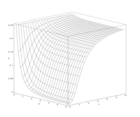
FIG. 1.: Dispersion [Z] of the quadrature component of a pulse at time $t\smash{=}0$ as a function of the maximum nonlinear phase $\psi(0)\smash{=}2\gamma|\alpha^{2}(0)|$ [X] and the reduced frequency $\Omega\smash{=}\omega\tau_{r}$ [Y], at values of the phase of the pulse which are optimal for $\Omega\smash{=}0$.

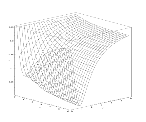
FIG. 2.: Dispersion [Z] of the quadrature component of a pulse at time $t\smash{=}0$ as a function of the maximum nonlinear phase $\psi(0)\smash{=}2\gamma|\alpha^{2}(0)|$ [X] and the reduced frequency $\Omega\smash{=}\omega\tau_{r}$ [Y], at values of the phase of the pulse which are optimal for $\Omega\smash{=}1$.

VI THE WIDTH OF THE SPECTRUM OF SQUEEZED QUADRATURE

From Fig. 1 one can conclude that the frequency where spectral density of ”-quadrature fluctuations” is lower than the shot-noise level, depends on the nonlinear phase addition $\psi_{0}$. Width of the spectrum below the shot-noise level $\Delta\Omega\smash{=}\tau_{r}\Delta\omega$ should be defined from

$$S_{X}(\Delta\Omega,t)=\frac{1}{2}\Bigl{[}\frac{1}{4}+S_{X}(\Omega_{0},t)\Bigl{]}.$$ (114)

Accounting (106,110) for $\Omega_{0}\smash{=}0$ from (114) we have:

$$2\psi(t)\Bigl{[}\psi(t) - \sqrt{1+\psi^{2}(t)}~{}\Bigl{]}L^{2}(\Delta\Omega)+2L(\Delta\Omega)$$ (115)

$$+ \psi(t)\sqrt{1+\psi^{2}(t)}-\psi^{2}(t)-1=0.$$ (116)

Eq.(116) in $L(\Delta\Omega)$ (see (99,100)) has two solution of which only one is real. Solving the (116) for $\Delta\Omega$ we get:

$$\Delta\Omega = \Biggl{[}\frac{2\psi(t)\Bigl{[}\psi(t)-\sqrt{1+\psi^{2}(t)}~{}\Bigl{]}}{-1+\sqrt{1-2\psi(t)\Bigl{[}\psi(t)-\sqrt{1+\psi^{2}(t)}~{}\Bigl{]}}}$$ (118)

$$\times\frac{1}{\sqrt{\Bigl{[}\psi(t)\sqrt{1+\psi^{2}(t)}-\psi^{2}(t)-1\Bigl{]}}}-1\Biggl{]}^{1/2}.$$

From (118) it follows that the change of $\Delta\Omega$ is connected with changes in pulse’s envelope. The frequency band in which the spectral density of the quadrature fluctuations is lower than the shot-noise level depends on the nonlinear phase shift $\psi(t)$. The corresponding dependence at $t\smash{=}0$ for $\omega\smash{=}0$ is displayed in Fig. 3. It may be noted that at $\psi_{0}\smash{\gg}1$ width of the spectrum below the shot noise level is one and a half width of the spectral response of nonlinearity.

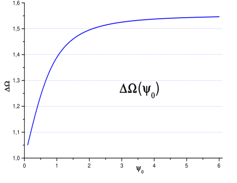
FIG. 3.: Spectral band $\Delta\Omega\smash{=}2\tau_{r}\Delta\omega$ of the quadrature of a pulse with suppressed quantum fluctuations as a function of the maximum nonlinear phase $\psi_{0}$.

VII PHOTON NUMBER SPECTRAL“DENSITY” OF PULSES WITH SELF-PHASE MODULATION

The spectral photon number operator is defined by

$$\hat{n}(\omega,z)=\hat{a}^{+}(\omega,z)\hat{a}(\omega,z),$$ (119)

where:

$$\hat{a}(\omega,z) = \frac{1}{\sqrt{2\pi}\,\tau_{p}}\int_{-\infty}^{\infty}\hat{A}(t,z)e^{i\omega t}dt,$$ (120)

$$\hat{a}^{+}(\omega,z) = \frac{1}{\sqrt{2\pi}\,\tau_{p}}\int_{-\infty}^{\infty}\hat{A}^{+}(t,z)e^{-i\omega t}dt.$$ (121)

Taking into account (120,121) and (25,26) for photon number spectral “density” (119) we find:

$$\bar{n}(\omega,z) = \frac{1}{2\pi\tau^{2}_{p}}\int_{-\infty}^{\infty}\int_{-\infty}^{\infty}\langle\hat{A}^{+}_{0}(t_{1})\,e^{\hat{O}^{+}(t_{1})+\hat{O}(t_{2})}\hat{A}_{0}(t_{2})\rangle$$ (123)

$$\times e^{i\omega(t_{2}-t_{1})}dt_{1}dt_{2}\cong\frac{\bar{n}_{0}}{2\pi}\cdot\frac{1}{\tau^{2}_{p}}\cdot|\mathbf{I}|^{2},$$

where

$${\mathbf{I}}=\int_{-\infty}^{\infty}\rho(t)\,\exp{\left\{i\left[\psi_{0}\rho^{2}(t)+\varphi(t)+\omega t\right]\right\}}dt.$$ (124)

The last expression in (123) is written without the account of $\mu(t_{1},t_{2})$ and $\emph{K}(t_{1},t_{2})$ (see (61)). If the initial pulse has gaussian form $\rho(t)\smash{=}\exp{\{-t^{2}/2\tau^{2}_{p}\}}$ then, using paraxial approximation ($\rho^{2}(t)\cong 1\smash{-}t^{2}/\tau^{2}_{p}$) [11] in (124) for spectral density (123) we find

$$\bar{n}_{class}(\Omega,z)=\frac{\bar{n}_{0}}{\sqrt{1+4\psi^{2}_{0}}}\exp{\left[-\frac{\Omega^{2}}{1+4\psi^{2}_{0}}\right]},$$ (125)

where $\Omega\smash{=}\omega\tau_{p}$. From (125) it follows that the spectral density of a pulse with self-phase modulation (SPM-USP) decreases when nonlinear phase addition increases. To calculate (125) in (123) the terms $\mu(t_{1},t_{2})$ and $K(t_{1},t_{2})$ have not been taken into account. In consequence, the spectral density (125) does not depend on relaxation time. If we take the relaxation function of nonlinearity as [11]

$$\emph{H}(\theta)=\frac{1}{\tau_{r}}\exp{\left\{-\frac{\theta^{2}}{2\tau^{2}_{r}}\right\}}$$ (126)

then $\emph{K}(t,t\smash{+}\tau)=\mu_{0}\rho^{2}(t\smash{+}\tau/2)\exp{\{-\tau^{2}/4\tau^{2}_{r}\}}$. Using the expression $\emph{K}(t,t+\tau)$ in (123) in paraxial approximation we have

$$\bar{n}(\Omega,z)\! = \!\frac{\bar{n}_{0}}{\left[\left(1+\gamma\psi_{0}\nu^{2}/4\right)^{2}+4\psi^{2}_{0}\right]^{1/2}}$$ (128)

$$\times\exp{\left[-\frac{\Omega^{2}\left(1+\gamma\psi_{0}\nu^{2}/4\right)}{\left(1+\gamma\psi_{0}\nu^{2}/4\right)^{2}+4\psi^{2}_{0}}\right]},$$

where $\nu\smash{=}\tau_{p}/\tau_{r}$. From (128) one can conclude that the spectral density depends on the nonlinear phase addition and on the relation between the pulse duration and the relaxation time of the nonlinearity.

VIII THE CORRELATION FUNCTION OF SPECTRAL COMPONENTS OF SPM-USPs

We introduce the correlation function of different spectral components in the following symmetric form:

$$R(\omega_{1},\omega_{2},z)\!\! = \!\!\frac{1}{2}\Bigl{[}\langle\hat{n}(\omega_{1},z)\hat{n}(\omega_{2},z)\rangle\!+\!\langle\hat{n}(\omega_{2},z)\hat{n}(\omega_{1},z)\rangle\!$$ (130)

$$-2\langle\hat{n}(\omega_{1},z)\rangle\langle\hat{n}(\omega_{2},z)\rangle\Bigl{]}.$$

Leaving out the preliminary accounts for (130) we obtain

$$R(\omega_{1},\omega_{2},z)=I_{1}\delta(\omega_{2}\smash{-}\omega_{1})-\frac{1}{2}\psi_{0}Im\{I^{*}_{2}I_{3}+I_{2}I^{*}_{3}\},$$ (131)

$$I_{1}=\int_{-\infty}^{\infty}\int_{-\infty}^{\infty} \widetilde{\rho}(t_{1},t_{2})\exp{\{i[\psi^{2}(t_{1})-\psi^{2}(t_{2})]\}}$$ (134)

$$\times\exp{i[\omega_{1}t_{1}-\omega_{2}t_{2}]}dt_{1}dt_{2},$$

$$I_{2}=\int_{-\infty}^{\infty}\int_{-\infty}^{\infty} \widetilde{\rho}(t_{1},t_{2})\exp{\{i[\psi^{2}(t_{1})+\psi^{2}(t_{2})]\}}$$ (136)

$$\times\exp{\{i[\omega_{1}t_{1}+\omega_{2}t_{2}]\}}dt_{1}dt_{2},$$

$$I_{3}=\int_{-\infty}^{\infty}\int_{-\infty}^{\infty} \widetilde{q}(t_{1},t_{2})\exp{\{i[\psi^{2}(t_{1})+\psi^{2}(t_{2})]\}}$$ (138)

$$\times\exp{\{i[\omega_{1}t_{1}+\omega_{2}t_{2}]\}}dt_{1}dt_{2}.$$

$\widetilde{\rho}(t_{1},t_{2})\smash{=}\rho(t_{1})\rho(t_{2})$, $\widetilde{q}(t_{1},t_{2})\smash{=}\widetilde{\rho}(t_{1},t_{2})\widetilde{h}(t_{2}\smash{-}t_{1})$. If the initial pulse has gaussian form and the relaxation function has the form (126) then in paraxial approximation [11] for correlation function (131) we find

$$R(\Omega_{1},\Omega_{2},z)\!=\!I_{1}\delta(\Omega_{1}\smash{-}\Omega_{2})\smash{-}\frac{\psi_{0}}{2\widetilde{\alpha}\sqrt{\widetilde{\beta}}}Im\{\Gamma(\Omega_{1},\Omega_{2})\},$$ (139)

$$I_{1}=[n_{class}(\Omega_{1})n_{class}(\Omega_{2})]^{1/2}\exp{\Bigl{\{}i\psi_{0}\frac{\Omega^{2}_{1}-\Omega^{2}_{2}}{1+4\psi^{2}_{0}}\Bigl{\}}}.$$ (140)

In (139) are entered the following designations:

$$\Omega=\omega\tau_{p},\qquad\widetilde{\alpha}=\left[1+4\psi^{2}_{0}\right]^{1/2},$$ (141)

$$\widetilde{\beta}=\left[1+2\nu^{2}-4\psi^{2}_{0})^{2}+16(1+\nu^{2})^{2}\psi^{2}_{0}\right]^{1/2},$$ (142)

$${{\Gamma}}(\Omega_{1},\Omega_{2})=\exp{\{G+iS\}}+\exp{\{E+iF\}},$$ (143)

$$Im\Gamma(\Omega_{1},\Omega_{2})=e^{G}\sin{S}+e^{E}\sin{F},$$ (144)

$$G = -\frac{\Omega^{2}_{1}+\Omega^{2}_{2}}{2\widetilde{\alpha}}\cos{\epsilon}-\frac{\Omega^{2}_{2}}{2\varrho}\cos{\Sigma}-\frac{\varrho\,\Omega^{2}_{1}}{2\widetilde{\beta}}\cos{(\Sigma-\xi)}$$ (147)

$$-\frac{\Omega_{1}\Omega_{2}}{\widetilde{\beta}}\nu^{2}\cos{\xi}-\frac{\Omega^{2}_{2}\nu^{4}}{2\varrho\widetilde{\beta}}\cos{(\Sigma+\xi)},$$

$$S = \frac{\Omega^{2}_{1}+\Omega^{2}_{2}}{2\widetilde{\alpha}}\sin{\epsilon}+\frac{\Omega^{2}_{2}}{2\varrho}\sin{\Sigma}-\frac{\varrho\,\Omega^{2}_{1}}{2\widetilde{\beta}}\sin{(\Sigma\smash{-}\xi)}$$ (149)

$$+\frac{\Omega_{1}\Omega_{2}}{\widetilde{\beta}}\nu^{2}\sin{\xi}\smash{+}\frac{\Omega^{2}_{2}\nu^{4}}{2\varrho\widetilde{\beta}}\sin{(\Sigma\smash{+}\xi)}\smash{-}(\epsilon\smash{+}\frac{\xi}{2}),$$

$$E = -\frac{\Omega^{2}_{1}+\Omega^{2}_{2}}{2\widetilde{\alpha}}\cos{\epsilon}-\frac{\Omega^{2}_{1}}{2\varrho}\cos{\Sigma}-\frac{\varrho\,\Omega^{2}_{2}}{2\widetilde{\beta}}\cos{(\Sigma\smash{-}\xi)}$$ (151)

$$-\frac{\Omega_{1}\Omega_{2}}{\widetilde{\beta}}\nu^{2}\cos{\xi}\smash{-}\frac{\Omega^{2}_{1}\nu^{4}}{2\varrho\widetilde{\beta}}\cos{(\Sigma\smash{+}\xi)},$$

$$F = \frac{\Omega^{2}_{1}+\Omega^{2}_{2}}{2\widetilde{\alpha}}\sin{\epsilon}+\frac{\Omega^{2}_{1}}{2\varrho}\sin{\Sigma}-\frac{\varrho\,\Omega^{2}_{2}}{2\widetilde{\beta}}\sin{(\Sigma\smash{-}\xi)}$$ (153)

$$+\frac{\Omega_{1}\Omega_{2}}{\widetilde{\beta}}\nu^{2}\sin{\xi}+\frac{\Omega^{2}_{1}\nu^{4}}{2\varrho\widetilde{\beta}}\sin{(\Sigma\smash{+}\xi)}-(\epsilon\smash{+}\frac{\xi}{2}),$$

$$\varrho = \left[(1+\nu^{2})^{2}+4\psi^{2}_{0}\right]^{1/2},$$ (154)

$$\epsilon = -\arctan{\left\{2\psi_{0}\right\}},$$ (155)

$$\xi = \arctan{\left\{\frac{4(1+\nu^{2})\psi_{0}}{1+2\nu^{2}-4\psi^{2}_{0}}\right\}},$$ (156)

$$\Sigma = \arctan{\left\{\frac{2\psi_{0}}{1+\nu^{2}}\right\}}.$$ (157)

We define the spectral correlation function of the photons with frequency $\Omega$ in the spectral band $\Delta\Omega$

$$\widetilde{R}_{\Delta\Omega}(\Omega,z) = \int_{\Omega-\normalsize{\Delta\Omega/2}}^{\Omega+\normalsize{\Delta\Omega/2}}\int_{\Omega-\normalsize{\Delta\Omega/2}}^{\Omega+\normalsize{\Delta\Omega/2}}R(\Omega_{1},\Omega_{2},z)d\Omega_{1}d\Omega_{2}$$ (159)

$$-\bar{n}_{0}.$$

As a consequence, the conclusion which one can make is that for $\widetilde{R}(\Omega,z)\smash{<}0$ take place the photon antibunching and for $\widetilde{R}(\Omega,z)\smash{>}0$ the photon bunching.

The graphic dependence of the spectral correlation function (159) on $\psi_{0}$ at $\Omega\smash{=}0.04$, $\Delta\Omega\smash{=}2.5\smash{\cdot}10^{-3}$ and $\nu\smash{=}10$ is displayed in Fig.4, whence it follows that the photon bunching or antibunching can take place, and for phases $\psi_{0}\smash{>}1$ it becomes significant.

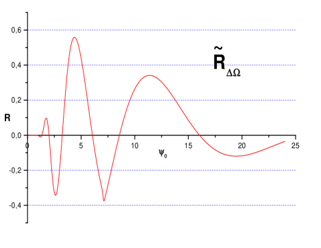
FIG. 4.: Spectral correlation function $\widetilde{R}_{\Delta\Omega}(\Omega,z)$ [R] as a function of the maximum nonlinear phase $\psi_{0}$ measured at the frequency $\Omega\smash{=}0.04$ in spectral band $\Delta\Omega\smash{=}2.5\smash{\cdot}10^{-3}$.

At frequency $\Omega\smash{=}0$, the correlation function (see (159)) has the following simplified form:

$$\widetilde{R}_{\Delta\Omega}(0,z)=\frac{\psi_{0}}{2\widetilde{\alpha}\sqrt{\widetilde{\beta}}}(\Delta\Omega)^{2}\sin{\left(\epsilon\smash{+}\frac{\xi}{2}\right)},$$ (160)

and its dependence on $\psi_{0}$ at $\Delta\Omega\smash{=}0.75$ is shown in Fig. 5, whence it follows that the minimum of the spectral correlation function lies near $\psi_{0}\smash{\approx}1$. In this case the photon antibunching takes place for all phases $\psi_{0}\smash{>}0$ and it is maximal for $\psi_{0}\smash{\approx}1$. It may be mentioned that the greater is the spectral band of measurement the stronger is the photon bunching or antibunching.

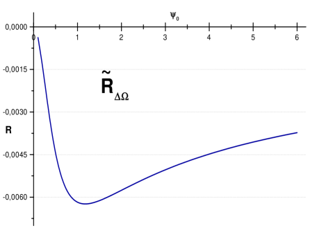
FIG. 5.: Spectral correlation function $\widetilde{R}_{\Delta\Omega}(\Omega,z)$ [R] as a function of the maximum nonlinear phase $\psi_{0}$ measured at the frequency $\Omega=0$ in spectral band $\Delta\Omega=0.75$.

DISCUSSION AND CONCLUSIONS

The results presented in the present paper can be used for the correct interpretation of the results of experiments [2, 3, 12, 13], in which the laser pulses with the duration of the order $100$ ps and quartz optical fibres were used and the maximal meaning of nonlinear phase shift $\psi_{0}$ was greater than $1$. Certainly, in the measurement of the quadrature spectrum the suppression of quantum fluctuations of a pulse will be smoothed out (see (110)). This time over which the “smoothing out” occurs in the case of balanced homodyne detection [14] is determined by the duration of the heterodyne pulse.

The developed theory enables the choice of the optimal strategy at producing and registration of ultrashort pulses in a squeezed states. The measurement of quantum fluctuation of short pulses take place at high frequencies of the order of several tens MHz in order to avoid any effects due to technical fluctuation concentrated at low frequencies. However, in this area the suppression of quantum fluctuations is greatest. The presented results show that by adjusting the phase of the signal pulse (or the phase of a heterodyne pulse), maximal suppression of the quantum fluctuations can be realized at the spectral component of interest for us. This spectral component of interest can lie on the wing of the spectral response of nonlinearity (Fig. 2). This means, that for obtaining squeezed-light pulses the nonlinear media with a longer relaxation time and consequently with the greater nonlinearity can be used [5].

Our results suggest that in the spectral measurements the photon antibunching can be observed. Usually, in the experiments spectral devices with confined spectral bands are used, thus limiting the amplitude of vacuum fluctuations which participate in the measurements. The final results show that the spectral correlation function depends on the nonlinear phase addition, the relation between the pulse duration and the relaxation time of the nonlinearity and also on the spectral band of the measurement. In consequence the choice of the width of the spectral band of measurement can represent an effective method of control of the photon bunching or antibunching. The obtained results indicate that the photon antibunching can be observed at any value of nonlinear phase addition in the low frequency measurements. At high frequency measurements the photon bunching or antibunching strongly depends on the nonlinear phase additions.

We note that the approach developed in the present article can be used to analyse the formation of polarization-squeezed light in media with a cubic nonlinearity. This will be treated in a future publication.

REFERENCES

- [1] M. Kitagava and Y. Yamamoto, Phys. Rev. A, , 3974 (1986).
- [2] N. Nishizawa, M. Hashiura, T. Horio et al, Jpn. J. Appl. Phys., Part 2, , L792 (1998).
- [3] N. Nishizawa, S. Kume, T. Horio et al, Jpn. J. Appl. Phys., Part 1, , 138 (1994).
- [4] M. Shirsaky and H. A. Haus, J. Opt. Soc. Am. B, , 30
- [5] S. A. Akhmanov, V. A. Vysloukh, and A. S. Chirkin, Optics of Femtosecond Laser Pulses, AIP (1992) [Supplemented translation of Russian original, Nauka, Moscow (1988)].
- [6] K. J. Blow, R. Loudon, and S. J. D. Phoenix, J. Opt. Soc. Am. B, 8 1750 (1991).
- [7] L. Boivin, F. X. Kartner, and H. A. Haus, Phys. Rev. Lett. , 240 (1994).
- [8] F. Popescu and A.S. Chirkin, Pis’ma Zh. Eksp. Teor. Fiz, , 481, (1999), [JETP Lett. , 516 (1999)].
- [9] Mooki Toren and Y Ben-Aryeh, Quantum Opt., , 425 (1994).
- [10] K. J. Blow, R. Loudon, S. J. D. Phoenix, T. J. Shepherd, Phys. Rev. A, , 4102 (1990).
- [11] F. Popescu and A.S. Chirkin, Kvant. Elektron. (Moscow), , 61 (1999) [Sov. J. of Quant. Electron. , 61 (1999)].
- [12] M. Rosenblug and R.M. Shelby, Phys. Rev. Lett. , 153 (1991).
- [13] K. Bergman and H. A. Haus, Opt. Lett. , 663 (1991)
- [14] U. Leonhardt, Measuring the Quantum State of Light, Cambridge University Press, 1997.