Robust unravelings for resonance fluorescence

Abstract

Monitoring the fluorescent radiation of an atom unravels the master equation evolution by collapsing the atomic state into a pure state which evolves stochastically. A robust unraveling is one that gives pure states that, on average, are relatively unaffected by the master equation evolution (which applies once the monitoring ceases). The ensemble of pure states arising from the maximally robust unraveling has been suggested to be the most natural way of representing the system [H.M. Wiseman and J.A. Vaccaro, Phys. Lett. A 250, 241 (1998)]. We find that the maximally robust unraveling of a resonantly driven atom requires an adaptive interferometric measurement proposed by Wiseman and Toombes [Phys. Rev. A 60, 2474 (1999)]. The resultant ensemble consists of just two pure states which, in the high driving limit, are close to the eigenstates of the driving Hamiltonian $\Omega\sigma_{x}/2$. This ensemble is the closest thing to a classical limit for a strongly driven atom. We also find that it is possible to reasonably approximate this ensemble using just homodyne detection, an example of a continuous Markovian unraveling. This has implications for other systems, for which it may be necessary in practice to consider only continuous Markovian unravelings.

I Introduction

Some states of open quantum systems are more robust than others. That is, they are less perturbed by the system dynamics. This fact has been the subject of a long-running and active research program [1, 2, 3, 4, 5, 6, 7]. Recently, one of us and Vaccaro have introduced into this program a formalism with a number of distinctive features [8, 9]. This formalism consists of finding the maximally robust unraveling (MRU) for the open quantum system. Its introduction was motivated by a desire to better understand the rich dynamics of open quantum systems in general [8], and that of the atom laser in particular [9].

The use of the term “robust unraveling” rather than “robust state” encapsulates two of the distinctive features of the work of Refs. [8, 9]. An unraveling is a way of measuring the environment of an open quantum system such that the system state can be described by a pure state undergoing stochastic evolution. This is always possible in principle if the unmonitored system obeys a Markovian master equation, which we will assume to have a unique stationary state. In the long time limit, the “unraveled” system will be in a pure state drawn at random from a particular ensemble of pure states defined by the unraveling. It is from the consideration of such an ensemble of pure states that the two distinctive features of our approach are met. The first is that it is not individual pure states whose robustness are to be calculated, but rather a whole ensemble of pure states, the average robustness of which is calculated. The second is that the pure states in this ensemble are physically realizable in the sense that they are the states of the system known to an experimenter using the appropriate measurement scheme on the system’s environment.

As noted above, the principle application of the maximally robust unraveling formalism has been to a model for an atom laser (a continuously damped and replenished gaseous Bose-Einstein condensate). This work is a specialized application in two ways. First, the system itself has a high excitation number and so is a quantum system in the classical limit. Second, only a subset of the set of all possible unravelings was considered. This subset (which is still infinite) contains those unravelings that lead to continuous and Markovian evolution of the system state vector [10]. This restriction was necessary to make the problem tractable and was justified by the classicality of the system.

In this work we apply the formalism of MRU to a system with no classical limit (in the usual sense at least), a resonantly-driven fluorescent two-level atom. This system is one of the canonical examples of an open quantum system, and has surprisingly complex dynamics for its size. It is therefore worth investigating in its own right. But, even more importantly, it is simple enough that the maximally robust unraveling can be found analytically. It turns out that this MRU is neither continuous nor Markovian. This enables us to investigate the question of how closely one can approximate the ensemble of this MRU if one is restricted to considering continuous Markovian unravelings. The answer to this question has implications for the general usefulness of the MRU formalism, since for typical systems it would be necessary to impose this restriction in order to make the formalism practical.

The structure of this paper is as follows. In Sec. II we briefly review the MRU formalism. In Sec. III we introduce the two-level atom model and derive an expression for the ensemble average survival probability (which is used to quantify the robustness) in terms of moments of the ensemble of state vectors. In Sec. IV we look at one simple (but not maximally robust) unraveling, that resulting from direct detection of the atom’s fluorescence, for comparison with other, more robust, unravelings. In Sec. V we present the most robust unraveling and its ensemble of (in this case, just two) state vectors. In Sec. VI we find the most robust unraveling from within the set of continuous Markovian unravelings. We compare this ensemble to the MRU of Sec. V in Sec. VII. We conclude with a discussion of the implications of our results in Sec. VIII.

II Maximally Robust Unravelings

A The Master Equation

Open quantum systems generally become entangled with their environment, and this causes their state to become mixed. In many cases, the system will reach an equilibrium mixed state in the long time limit. This is the sort of system for which our approach to robustness, of finding the maximally robust unraveling (MRU), can be applied without modification.

If the system is weakly coupled to the environmental reservoir, and many modes of the reservoir are roughly equally affected by the system, then one can make the Born and Markov approximations in describing the effect of the environment on the system [11]. Tracing over (that is, ignoring) the state of the environment leads to a Markovian evolution equation for the state matrix $\rho$ of the system, known as a quantum master equation. The most general form of the quantum master equation that is mathematically valid is the Lindblad form [12]

$$\dot{\rho}=-i[H,\rho]+\sum_{\mu=1}^{M}{\cal D}[c_{\mu}]{\rho}\equiv{\cal L}\rho,$$ (1)

where for arbitrary operators $A$ and $B$,

$${\cal D}[A]B\equiv ABA^{\dagger}-(A^{\dagger}AB+BA^{\dagger}A)/2.$$ (2)

If the master equation has a unique stationary state (as we will assume it does), then that is defined by

$${\cal L}\rho_{\rm ss}=0.$$ (3)

This assumption requires that ${\cal L}$ be time-independent. In many quantum optical situations, such as resonance fluorescence, one is only interested in the dynamics in the interaction picture, in which the free evolution at optical frequencies is removed from the state matrix. Indeed, if one treats the driving field as classical, as we will do, it is necessary to move into such an interaction picture in order to obtain a time-independent Liouvillian superoperator ${\cal L}$.

The stationary state matrix $\rho_{\rm ss}$ can be expressed as an ensemble of pure states as follows:

$$\rho_{\rm ss}=\sum_{k}\wp_{k}|{\psi_{k}}\rangle\langle{\psi_{k}}|,$$ (4)

where the $|{\psi_{k}}\rangle$ are normalized state vectors and the $\wp_{k}$ are positive weights summing to unity. The (possibly infinite) set of ordered pairs,

$$E=\{(|{\psi_{k}}\rangle,\wp_{k}):k\},$$ (5)

we will call an ensemble $E$ of pure states. Note that there is no restriction that the states be mutually orthogonal. This means that there are continuously infinitely many ensembles $E$ that represent $\rho_{\rm ss}$. The aim of finding the MRU is to find the “best” or “most natural” representation for $\rho_{\rm ss}$.

B Unravelings

As explained in the Introduction above, the first criterion for our most natural ensemble is that it be physically realizable by monitoring the environment of the system. In the situation where a Markovian master equation can be derived, it is possible (in principle) to continually measure the state of the environment on a time scale large compared to the reservoir correlation time but small compared to the response time of the system. This effectively continuous measurement is what we mean by “monitoring”. In such systems, monitoring the environment does not disrupt the system–reservoir coupling and the system will continue to evolve according to the master equation if one ignores the results of the monitoring.

By contrast, if one does take note of the results of monitoring the environment, then the system will no longer obey the master equation. Because the system–reservoir coupling causes the reservoir to become entangled with the system, measuring the former’s state produces information about the latter’s state. This will tend to undo the increase in the mixedness of the system’s state caused by the coupling.

If one is able to make perfect rank-one projective (i.e. von Neumann) measurements of the reservoir state, the system state will usually be collapsed towards a pure state. However this is not a process that itself can be described by projective measurements on the system, because the system is not being directly measured. Rather, the monitoring of the environment leads to a gradual (on average) decrease in the system’s entropy.

If the system is initially in a pure state then, under perfect monitoring of its environment, it will remain in a pure state. Then the effect of the monitoring is to cause the system to change its pure state in a stochastic and (in general) nonlinear way. Such evolution has been called a quantum trajectory [13], and can be described by a nonlinear stochastic Schrödinger equation for the system state vector [14, 15, 16]. The nonlinearity and stochasticity are present because they are a fundamental part of measurement in quantum mechanics.

On average, the system still obeys the master equation. That is, if the increment in $|{\psi}\rangle$ under the SSE is $|{d\psi}\rangle$ then

$${\rm E}[|{d\psi}\rangle\langle{\psi}|+|{\psi}\rangle\langle{d\psi}|+|{d\psi}\rangle\langle{d\psi}|]={\cal L}{\rm E}[|{\psi}\rangle\langle{\psi}|].$$ (6)

Here ${\rm E}$ denotes the ensemble average with respect to the stochasticity of the SSE. This stochasticity is evidenced by the necessity of retaining the Itô term $|{d\psi}\rangle\langle{d\psi}|$ [17].

Because the ensemble average of the system still obeys the master equation, the stochastic Schrödinger equation) is said to unravel the master equation [13]. It is now well-known that there are many (in fact continuously many) different unravelings for a given master equation [18], corresponding to different ways of monitoring the environment.

Each unraveling ${\cal U}$ gives rise to an ensemble of pure states

$$E^{\cal U}=\{(|{\psi_{k}^{\cal U}}\rangle,\wp_{k}^{\cal U}):k\},$$ (7)

where $|{\psi_{k}^{\cal U}}\rangle$ are the possible pure states of the system at steady state, and $\wp_{k}^{\cal U}$ are their weights. For master equations with a unique stationary state $\rho_{\rm ss}$, the SSE is ergodic over $E^{\cal U}$ [19] and $\wp_{k}^{\cal U}$ is equal to the proportion of time the system spends in state $|{\psi_{k}^{\cal U}}\rangle$. The ensemble $E^{\cal U}$ represents $\rho_{\rm ss}$ in that

$$\sum_{k}\wp_{k}^{\cal U}|{\psi_{k}^{\cal U}}\rangle\langle{\psi_{k}^{\cal U}}|=\rho_{\rm ss},$$ (8)

as guaranteed by Eq. (6).

C Survival Probability

Imagine that the system has been evolving under a particular unraveling ${\cal U}$ from an initial state at time $-\infty$ to the stationary ensemble at the present time $0$. It will then be in the state $|{\psi_{k}^{\cal U}}\rangle$ with probability $\wp_{k}^{\cal U}$. If we now cease to monitor the system then the state will no longer remain pure, but rather will relax toward $\rho_{\rm ss}$ under the evolution of Eq. (1).

This relaxation to equilibrium will occur at different rates for different states. For example, some unravelings will tend to collapse the system into a pure state that is very fragile, in that it changes into a very different (and mixed) state as it relaxes to equilibrium. In this case the ensemble would rapidly become a poor representation of the observer’s expected knowledge about the system. Hence we can say that such an ensemble is a “bad” or “unnatural” representation of $\rho$. Conversely, an unraveling that produces robust states would remain an accurate description for a relatively long time. We expect such a “good” or “natural” ensemble to give more intuition about the dynamics of the system. The most robust ensemble we interpret as the “best” or “most natural” such ensemble.

We quantify the robustness of a particular state $|{\psi_{k}^{\cal U}}\rangle$ by its survival probability $S_{k}^{\cal U}(t)$. This is the probability that the system would be found (by a hypothetical projective measurement) to still be in the state $|{\psi_{k}^{\cal U}}\rangle$ at time $t$. It is given by

$$S_{k}^{\cal U}(t)=\langle{\psi_{k}^{\cal U}}|e^{{\cal L}t}\left[{|{\psi_{k}^{\cal U}}\rangle\langle{\psi_{k}^{\cal U}}|}\right]|{\psi_{k}^{\cal U}}\rangle.$$ (9)

Since we are considering an ensemble $E^{\cal U}$ we must define the average survival probability

$$S^{\cal U}(t)=\sum_{k}\wp_{k}^{\cal U}S_{k}^{\cal U}(t).$$ (10)

In the limit $t\to\infty$ the ensemble-averaged survival probability will tend towards the stationary value

$$S^{\cal U}(\infty)={\rm Tr}[\rho_{\rm ss}^{2}].$$ (11)

This is independent of the unraveling ${\cal U}$ and is a measure of the mixedness of $\rho_{\rm ss}$.

There are many possible figures-of-merit that may be obtained from the survival probability $S^{\cal U}(t)$, as discussed in Ref. [9]. Here we choose the simplest one, also adopted in [9]: the time it takes for $S^{\cal U}(t)$ to fall half-way to its equilibrium value. That is,

$$\tau^{\cal U}={\rm min}\{t\,:\,S^{\cal U}(t)=(1+{\rm Tr}[\rho_{\rm ss}^{2}])/2\}.$$ (12)

This survival time $\tau^{\cal U}$ quantifies the robustness of a particular unraveling ${\cal U}$.

Let the set of all unravelings be denoted $J$. Then the subset of maximally robust unravelings $J_{M}$ is

$$J_{M}=\{{\cal R}\in J:\tau^{\cal R}\geq\tau^{\cal U}\;\forall\,{\cal U}\in J\}.$$ (13)

Even if $J_{M}$ has many elements ${\cal R}_{1},{\cal R}_{2},\ldots$, these different unravelings may give the same ensemble $E^{\cal R}=E^{{\cal R}_{1}}=E^{{\cal R}_{2}}=\ldots$. In this case we claim $E^{\cal R}$ is the most natural ensemble representation of the stationary solution of a given master equation. Different definitions of survival time [8, 9] will obviously lead to different numerical values for $\tau^{\cal R}$. We are less concerned with such numerical values than with the robust ensemble $E^{\cal R}$, which has been found [9] to depend little on the precise definition used.

III The Two-Level Atom

A The Resonance Fluorescence Master Equation

Consider an atom with two relevant levels $\{|{g}\rangle,|{e}\rangle\}$. Let there be a dipole moment between these levels so that the coupling to the continuum of electromagnetic field modes in the vacuum state will cause the atom to decay at rate $\gamma$. So that the atom does not simply decay to the state $|{g}\rangle$, add driving by a classical field (such as that produced by a laser) of Rabi frequency $\Omega$. We work in the interaction picture with respect to the free Hamiltonian $H_{0}=\hbar\omega_{0}|{e}\rangle\langle{e}|$ so that the classical driving at frequency $\omega$ becomes time-independent. The evolution of the atom’s state matrix can then be described by the resonance fluorescence (RF) master equation

$$\dot{\rho}=-i\frac{\Omega}{2}[\sigma_{x},\rho]+\gamma{\cal D}[\sigma]\rho.$$ (14)

In this equation we have used the Pauli matrices

$$\sigma_{x} = |e\rangle\langle g|+|g\rangle\langle e|$$ (15)

$$\sigma_{y} = -i|e\rangle\langle g|+i|g\rangle\langle e|$$ (16)

$$\sigma_{z} = |e\rangle\langle e|-|g\rangle\langle g|$$ (17)

$$\sigma = |g\rangle\langle e|=\frac{1}{2}(\sigma_{x}-i\sigma_{y})$$ (18)

$$\sigma^{\dagger} = |e\rangle\langle g|=\frac{1}{2}(\sigma_{x}+i\sigma_{y})$$ (19)

In terms of these, any state of the atom can be written as a 3-vector $(x,y,z)$ satisfying

$$x^{2}+y^{2}+z^{2}\leq 1,$$ (20)

with equality only for a pure state. From this Bloch vector the state matrix is defined by

$$\rho=\frac{1}{2}\left(I+x\sigma_{x}+y\sigma_{y}+z\sigma_{z}\right).$$ (21)

The linear equations of motion for the Bloch vector that result from Eq. (14) are known as the Bloch equations. The solution satisfying the initial condition

$$x(0)=u\;\;,\;y(0)=v\;\;,\;z(0)=w$$ (22)

is

$$x(t) = ue^{-(\gamma/2)t},$$ (23)

$$y(t) = c_{+}e^{\lambda_{+}t}+c_{-}e^{\lambda_{-}t}+y_{\rm ss},$$ (24)

$$z(t) = c_{+}\frac{\gamma-4i\tilde{\Omega}}{4\Omega}e^{\lambda_{+}t}+c_{-}\frac{\gamma+4i\tilde{\Omega}}{4\Omega}e^{\lambda_{-}t}+z_{\rm ss}.$$ (25)

Here $c_{\pm}$ are constants given by

$$c_{\pm}=\frac{1}{8i\tilde{\Omega}}\left[\mp 4\Omega(w-z_{\rm ss})\pm(\gamma\pm 4i\tilde{\Omega})(v-y_{\rm ss})\right].$$ (26)

The eigenvalues $\lambda_{\pm}$ are defined by

$$\lambda_{\pm}=-\frac{3}{4}\gamma\pm i\tilde{\Omega}.$$ (27)

Here

$$\tilde{\Omega}=\sqrt{\Omega^{2}-({\gamma}/{4})^{2}}$$ (28)

is a real modified Rabi frequency for $\Omega>\gamma/4$, and is imaginary for $\Omega<\gamma/4$. The stationary solutions appearing in the above equations are

$$x_{\rm ss} = 0,$$ (29)

$$y_{\rm ss} = \frac{2\gamma\Omega}{\gamma^{2}+2\Omega^{2}},$$ (30)

$$z_{\rm ss} = \frac{-\gamma^{2}}{\gamma^{2}+2\Omega^{2}}.$$ (31)

B The Survival Probability

Using the Bloch vector representation of the atomic state matrix it is easy to show that the survival probability for a pure state $|{\psi_{k}}\rangle$ with projector

$$|{\psi_{k}}\rangle\langle{\psi_{k}}|=\frac{1}{2}\left({1+u_{k}\sigma_{x}+v_{k}\sigma_{y}+w_{k}\sigma_{z}}\right)$$ (32)

is

$$S_{k}(t)=\frac{1}{2}\left({1+x_{k}(t)u_{k}+y_{k}(t)v_{k}+z_{k}(t)w_{k}}\right),$$ (33)

where $(x,y,z)_{k}(t)$ is the Bloch vector at time $t$ with the initial condition $(x,y,z)_{k}(0)=(u,v,w)_{k}$ as in Eqs. (23)–(25). From that solution it is evident that $S_{k}(t)$ will contain terms that are constant, linear, and bilinear in the vector components $(u,v,w)_{k}$ of the initial state.

As explained in the preceding section we are interested in the survival probability not for a single state but for an ensemble of states. This is the ensemble average of Eq. (10). After some work, the survival probability in this case is found to be simply

$$S(t) = \sum_{k}\wp_{k}S_{k}(t)$$ (34)

$$= \frac{1}{2}(1+y_{\rm ss}^{2}+z_{\rm ss}^{2})+\frac{1}{2}$$ (36)

$$\times\;\left[{(1-y_{\rm ss}^{2}-z_{\rm ss}^{2})e^{-(\gamma/2)t}+V_{v}f_{+}(t)+V_{w}f_{-}(t)}\right],$$

where

$$f_{\pm}(t)=-e^{-(\gamma/2)t}+e^{-(3\gamma/4)t}\left({\cos\tilde{\Omega}t\pm\frac{\gamma}{4\tilde{\Omega}}\sin\tilde{\Omega}t}\right).$$ (37)

In Eq. (36), all the information about the ensemble is contained in the moments

$$V_{v} \equiv {\rm E}[v^{2}]-E[v]^{2}=\sum_{k}\wp_{k}v_{k}^{2}-\left({\sum_{k}\wp_{k}v_{k}}\right)^{2},$$ (38)

$$V_{w} \equiv {\rm E}[w^{2}]-E[w]^{2}=\sum_{k}\wp_{k}w_{k}^{2}-\left({\sum_{k}\wp_{k}w_{k}}\right)^{2}.$$ (39)

This is possible because we have used the following relations:

$${\rm E}[(u,v,w)] = (x_{\rm ss},y_{\rm ss},z_{\rm ss}),$$ (40)

$${\rm E}[u^{2}] = 1-{\rm E}[v^{2}]-{\rm E}[w^{2}].$$ (41)

To find the robustness of any particular unraveling we thus need to find simply the two ensemble averages $V_{v}$ and $V_{w}$.

IV Unraveling by Direct Detection

The most obvious way to unravel the RF master equation is by direct detection. This requires detecting all of the atom’s fluorescence by unit-efficiency photodetectors. This is beyond current technology, but not by so much that the experiment should be considered unphysical. As we will find, unraveling by direct detection is actually not very robust (by the definition of Sec. II) but it is nevertheless useful to consider as a point of comparison with more robust unravelings.

The stochastic evolution of an atom undergoing RF with direct detection has been considered many times before [13, 16]. It has one feature that enables an enormous simplification over a generic unraveling. This is that immediately following a detection, the atomic state is independent of its state before, and is just the ground state $|{g}\rangle$. Between these jumps to the ground state, the conditioned atomic state evolves deterministically. At steady state, when there has certainly been at least one detection, all members of the ensemble are therefore identified simply by the time $t$ since the last detection.

If there is a detection at time $t_{0}$, then, until the next detection occurs, the state of the atom at time $t_{0}+t$ evolves according to the equation [13, 16]

$$\frac{d}{dt}|\tilde{\psi}_{0}(t)\rangle=-\left(\frac{\gamma}{2}\sigma^{\dagger}\sigma-i\frac{\Omega}{2}\sigma_{x}\right)|\tilde{\psi}_{0}(t)\rangle.$$ (42)

The solution, satisfying the initial condition $|{\tilde{\psi}_{0}(0)}\rangle=|{g}\rangle$ is

$$|\tilde{\psi}_{0}\rangle=\tilde{c}_{e}(t)|e\rangle+\tilde{c}_{g}(t)|g\rangle,$$ (43)

where

$$\tilde{c}_{g}(t) = \left[{\cos(\check{\Omega}t/2)+\frac{\gamma}{2\check{\Omega}}\sin(\check{\Omega}t/2)}\right]e^{-(\gamma/4)t},$$ (44)

$$\tilde{c}_{e}(t) = -i\frac{\Omega}{\check{\Omega}}\sin(\check{\Omega}t/2)e^{-(\gamma/4)t}.$$ (45)

Here

$$\check{\Omega}=\sqrt{\Omega^{2}-(\gamma/2)^{2}}$$ (46)

is a real modified Rabi frequency for $\Omega>\gamma/2$ and is imaginary for $\Omega<\gamma/2$. Note that it is different from $\tilde{\Omega}$ defined in Eq. (28).

The state in Eq. (43) is unnormalized, and the norm $\langle{\tilde{\psi}_{0}(t)}|{\tilde{\psi}_{0}(t)}\rangle$ represents the probability that there has been no detection since time $t_{0}$, given that there was a detection at that time. Let us write this probability as

$$P_{0}(t)=|\tilde{c}_{e}(t)|^{2}+|\tilde{c}_{g}(t)|^{2}.$$ (47)

We show in the appendix that this probability is related to $\wp(t)$, the probability that, at steady state, the last detection was a time $t$ ago, by

$$\wp(t)=\frac{P_{0}(t)}{\int_{0}^{\infty}P_{0}(s)ds}.$$ (48)

As noted above, in steady state under direct detection the possible atomic states are parametrized by the real variable $t$, the time since the last detection. The state at that time has projector

$$\hat{P}(t)=\frac{|{\tilde{\psi}_{0}(t)}\rangle\langle{\tilde{\psi}_{0}(t)}|}{\langle{\tilde{\psi}_{0}(t)}|{\tilde{\psi}_{0}(t)}\rangle},$$ (49)

and the weight for each of these members of the ensemble is $\wp(t)dt$. Physically, all members of the ensemble exist on the $u=0$ great circle of the Bloch sphere, because that is where the modified Rabi cycling of Eq. (42) takes the ground state. This distribution is shown in Fig. 1(a). For $\check{\Omega}$ imaginary (that is, $\Omega<\gamma/2$) the states never reach the excited state. For $\check{\Omega}$ real (that is, $\Omega>\gamma/2$, the states may undergo an arbitrary number of cycles. For $\Omega\gg\gamma$ the states are likely to undergo many cycles before a spontaneous emission event occurs so that the ensemble consists of all the states on the $u=0$ great circle, almost uniformly distributed.

From Eq. (49) it can be verified analytically that

$$\int_{0}^{\infty}\hat{P}(t)\wp(t)dt=\frac{1}{\cal N}\int_{0}^{\infty}dt|{\tilde{\psi}_{0}(t)}\rangle\langle{\tilde{\psi}_{0}(t)}|=\rho_{\rm ss},$$ (50)

where

$${\cal N}=\int_{0}^{\infty}\left[{|\tilde{c}_{e}(t)|^{2}+|\tilde{c}_{g}(t)|^{2}}\right]dt.$$ (51)

. Moreover we can easily find numerically the ensemble averages necessary to find the ensemble average survival probability, namely

$$V_{v} = \frac{1}{\cal N}\int_{0}^{\infty}\frac{[i\tilde{c}_{e}(t)\tilde{c}_{g}^{*}(t)-i\tilde{c}_{e}^{*}(t)\tilde{c}_{g}(t)]^{2}}{|\tilde{c}_{e}(t)|^{2}+|\tilde{c}_{g}(t)|^{2}}dt-y_{\rm ss}^{2},$$ (52)

$$V_{w} = \frac{1}{\cal N}\int_{0}^{\infty}\frac{[|\tilde{c}_{e}(t)|^{2}-|\tilde{c}_{g}(t)|^{2}]^{2}}{|\tilde{c}_{e}(t)|^{2}+|\tilde{c}_{g}(t)|^{2}}dt-z_{\rm ss}^{2},$$ (53)

In Fig. 2 we plot the survival probability for the direct detection ensemble, for a variety of driving strengths $\Omega$. We see that for $\Omega<\gamma$ the survival probability decays approximately exponentially at rate of order $\gamma$. For $\Omega\ll\gamma$ the stationary state matrix is close to the ground state, and most members of the direct detection ensemble are also. For $\Omega\gg\gamma$ the ensemble is equally spread over the $u=0$ great circle and consequently the variances $V_{v}$ and $V_{w}$ are approximately equal to $1/2$. Using this, the survival probability is found to be approximately

$$S(t)\approx\frac{1}{2}\left({1+e^{-(3/4)\gamma t}\cos\tilde{\Omega}t}\right).$$ (54)

The oscillations in the survival probability are due to the Rabi oscillations. As noted above, the direct detection ensemble consists of states on the $u=0$ great circle. Rabi cycling around the $x$-axis according to the RF master equation (14) rotates this circle around, rapidly moving the states away from their initial positions and then back close to their initial conditions after one cycle. They do not return exactly to their initial states because of the slow (at rate $3\gamma/4$) decay towards the equilibrium state. This behaviour is illustrated for a typical member of the direct detection ensemble in Fig. 1(b).

The change from damped to oscillatory behaviour has a dramatic effect on the survival time in Eq. (12). It is plotted in Fig. 3 as a function of $\Omega$. For $\Omega\ll\gamma$ it is given by

$$\tau\simeq 2\ln 2\gamma^{-1},$$ (55)

as in this limit the survival probability decays as $e^{-\gamma t/2}$. For $\Omega\gg\gamma$, we can use Eq. (54) to get the approximate expression

$$\tau\simeq\frac{\pi}{3}\Omega^{-1}.$$ (56)

That is, the survival time is here determined by the Hamiltonian evolution only. As shown in Fig. 3, this is quite a good approximation even for moderate $\Omega$.

V The Most Robust Unraveling

A The Most Robust Ensemble

It was stated above that the unraveling by direct detection is not the most robust unraveling. In fact, from an examination of the survival probability in Eq. (36) we can see that it is one of the least robust unravelings for $\Omega\gg\gamma$. That is because of the large variances in $v$ and $w$ in this limit.

It is not difficult to show that the two functions $f_{+}(t)$ and $f_{-}(t)$, defined in Eq. (37), are non-positive for all $\Omega$ and for $t>0$. Since the variances $V_{v}$ and $V_{w}$ are non-negative, it is easy to see that to maximize the survival probability, one would wish to minimize $V_{v}$ and $V_{w}$. The ideal limit would be $V_{v}=V_{w}=0$. This corresponds to an ensemble in which all members have the same Bloch vector components $v$ and $w$. Since the ensemble average must equal $\rho_{\rm ss}$ it follows then that for all members

$$v=y_{\rm ss}\;,\;\;w=z_{\rm ss}.$$ (57)

Furthermore, since $x_{\rm ss}=0$, and since the members of the ensemble must be pure, it follows that for all members

$$u=\pm\sqrt{1-y_{\rm ss}^{2}-z_{\rm ss}^{2}},$$ (58)

where the two alternatives are equally weighted. These two members of the ensemble are shown in Fig. 1(c).

This ensemble is guaranteed to give the maximum survival probability

$$S(t)=\frac{1}{2}(1+y_{\rm ss}^{2}+z_{\rm ss}^{2})+\frac{1}{2}\left[{(1-y_{\rm ss}^{2}-z_{\rm ss}^{2})e^{-(\gamma/2)t}}\right],$$ (59)

which is plotted in Fig. 5. It gives the maximum survival time

$$\tau=2\ln 2\gamma^{-1},$$ (60)

which is independent of $\Omega$. There is no Rabi cycling because the states defined by the Bloch vector $(u,v,w)$ have $v$ and $w$ already equal to their stationary values. Under the master equation evolution $u$ simply decays towards its stationary value of zero and $v$ and $w$ remain constant. This decay of the Bloch vector to equilibrium at rate $\gamma/2$ is shown in Fig. 1(d).

B Adaptive Interferometric Detection

The most robust ensemble defined here would be a mere curiosity if it were not for the fact that there is a detection scheme that realizes it. This scheme, proposed by one of us and Toombes [20], involves interfering the light from the atom with a resonant local oscillator before detection. This is done using a highly transmitting beam splitter as shown in Fig. 4. In the limit of a large local oscillator, this is known as homodyne detection. However we require a very weak local oscillator, with reflected intensity comparable to the intensity of the light from the atom. Furthermore, we require the local oscillator amplitude to be continually adjusted by a real-time feedback loop. To be specific, the field detected should be proportional to

$$\sigma+\mu(t),$$ (61)

where the field from the atom is proportional to $\sigma$, the atomic lowering operator as usual, and the local oscillator field is represented by the complex number $\mu(t)$. This complex number is given by

$$\mu(t)=\pm\frac{1}{2},$$ (62)

where the sign is changed every time a detection occurs.

Remarkably, this relatively simple detection scheme has the consequence that, after initial transients have died away, a driven atom jumps between the states with projector $\hat{P}_{\pm}$, where

$$\hat{P}_{\pm}=\frac{1}{2}\left({I\pm\sqrt{1-y_{\rm ss}^{2}-z_{\rm ss}^{2}}\sigma_{x}+v_{\rm ss}\sigma_{y}+w_{\rm ss}\sigma_{z}}\right),$$ (63)

every time a detection occurs. The rate of detections moreover is independent of which of these states the atom is in, and is equal to $\gamma/4$. Thus in the long time limit the atom will have a probability $\wp_{\pm}=1/2$ to be in each of them, and the maximally robust ensemble will be physically realized.

VI Continuous Markovian Unravelings

The most robust unraveling is neither continuous nor Markovian. It is not continuous because the atomic state jumps every time there is a detection. It is not Markovian because the evolution of the atomic state does not depend only on its present state. Rather, it depends on the past history of detections through the local oscillator amplitude $\mu(t)$. As noted in the introduction, previous investigations of robust unravelings in other systems[8, 9] have been restricted to unravelings that do have these properties. It is therefore interesting to ask for the present system, how close to the MRU is the most robust unraveling that is continuous and Markovian?

Continuous Markovian unraveling (CMU) of the RF master equation (14) can be represented by a two-parameter family of nonlinear SSEs for the non-normalized state vector $|{\bar{\psi}(t)}\rangle$ of the form

$$d|{\bar{\psi}(t)}\rangle=dt\left[{-iH-\frac{\gamma}{2}\sigma^{\dagger}\sigma+J(t)\sigma}\right]|{\bar{\psi}(t)}\rangle,$$ (64)

which is to be interpreted in the Itô sense [17]. Here $J(t)$ is a complex “current” given by

$$J(t)dt=\gamma\left\langle{\upsilon\sigma+\sigma^{\dagger}}\right\rangle dt+\sqrt{\gamma}\,dW(t),$$ (65)

where $\upsilon$ is a complex number satisfying

$$\upsilon^{*}\upsilon\leq 1,$$ (66)

and the angle brackets denote a quantum average using the normalized state vector $|{\psi(t)}\rangle$. We use $|{\bar{\psi}}\rangle$ rather than $|{\tilde{\psi}}\rangle$ because the norm of $|{\bar{\psi}}\rangle$ has no interpretation in terms of probability, unlike that of $|{\tilde{\psi}}\rangle$ in Sec. IV. The stochastic term $dW(t)$ is a complex Gaussian white noise term satisfying

$${\rm E}[dW] = 0,$$ (67)

$${\rm E}[dW^{*}dW] = dt,$$ (68)

$${\rm E}[(dW)^{2}] = \upsilon dt.$$ (69)

The complex parameter $\upsilon$ comprises the two parameters for the family of unravelings of the form of Eq. (64). From Eq. (67) and Eq. (68) it can be shown that Eq. (6) is satisfied for all $\upsilon$. Thus

$$\rho(t)={\rm E}\left[{\frac{|{\bar{\psi}(t)}\rangle\langle{\bar{\psi}(t)}|}{\langle{\bar{\psi}(t)}|{\bar{\psi}(t)}\rangle}}\right]$$ (70)

obeys the RF master equation (14), while in an individual trajectory the state remains pure. In this case there is no simple way to find the steady state ensemble of pure states. A numerical simulation of Eq. (64), with time averages replacing ensemble averages, is the only way to proceed.

Finding the maximally robust continuous Markovian unraveling (MRCMU) in this case reduces to a search over the ball $|\upsilon|^{2}\leq 1$ in the complex plane. We find that the MRCMU is for $\upsilon=1$. For this value of $\upsilon$ the “current” $J(t)$ (which is real in this case) has a deterministic part equal to

$${\rm E}\left[{J(t)}\right]=\gamma\left\langle{\sigma_{x}}\right\rangle.$$ (71)

That is, the measurement yields information about the $\sigma_{x}$ quadrature of the atomic dipole. As a consequence it tends to localize the atom near the $\sigma_{x}$ eigenstates. This localization is relatively stable for high driving, since these are also eigenstates of the Hamiltonian $\Omega\sigma_{x}/2$. This is shown in Fig. 1(e), which is a stochastically generated sample of 10000 states from the equilibrium ensemble for the MRCMU. In complete contrast to the direct detection ensemble in Fig. 1(a), most of the states lie close to the $\sigma_{x}$ eigenstates. For $\Omega$ large as in this figure, this means close to the two members of the MRU shown in Fig. 1(c).

Because a typical member of the MRCMU ensemble is fairly close to the $\sigma_{x}$ axis, it is relatively little affected by the Hamiltonian, which causes rotation around that axis. Under the RF master equation (14) its evolution consists of decay to the equilibrium, with relatively small Rabi oscillations superimposed. This is as shown in Fig. 1(f). As a consequence, although the survival probability oscillates, it remains above its equilibrium value and decays towards it at a rate proportional to $\gamma$. This is shown in Fig. 5 for $\Omega=10\gamma$. Also shown, for comparison, is the survival probability for the minimally robust CMU, which occurs for $\upsilon=-1$. This is almost identical to the corresponding curve for direct detection in Fig. 2, as the ensemble is confined to the $u=0$ great circle in both cases.

The survival time for the MRCMU is shown in Fig. 3. Because of our definition of survival time in Eq. (12), the survival time for the MRCMU is determined by the rapid (for $\Omega\gg\gamma$) oscillations in the survival probability rather than the slow mean decay. Thus it is qualitatively similar to the survival time for the direct detection ensemble, starting at $2\ln 2\gamma^{-1}$ and then falling like $\Omega^{-1}$ as $\Omega$ increases.

VII Comparison of the MRU and the MRCMU

We have seen that no continuous Markovian unraveling (CMU) is as robust as the maximally robust unraveling (MRU), which is neither continuous nor Markovian. Furthermore, the robustness for the maximally robust CMU, as measured by the survival time, scales in the same way as that for the very non-robust direct detection scheme. However, because of the arbitrariness in any definition of survival time, we are interested more in the robust ensembles themselves than in the numerical values of their survival times. As discussed above, the MRCMU realizes an ensemble that has a common feature with that realized by the MRU: the states in the ensemble tend to have well-defined values of $u=\left\langle{\sigma_{x}}\right\rangle$. In this section we wish to answer the question: just how close is the MRCMU ensemble to the MRU ensemble?

A Closeness of Two Ensembles

To answer this question we require a measure (not necessarily transitive) from ensemble $E^{A}$ to ensemble $E^{B}$, where each ensemble represents the same state matrix. It seems best to choose an operationally defined measure, which we do as follows.

By allowing the same projector to reappear with different indices, we can write, to any desired degree of accuracy,

$$E^{A} = \left\{{(|{\phi_{k}}\rangle,N^{-1}):1\leq k\leq N}\right\},$$ (72)

$$E^{B} = \left\{{(|{\psi_{\mu}}\rangle,N^{-1}):1\leq\mu\leq N}\right\},$$ (73)

where $|{\phi_{k}}\rangle$ and $|{\psi_{\mu}}\rangle$ are normalized states such that

$$\rho=N^{-1}\sum_{k}|{\phi_{k}}\rangle\langle{\phi_{k}}|=N^{-1}\sum_{\mu}|{\psi_{\mu}}\rangle\langle{\psi_{\mu}}|,$$ (74)

where $N$ is an arbitrarily large integer.

To define the closeness of the ensembles, imagine that there are two people, Alice and Bob. Alice has in her possession a measuring device with $N$ settings, corresponding to the $N$ projectors $\{|{\phi_{k}}\rangle\langle{\phi_{k}}|:k\}$. If setting $k$ is chosen then the device makes a projective measurement with projector $|{\phi_{k}}\rangle\langle{\phi_{k}}|$. Bob has in his possession an ensemble of quantum states $\{|{\psi_{\mu}}\rangle:\mu\}$. It is Bob’s aim to try to convince Alice that he is actually in possession of the ensemble $\{|{\phi_{k}}\rangle:k\}$. He must submit each of his $N$ systems $|{\psi_{\mu}}\rangle$ to Alice, telling her which of her states $|{\phi_{k}}\rangle$ each is supposed to be in. She then makes the appropriate measurement and, unless Bob’s ensemble really is the same as Alice’s, is likely to find errors some of the time. An error is when a state that Bob claims is $|{\psi_{k}}\rangle$ is found to give the answer “no” to Alice’s projective measurement “is the state $|{\phi_{k}}\rangle$?” Assuming Bob chooses a good strategy, then the higher the probability of error, the larger the distance between the two ensembles.

We can formalize this as follows. Say Bob actually sends state $|{\psi_{\mu}}\rangle$, but claims it is $|{\phi_{k(\mu)}}\rangle$, where the functional dependence here indicates that Bob makes his choice of index $k$ based on his actual state. Then the probability of error for this state is

$$\epsilon_{k(\mu)|\mu}=1-\left|\langle{\phi_{k(\mu)}}|{\psi_{\mu}}\rangle\right|^{2}.$$ (75)

The ensemble average probability of error, for Bob’s optimum strategy, is

$$\epsilon_{\rm opt}=N^{-1}\min_{M}\sum_{\mu=1}^{N}\epsilon_{k(\mu)|\mu},$$ (76)

where the minimum is over all one-to-one mappings $M$

$$\mu\stackrel{{\scriptstyle M}}{{\longrightarrow}}k(\mu)\;,\;\;k\stackrel{{\scriptstyle M^{-1}}}{{\longrightarrow}}\mu(k).$$ (77)

Bob’s strategies have to correspond to a mapping of this form because unless Bob names each of Alice’s states once and once only Alice would know that Bob is lying when he claims to be in possession of Alice’s ensemble $\{|{\phi_{k}}\rangle:k\}$.

We could take the distance between the ensembles to be equal to this minimum average error probability. However, if the state matrix $\rho$ is close to being pure (with ${\rm Tr}[\rho^{2}]$ close to one), then the average error probability would be small regardless of what strategy Bob chose. In particular, if Bob had a totally random strategy then the error probability for an individual state $|{\psi_{\mu}}\rangle$ would be, on average,

$$\langle\epsilon_{k|\mu}\rangle=1-\langle{\psi_{\mu}}|\overline{|{\phi_{k}}\rangle\langle{\phi_{k}}|}|{\psi_{\mu}}\rangle=1-\langle{\psi_{\mu}}|\rho|{\psi_{\mu}}\rangle,$$ (78)

and the ensemble average error probability would be

$$\overline{\epsilon}=N^{-1}\sum_{\mu=1}^{N}\left({1-{\rm Tr}[\rho|{\psi_{\mu}}\rangle\langle{\psi_{\mu}}|]}\right)=1-{\rm Tr}[\rho^{2}].$$ (79)

That is, the average error probability would be close to zero even though Bob does not take into account the difference between his states so that his effective ensemble consists of $N$ copies of the mixed state $\rho$.

For this reason, it seems better to define the distance between the ensembles by the normalized error probability:

$$d(E^{A}|E^{B})=\frac{1-\min_{M}\sum_{\mu=1}^{N}\frac{1}{N}\left|\langle{\phi_{k(\mu)}}|{\psi_{\mu}}\rangle\right|^{2}}{1-{\rm Tr}[\rho^{2}]}.$$ (80)

In this case it is easy (at least for a two-level system) to see that

$$0\leq d(E^{B}|E^{A})\leq 1,$$ (81)

where the lower bound is attained if and only if the ensembles are identical, and where no tighter upper bound can be found for a given $\rho$. Thus the two ensembles could be said to be close if and only if $d(E^{B}|E^{A})\ll 1$.

B Closeness of the MRU and MRCMU Ensembles

In the case at hand the reference ensemble $E^{A}$ is the most robust ensemble of Sec. V, while the ensemble $E^{B}$ whose closeness we wish to gauge is that of the most robust continuous Markovian unraveling of Sec. VI. The fact that $E^{A}$ has only two elements, whereas $E^{B}$ has an infinitude of elements causes no problems. We simply allow an arbitrarily large number $N$ of elements for each ensemble and let half of those for ensemble $A$ be the state with projector $\hat{P}_{+}$ and half the state $\hat{P}_{-}$, as defined in Eq. (63).

Because the two states $\hat{P}_{\pm}$ differ only by the sign of $\left\langle{\sigma_{x}}\right\rangle$, and because both ensembles are symmetric about a reflection in the $y-z$ plane, Bob’s best strategy is easy to find. For each of his states $|{\psi_{\mu}}\rangle$ he tells Alice that it is state $\hat{P}_{+}$ if it has a positive mean $\sigma_{x}$, and $\hat{P}_{-}$ if it has a negative mean $\sigma_{x}$. If $|{\psi_{\mu}}\rangle$ is the state

$$|{\psi_{\mu}}\rangle\langle{\psi_{\mu}}|=\frac{1}{2}(1+u_{\mu}\sigma_{x}+v_{\mu}\sigma_{y}+w_{\mu}\sigma_{z}),$$ (82)

then the probability of error for this state is

$$\epsilon_{\mu} = 1-\langle{\psi_{\mu}}|\hat{P}_{{\rm sign}(u_{\mu})}|{\psi_{\mu}}\rangle$$ (83)

$$= \frac{1}{2}-\frac{1}{2}(|u_{\mu}|\sqrt{1-y_{\rm ss}^{2}-z_{\rm ss}^{2}}+v_{\mu}y_{\rm ss}+w_{\mu}z_{\rm ss}).$$ (84)

Averaging over all of Bob’s states we get

$$\epsilon_{\rm opt}=\frac{1}{2}-\frac{1}{2}\left({\frac{1}{N}\sum_{\mu}|u_{\mu}|\sqrt{1-y_{\rm ss}^{2}-z_{\rm ss}^{2}}+y^{2}_{\rm ss}+z^{2}_{\rm ss}}\right),$$ (85)

and the distance from the MRU ensemble to the MRCMU ensemble is

$$d(E^{A}|E^{B})=1-\frac{{\rm E}[|u|]}{\sqrt{1-y_{\rm ss}^{2}-z_{\rm ss}^{2}}}.$$ (86)

Thus to find how close the MRCMU ensemble is to the MRU ensemble we simply need to evaluate ${\rm E}[|u|]$, the ensemble average of $|\left\langle{\sigma_{x}}\right\rangle|$ for the former. The result is plotted in Fig. 6. The distance is always less than about $0.3$, the value to which it appears to asymptote for large $\Omega$. Since this is moderately small compared to one, we can say that the two ensembles are moderately close. This is in stark contrast to either the direct detection ensemble or the $\upsilon=-1$ CMU ensemble. For these two ensembles, $u=0$ for all members, so the distance to the MRU ensemble is the maximum value of unity.

Also plotted in Fig. 6 is the distance from the CMU with $\upsilon=0$ to the MRU ensemble. This CMU has a number of special properties and is sometimes known as quantum state diffusion [21, 22]. We see that it also gives an ensemble whose distance to the MRU ensemble is less than unity. However, the distance is considerably greater than that of the MRCMU, asymptoting to a value greater than $0.4$.

VIII Discussion

The resonance fluorescence master equation generates surprisingly rich dynamics for a two-level atom. Here we have investigated those dynamics using the technique of finding the maximally robust unraveling. That is, finding the scheme for monitoring the fluorescent radiation that collapses the atom into pure states that are, on average, the most robust. By robust we mean that they survive best under the master equation evolution so that, once the monitoring ceases, the probability for the atom to be found at some later time to still be in the state into which it was collapsed by the monitoring, is maximized.

The property of producing robust states may give the maximally robust unraveling potential applications, particularly in quantum information technology [23, 24] where minimizing the effect of environmental decoherence is essential. Quite separately from any application, the maximally robust unraveling is useful for characterizing the dynamics of open quantum systems, such as the resonantly driven atom of this study. It has been suggested before [8, 9] that the ensemble arising from the MRU is the most natural representation of the system’s stationary state matrix in terms of pure states (state vectors).

In this work we have found that the MRU for the RF master equation is an adaptive interferometric monitoring scheme proposed in Ref. [20]. The atom’s radiation is, prior to detection by a photodetector, interfered at a beam splitter with a reflected local oscillator. The measurement is adaptive because the local oscillator amplitude (which is comparable in magnitude to the field radiated by the atom) has its phase changed by $\pi$ every time a detection occurs. This detection scheme has the remarkable property that, in steady state, the atom simply jumps between two fixed pure states. In the large driving limit, these two pure states are close to eigenstates of the driving Hamiltonian $\Omega\sigma_{x}/2$.

The adaptive interferometric monitoring scheme was designed in Ref. [20] specifically to have this property of producing a stationary ensemble containing just two members. In that reference it was found that other detection schemes, such as spectral detection (resolving the three Mollow peaks), and another adaptive scheme, give rise to similar behaviour. That is, the atom jumped between states that were close to $\sigma_{x}$ eigenstates in the large driving limit. In Ref. [20] it was speculated that this behaviour was what the atom “wanted to do”. Here we have confirmed that the resulting two-member ensemble is indeed the most robust and hence arguably the most natural. In the context of the study of decoherence and the classical limit, it appears that jumping between two fixed states is the most classical behaviour for a strongly-driven two level atom.

Another issue we have investigated in this paper is how close to the MRU one can approach if one restricts the unravelings to continuous Markovian ones. In the context of the fluorescent atom, this means unravelings realizable from homodyne measurements. They give rise to evolution on the Bloch sphere that is continuous (but not differentiable) and Markovian. This is an interesting question because the set of continuous Markovian unravelings is easily parameterized by real numbers, unlike the set of all possible unravelings, which is too large to be finitely parameterized in this way. For this reason, previous work in MRU [8, 9] has concentrated on finding the most robust CMU.

In this work we have found that the MRCMU has a robustness, as measured by the survival time, which falls as $\Omega^{-1}$ as the driving $\Omega$ increases. This is similar to the result for direct detection, and contrary to that of the MRU for which the survival time is constant at $2\ln 2\gamma^{-1}$. However, as we have shown graphically, the distribution of states on the Bloch sphere for the MRCMU ensemble is qualitatively much closer to that of the MRU than to that of direct detection. Furthermore, we have introduced a quantitative measure for the closeness of two ensembles of pure states, and applied this to the various unravelings. We find that the MRCMU ensemble is reasonably close to the MRU ensemble, while the direct detection ensemble is as distant as is possible from the most robust ensemble.

This result has wider implications in the program of decoherence, robustness, and the classical limit. A two-level atom is an extremely non-classical system. In the limit of strong driving the stationary state matrix is almost fully mixed, and the existence of two discrete levels manifests strongly in the dynamics: the maximally robust unraveling has jumps between two almost orthogonal states. By contrast, under a continuous Markovian unraveling the atomic state does not jump, but rather diffuses around the Bloch sphere.

We have shown that, despite the atom’s nonclassicality, the ensemble generated by a CMU can be reasonably close to that generated by the MRU. This suggests that restricting an investigation to continuous Markovian unravelings is not a serious restriction (provided that one is not interested in the numerical value of the maximum survival time). The basic nature of the maximally robust unraveling should be evident from that of the maximally robust CMU. For the two-level atom it is fortunate that the absolute maximally robust unraveling can be found analytically. For more general systems a numerical search would be necessary, and, to be practical, would have to be confined to finitely parameterizable unravelings such as the continuous Markovian unravelings. Thus our results lends credence to the whole program of finding the (approximately) maximally robust unraveling for open quantum systems.

Derivation of Eq. (4.7)

Let $n(t)$ be the event that there were no detections from time $t_{0}$ to the present time $t_{0}+t$. Let $d(t)$ be the event that there was a detection at time $t$ before the present. Then

$$P_{0}(t)=P[n(t)|d(t)],$$ (87)

where $P_{0}(t)$ is as in Eq. (47) and where $P[A|B]$ means the probability of $A$ given $B$.

Now what we want is $\wp(t)$, the probability that the last detection was at a time $t$ before the present, at steady state. That is, the probability that there was a detection at time $t$ in the past, and that there were no detections from then until now. In other words,

$$\wp(t)=P[n(t)\wedge d(t)],$$ (88)

where $P[A\wedge B]$ means the joint probability of $A$ and $B$.

Now from the definition of conditional probability, $P[A\wedge B]=P[A|B]P[B].$ Therefore

$$\wp(t)=P_{0}(t)P[d(t)].$$ (89)

But at steady state (that is, after initial transients have decayed), the probability that there was a detection at time $t$ in the past, given no other information, does not depend on $t$. That is, $P[d(t)]$ is a constant, so we simply have

$$\wp(t)={\cal N}^{-1}P_{0}(t),$$ (90)

for some constant ${\cal N}$.

To find the constant of proportionality we just note that, since the last detection must have been at some time $t$ in the past, $\int_{0}^{\infty}\wp(t)dt=1.$ Here we are actually treating $\wp(t)dt$ as the probability that the last detection was in the interval $[t,t+dt)$. From this condition it is easy to see that

$${\cal N}=\int_{0}^{\infty}P_{0}(t)dt,$$ (91)

which gives Eq. (48).

Figure 1 is attached at the end.

FIG. 1.: Plots (a), (c), and (e) show the distribution of pure states in the stationary ensemble on the Bloch sphere under various detection schemes. Plots (b), (d), and (f) show the decay towards the stationary state matrix of a typical member of each ensemble. Plots (a) and (b) are for direct detection, (c) and (d) for the maximally robust unraveling, and (e) and (f) for the maximally robust continuous Markovian unraveling. For all plots $\Omega/\gamma=10$. The ensemble in (c) consists of just two members, and the dots indicating their positions have been enlarged to make them more easily visible.

FIG. 2.: Plot of the ensemble average survival probability $S(t)$ versus time (in units of $\gamma^{-1}$) for the stationary ensemble of direct detection. The three curves are, from the top down, $\Omega=\gamma/2$, $\Omega=\gamma$, and $\Omega=10\gamma$.

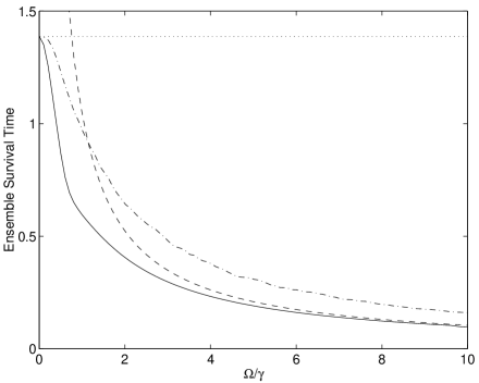
FIG. 3.: Plot of the ensemble survival time (in units of $\gamma^{-1}$) versus $\Omega/\gamma$. The solid curve is for the ensemble arising from direct detection (Sec. IV). The dashed curve is the large $\Omega/\gamma$ analytical approximation to it in Eq. (56). The dotted curve is that from the maximally robust unraveling (Sec. V). The dash-dot curve is that from the maximally robust continuous Markovian unraveling (Sec. VI). The unevenness in this final curve is due to statistical error in the ensemble averages $V_{v}$ and $V_{w}$), and gives an indication of the size of the statistical error.

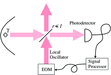
FIG. 4.: Diagram of the experimental configuration for an adaptive interferometric measurement of the fluorescence of an atom. The signal and a local oscillator are incident on a beam splitter of reflectance $r\ll 1$. The amplitude of the local oscillator is variable as a function of time, determined by an electro-optic modulator (EOM). The modulator is controlled by the experimenter, being inverted every time a detection occurs.

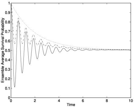
FIG. 5.: Plot of the ensemble average survival probability $S(t)$ versus time (in units of $\gamma^{-1}$) for the stationary ensembles of various detection schemes all with $\Omega/\gamma=10$. The three curves are for the minimally robust ($\upsilon=-1$) continuous Markovian unraveling (solid), the maximally robust ($\upsilon=1$) continuous Markovian unraveling (dash-dot) and the maximally robust unraveling (dotted).

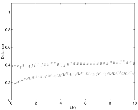
FIG. 6.: Plot of the distance of various ensembles from the maximally robust ensemble as a function of $\Omega/\gamma$. The solid line is for direct detection, which is the same as for continuous Markovian unraveling (CMU) with $\upsilon=-1$. The dashed line is for a CMU with $\upsilon=0$. The dash-dot line is for $\upsilon=1$ (the maximally robust CMU). In the latter two cases, the three lines indicate the mean, and the mean plus or minus one standard deviation (the statistical error in the ensemble average).