Cloning and quantum computation

Abstract

We discuss how quantum information distribution can improve the performance of some quantum computation tasks. This distribution can be naturally implemented with different types of quantum cloning procedures. We give two examples of tasks for which cloning provides some enhancement in performance, and briefly discuss possible extensions of the idea.

1 Introduction and overview

Since it became clear that it is impossible to make perfect copies of an unknown quantum state [1], much effort has been put into developing optimal cloning processes. As cloning represents a distribution of quantum information over a larger system, it can be seen as a type of quantum information processing tool. In this article we discuss the usefulness of quantum cloning to enhance the performance of some quantum computation tasks.

The COPY operation in classical computing is very useful, as it allows one to make multiple copies of the output of some computation, that can be fed as the input to further multiple processes. In quantum computing, however, the copying (quantum cloning) is imperfect, introducing some noise in the second round of computation. This situation is pictured in Fig. 1(a).

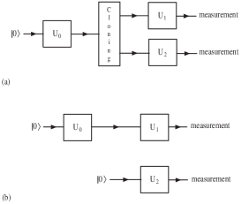
Figure 1: (a) This circuit represents the use of cloning to obtain information about computations $U_{1}U_{0}$ and $U_{2}U_{0}$ using $U_{0}$ only once. (b) This is one of the no-cloning strategies available for the same task. There are other possibilities: for example, we could embed each of the $U_{j}$ in a different quantum circuit, designed specifically for obtaining information about $U_{j}$.

We can represent the first part of the quantum computation as an unitary $U_{0}$ applied to the initial state $\left|0\right\rangle$, resulting in an output state that we clone. We then feed the clones to two different computational branches, represented by unitaries $U_{1}$ and $U_{2}$. At the end of the process we make a measurement on the two final states, obtaining some information about the two computational branches we want to perform ($U_{1}U_{0}\left|0\right\rangle$ and $U_{2}U_{0}\left|0\right\rangle$). The problem with this quantum scenario is that the copies are imperfect, resulting in lower chances of getting the correct results at the end. Nevertheless, we will show that at least for some tasks, the use of cloning improves our chances of correctly computing both branches, if there are constraints on the number of times we can run the first part $U_{0}$. In the two examples we discuss below we will be comparing approaches in which there is some distribution of quantum information (done by the cloning process) with any approach that does not resort to this (see Fig 1(b)).

We may discriminate between two main approaches to quantum cloning. The first relies on adding some ancillary quantum system in a known state and unitarily evolving the resulting combined system, deterministically obtaining a pure state with partial mixed density matrices $\rho_{c}$ (the clones) that are as close as possible to the original state $\left|\psi\right\rangle$, as measured by the fidelity $F=\left\langle\psi\right|\rho_{c}\left|\psi\right\rangle$ [2]. The clones are of the following form:

$$\rho_{c}=\frac{\mathbf{I}}{d}(1-\eta)+\eta\left|\psi\right\rangle\left\langle\psi\right|$$

Optimal universal cloning machines are the unitaries that result in the largest state-independent clone fidelities $F$. The efficiency of these machines have been shown to be characterized by [3]:

$$\eta =\frac{N}{M}\frac{\left(M+d\right)}{\left(N+d\right)}\quad;$$ (1)

$$F =\frac{(1-\eta)}{d}+\eta=\frac{M-N+N(M+d)}{M(N+d)}$$ (2)

where $d$ is the dimensionality of $\left|\psi\right\rangle$, $M$ is the number of clones and $N$ is the number of original copies of $\left|\psi\right\rangle$.

The second kind of cloning procedure is non-deterministic, consisting in adding an ancilla, performing unitary operations and measurements, with a postselection of the measurement results. Duan and Guo [4, 5] have shown that linearly independent pure states can be probabilistically cloned that way, and proved some theorems that allow one to calculate the optimal efficiencies. The resulting clones are perfect, but the procedure only succeeds with a certain probability $p<1$, which depends on the particular set of states which we are trying to clone.

Cloning machines can be viewed as a way of encoding quantum information contained in the input state $\left|\psi\right\rangle$ into a number of clones. In a sense, it accomplishes this more successfully than any procedure that relies on obtaining information about $\left|\psi\right\rangle$ through measurement. In order to see this, consider the universal cloning machines described above, operating on $N$ copies of $\left|\psi\right\rangle$, producing $M$ identical clones described by reduced density matrices $\rho_{c}$. Each clone has fidelity given by eq. 2; notice that the fidelity of the clones is a decreasing function of $M$. The best ‘classical clones’ that we can produce through measurement on $\left|\psi\right\rangle$ followed by state preparation have a lower fidelity, also given by 2, but with $M\rightarrow\infty$ [6, 7, 8]. It is in this sense that we can say that the cloning process distributes quantum information about $\left|\psi\right\rangle$ in a way that direct measurement on $\left|\psi\right\rangle$ cannot.

With these considerations in mind, it is natural to wonder if, and how, cloning can be used to improve the performance of quantum information processing tasks. One might think that cloning could be helpful in state estimation, but it has been shown that this task is equivalent to cloning, when the number of copies $M\rightarrow\infty$ [8, 9]. As a result, in order to obtain some improvement our strategy needs to rely on using the quantum information present in the clones for further coherent quantum information processing, in the same spirit as the circuit in Fig. 1a. In what follows we give two examples of tasks which can be better performed if we use quantum cloning. In the first example we apply optimal universal cloning machines, whereas in the second we rely on the probabilistic cloning discussed by Duan and Guo [4, 5].

2 Examples

In this section we present two examples of quantum computational tasks whose performance is enhanced if we distribute quantum information using quantum cloning. The first task makes use of state-independent universal quantum cloning, whereas the second task relies on state-dependent probabilistic quantum cloning.

2.1 First example

The first example we present is based on the scenario introduced in Fig. 1a. It models the general situation in which we want to perform $M$ different quantum computations, all of them with some first computational steps $U_{0}$ in common. Suppose that we are constrained to run $U_{0}$ only once. This may happen if $U_{0}$ is a complex, lengthy computation. In this case, we will be forced to find a scheme that obtains the $M$ computation results with the largest probability, using $U_{0}$ only once. Possible schemes may or may not resort to cloning to distribute quantum information; the example below is one in which cloning enables us to improve our performance, in relation to any scheme in which there is no information distribution using cloning.

In order to specify our task, suppose that we are given $(M+1)$ quantum blackboxes. What blackbox $j$ does is to accept one $d$-level quantum system as an input and apply a unitary operator $U_{j}$ to it, producing the evolved state as the output. We may think of the blackboxes as quantum oracles, or quantum sub-computations. The $U_{j}$ are chosen randomly from all possible $U(d)$ unitaries, using the unique uniform distribution invariant under action of $U(d)$ (see [10]). Our task will be to build quantum circuits that use each $U_{j}$ at most once to create $M$ mixed quantum states $\rho_{j}$, each as close as possible to $\left|\phi_{j}\right\rangle=U_{j}U_{0}\left|0\right\rangle,$ $(j=1,2,...M)$, where $\left|0\right\rangle$ is an arbitrary reference state. Our score will be given by the average fidelity of our guesses:

$$\overline{F}=\frac{1}{M}\sum_{j=1}^{M}\left\langle\phi_{j}\right|\rho_{j}\left|\phi_{j}\right\rangle.$$

If we are not allowed to clone the state, there are two possible strategies. The first no-cloning strategy is to start by finding one of the $\left|\phi_{j}\right\rangle$, say $\left|\phi_{1}\right\rangle=U_{1}U_{0}\left|0\right\rangle$, with fidelity one. Now that we have used $U_{0}$ and $U_{1}$ once already, we must make guesses about the other $(M-1)$ states $\left|\phi_{j}\right\rangle$ by using only the remaining $(M-1)$ blackboxes. As they were drawn from an uniformly random distribution, the best we can do is to make random guesses (each, on average, with $F=1/d$), obtaining, on average, a score

$$\bar{F}_{1}=\frac{1}{M}\left(1+\frac{(M-1)}{d}\right).$$

The second no-cloning strategy starts by running $U_{0}$ , followed by measurements that accomplish an optimal estimation of the resulting state $U_{0}\left|0\right\rangle$. After this, we can use the information gathered to build the $M$ imperfect copies necessary to proceed to the second part of the computation with the $U_{j}$ $(j=1,2,...M)$. As we have mentioned, this second approach yields clones with fidelity given by eq. 2 with $N=1,M\rightarrow\infty$  (see [8]):

$$\bar{F}_{2}=\frac{2}{(d+1)}.$$ (3)

We obtain our guesses for states $\left|\phi_{j}\right\rangle$ $(j=1,2,...M)$ by applying each $U_{j}$ $(j=1,2,...M)$ to a clone, resulting in a score also given by eq. 3. The best no-cloning strategy will be either of the two presented above, depending on the parameters $M$ and $d$.

Now let us see how cloning allows us to obtain a higher score $\overline{F}$ . We accomplish this by using a quantum circuit that first applies $U_{0}$ to the initial state $\left|0\right\rangle$, followed by an optimal universal cloning machine to obtain $M$ imperfect copies $\rho_{c}$ of state $U_{0}\left|0\right\rangle$. We then apply each $U_{j}$ $(j=1,2,...M)$ to a clone, obtaining reduced density matrices

$$\rho_{j}=\frac{\mathbf{I}}{d}(1-\eta)+\eta\left|\phi_{j}\right\rangle\left\langle\phi_{j}\right|$$

with $\eta$ given by eq. 1, with $N=1$. Using the resulting $\rho_{j}$’s as our guesses for states $\left|\phi_{j}\right\rangle$ $(j=1,2,...M)$, we obtain an overall score

$$\bar{F}_{cloning}=\frac{2M+d-1}{M(d+1)}$$ (4)

which is always higher than $\bar{F}_{1}$ and $\bar{F}_{2}$. In fact, eq. 4 represents the optimal score obtainable for this task, at least in the case $M=2$. In order to see this, we first note that asymmetric cloning (arising when the factors $\eta$ are in general different for each copy) is of no help in raising the score. This can be deduced from [11] and [12], where the authors consider asymmetric cloning with $M=2$ and show that the sum of the fidelities of the copies is maximized by symmetric cloning. Furthermore, the optimality of the universal cloning procedure we have used entails optimality for the fidelity of each of the $\rho_{j}$, and therefore a maximal value of the score $\bar{F}$. This shows that this task is optimally performed (with optimal score given by eq. 4) if and only if we are allowed to use cloning. It is straightforward to generalize the result to the case where we are allowed to run $U_{0}$ $N$ times $(N<M)$, instead of just once, and quantum cloning still offers an advantage.

The scenario described above models the situation in which we have a series of quantum computations with some computational steps $U_{0}$ in common. We must note that we have assumed complete lack of knowledge about the intermediate state $U_{0}\left|0\right\rangle$ and about the final target states $U_{j}U_{0}\left|0\right\rangle$ $(j=1,2,...M)$. In the general case this will not be a good assumption, as many quantum computations will output states picked from a limited set of states. This can be taken into account with state-dependent quantum cloning and a different choice of scoring functions. In the next section we give an example of this.

2.2 Second example

In our second example we take the blackboxes of the previous example to consist of arbitrary quantum circuits that query a given function only once. The query of function $f_{i}$ is the unitary that performs

$$\left|x\right\rangle\left|y\right\rangle\rightarrow\left|x\right\rangle\left|y\oplus f_{i}(x)\right\rangle,$$

where we have used the symbol $\oplus$ to represent the bitwise $XOR$ operation. For ease of analysis, we restrict ourselves to the case $M=2$ and also restrict the set of possible functions $f_{0}$, $f_{1}$ and $f_{2}$. Our task will involve determining two functionals, one which depends only on $f_{0}$ and $f_{1}$, and the other on $f_{0}$ and $f_{2}$. As in the previous example, we will compare the performances of cloning and no-cloning strategies.

In order to precisely state our task, let us start by considering all functions $h_{i}$ which take two bits to one bit. We may represent each such function with four bits $a,b,c$ and $d$, writing $h_{a,b,c,d}$ to represent the function $h$ such that $h(00)=a,h(01)=b,h(10)=c,$ and $h(11)=d$. Let us now define some sets of functions that will be helpful in stating our task:

$$S_{f0}=\{h_{0010},h_{0101},h_{1001}\},$$

$$S_{1}=\{h_{0001},h_{0010},h_{0100},h_{1000}\},S_{2}=\{h_{0000},h_{0011},h_{0101},h_{1001}\}$$

$$S_{f12}=S_{1}\cup S_{2},$$

$$S_{0000}=\{h_{0000},h_{1111}\},S_{0011}=\{h_{0011},h_{1100}\},$$ (5)

$$S_{0101}=\{h_{0101},h_{1010}\},S_{1001}=\{h_{1001},h_{0110}\},$$ (6)

$$S_{f}=S_{0000}\cup S_{0011}\cup S_{0101}\cup S_{1001}.$$

Now we randomly pick a function $f_{0}$ $\in S_{f0}$, after which two other functions $f_{1}$ and $f_{2}$ are picked from the set $S_{f12}$, also in a random fashion but obeying the constraints:

$$f_{0}\oplus f_{1}\quad,\quad f_{0}\oplus f_{2}\in S_{f}\quad.$$ (7)

Here we use the symbol $\oplus$ to represent addition modulo 2, which is equivalent to the bitwise $XOR$ operation. Our task will be to find in which of the four sets $S_{0000},S_{0011},S_{0101}$ and $S_{1001}$ lie each of the functions $f_{0}\oplus f_{1}$ and $f_{0}\oplus f_{2}$, using quantum circuits that query $f_{0},f_{1}$ and $f_{2}$ at most once each. Our score will be given by the average probability of successfully guessing both correctly.

The best no-cloning strategy we have found goes as follows. Firstly, note that if $f_{0}=h_{0010}$ then both $f_{1}$ and $f_{2}$ must be in set $S_{1}$, because of the constraints given by eq. 7; similarly, if $f_{0}$ is either $h_{0101}$ or $h_{1001}$, then $f_{1}$ and $f_{2}$ must be in set $S_{2}$. Since we have drawn the function $f_{0}$ randomly, we will have both functions $f_{1}$ and $f_{2}$ in set $S_{2}$ with probability $p=2/3$. We will assume that this is the case; then we can discriminate between the two possibilities for $f_{0}$ with a single, classical function call. Furthermore, by using the quantum circuit in Fig. 2 twice (once with each of $f_{1}$ and $f_{2}$) we can distinguish the four possibilities for functions $f_{1}$ and $f_{2}$.

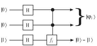
Figure 2: If function $f_{i}$ is guaranteed to be either in set $S_{1}$ or in $S_{2}$, then this quantum circuit can be used to distinguish between the four possibilities in each set. This is done by measuring the final state $\left|\phi_{i}\right\rangle=\sum_{x=00}^{11}(-1)^{f_{i}(x)}\left|x\right\rangle$ in one of two orthogonal bases, depending on which set contains $f_{i}$. The $H$ operations are Hadamard gates.

This happens because this quantum circuit results in four orthogonal states $\left|\phi_{i}\right\rangle=\sum_{x=00}^{11}(-1)^{f_{i}(x)}\left|x\right\rangle$, depending on which function in set $S_{2}$ was queried. This allows us to determine functions $f_{0},f_{1}$ and $f_{2}$ correctly with probability $p=2/3$, in which case we can determine which sets contain $f_{0}\oplus f_{1}$ and $f_{0}\oplus f_{2}$ and accomplish our task. Even in the case where our initial assumption about $f_{0}$ was wrong, we may still have guessed the right sets by chance; a simple analysis shows that our chances of getting both right this way are only $1/16$. On average, then, by using this no-cloning strategy we obtain a score:

$$p_{1}=\frac{2}{3}+\frac{1}{3}\cdot\frac{1}{16}=0.6875.$$

This is the best no-cloning score we could find for this task.

We can do better than that with quantum cloning. The idea now is to devise a quantum circuit that queries function $f_{0}$ only once, makes two clones of the resulting state and then queries functions $f_{1}$ and $f_{2}$, one in each branch of the computation. Since we have some information about the state produced by one query of $f_{0}$, the best cloning strategy will no longer be the universal, deterministic cloning derived in [2] ; the probabilistic cloning machines discussed by Duan and Guo [4], [5] will suit this task better.

The quantum circuit that we apply to solve this problem is given in Fig. 3.

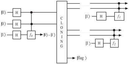
Figure 3: The cloning procedure in this circuit is probabilistic; a measurement on the state $\left|Flag\right\rangle$ tells us whether the cloning succeeded. If the cloning is successful we let the clones go through the rest of the circuit, yielding output states $\left|\phi_{i}\right\rangle=\frac{1}{4}\sum_{x=00}^{11}(-1)^{f_{0}(x)\oplus f_{i}(x)}\left|x\right\rangle$, $(i=1,2)$. These states can be measured in the basis defined by eqs. 13-16 to unambiguously decide which of the four sets $S_{0000},S_{0011},S_{0101}$ or $S_{1001}$ contains $f_{0}\oplus f_{i}$.

Immediately after querying function $f_{0}$, we have one of three possible linearly independent states (each corresponding to one of the possible $f_{0}$’s):

$$\left|h_{0010}\right\rangle \equiv\frac{1}{2}\left[\left|00\right\rangle+\left|01\right\rangle-\left|10\right\rangle+\left|11\right\rangle\right],$$ (8)

$$\left|h_{0101}\right\rangle \equiv\frac{1}{2}\left[\left|00\right\rangle-\left|01\right\rangle+\left|10\right\rangle-\left|11\right\rangle\right],$$ (9)

$$\left|h_{1001}\right\rangle \equiv\frac{1}{2}\left[-\left|00\right\rangle+\left|01\right\rangle+\left|10\right\rangle-\left|11\right\rangle\right].$$ (10)

We can build probabilistic cloning machines with different cloning efficiencies (defined as the probability of cloning successfully) for each of the states 8-10. Theorem 2 of [5] provides us with inequalities that allow us to derive achievable efficiencies for the probabilistic cloning process. We did a numerical search that yielded the following achievable efficiencies for probabilistically cloning the states in eqs. 8-10:

$$\gamma_{1} \equiv\gamma(\left|h_{0010}\right\rangle)=0.14165,$$ (11)

$$\gamma_{2} \equiv\gamma(\left|h_{0101}\right\rangle)=\gamma(\left|h_{1001}\right\rangle)=0.57122.$$ (12)

After the cloning process we can measure a ‘flag’ subsystem and know whether the cloning was successful or not. For this particular cloning process, the probability of success is, on average, $p_{\text{success}}=(\gamma_{1}+2\gamma_{2})/3\simeq 0.4280$. Let us suppose that it was successful. Then each of the cloning branches goes through the second part of the circuit in Fig. 3, to yield one of the four orthogonal states:

$$\left|h_{0000}\right\rangle \equiv\frac{1}{2}\left[\left|00\right\rangle+\left|01\right\rangle+\left|10\right\rangle+\left|11\right\rangle\right],$$ (13)

$$\left|h_{0011}\right\rangle \equiv\frac{1}{2}\left[\left|00\right\rangle+\left|01\right\rangle-\left|10\right\rangle-\left|11\right\rangle\right],$$ (14)

$$\left|h_{0101}\right\rangle \equiv\frac{1}{2}\left[\left|00\right\rangle-\left|01\right\rangle+\left|10\right\rangle-\left|11\right\rangle\right],$$ (15)

$$\left|h_{1001}\right\rangle \equiv\frac{1}{2}\left[-\left|00\right\rangle+\left|01\right\rangle+\left|10\right\rangle-\left|11\right\rangle\right],$$ (16)

which can be discriminated unambiguously. We obtain state $\left|h_{0000}\right\rangle$ if and only if the combined function $f_{0}\oplus f_{i}$ is one of the two in set $S_{0000}$, as can be checked by calculating the effect of the circuit in Fig. 3 for all possible $f_{0},f_{1}$ and $f_{2}$. The situation is similar for the other three states; the detection of each of them signals precisely which one of the four sets $\{S_{0000},S_{0011},S_{0101},S_{1001}\}$ contains $f_{0}\oplus f_{i}$ . As a result, if the cloning process is successful, we manage to accomplish our task.

However, the cloning process will fail with probability $(1-p_{\text{success}})$. If this happens, a simple evaluation of the posterior probabilities for function $f_{0}$ shows that it is more likely to be $h_{0010}$ than the other two, thanks to the relatively low cloning efficiency for  the state in eq. 8, in relation to the states in eqs. 9 and 10 (see eqs. 11-12). If we then guess that $f_{0}=h_{0010}$, we will be right with probability

$$p_{0010}=\frac{(1-\gamma_{1})}{(1-\gamma_{1})+2(1-\gamma_{2})}\simeq 0.5002.$$

What is more, we are still free to design quantum circuits to obtain information about $f_{1}$ and $f_{2}$, since at this stage we still have not queried them. Given our guess that $f_{0}=h_{0010}$, only the four functions in $S_{1}$ can be candidates for $f_{1}$ and $f_{2}$, because of the constraints given by eq. 7. These four possibilities can be discriminated unambiguously by running a circuit like that of Fig. 2 twice, once with $f_{1}$ and once with $f_{2}$. The circuit produces one of four orthogonal states, each corresponding to one of the four possibilities for $f_{i}$. Therefore, if our guess that $f_{0}=h_{0010}$ was correct, we are able to find the correct $f_{1}$ and $f_{2}$ and therefore accomplish our task. In the case that $f_{0}\neq h_{0010}$ after all, we may still have guessed the right sets by chance; a simple analysis shows that this will happen with probability $1/16$.

The above considerations lead to an overall probability of success given by

$$p_{2}=p_{\text{success}}+(1-p_{\text{success}})\left[p_{0010}+(1-p_{0010})\frac{1}{16}\right]\simeq 0.7320>p_{1}=0.6875,$$

thus showing that our cloning approach is more efficient than the previous one, which does not use cloning. We have not proven that the first approach is the most efficient among those that do not resort to cloning, but we conjecture that it is.

Besides this larger probability of obtaining the correct result, our cloning approach offers another advantage: the measurement of the ‘flag’ state allows us to be confident about having the correct result in a larger fraction of our attempts. For the probabilistic cloning machines described above this fraction was $\simeq 0.428$, but  this can be improved by choosing a different cloning machine, characterized by $\gamma_{1}=0.3485,\gamma_{2}=0.5258$. This latter machine signals a guaranteed correct result in a fraction $(\gamma_{1}+2\gamma_{2})/3\simeq 0.467$ of the runs. The best no-cloning approach for obtaining these guaranteed correct results would involve unambiguous discrimination of the function $f_{0}$, followed by the distinction among the four possibilities for functions $f_{1}$ and $f_{2}$ (this second step is simple if we know $f_{0}$ for certain). Theorem 4 of [5] provides us with a tool to numerically determine the best efficiency for unambiguous discrimination of $f_{0}$. A numerical search indicates that this can be done only with efficiency $\leq 1/3$, and therefore this is the limit for the fraction of runs for which we can obtain a guaranteed correct result for the task at hand, if we do not resort to cloning.

3 Conclusion

We have given two examples of tasks whose performance is enhanced by the use of quantum cloning. As we have discussed, cloning may offer advantages for a whole class of quantum computational tasks. Cloning need not be made only once during the course of a computation; nor does it necessarily need be one of the two kinds discussed above. For example, asymmetric cloning [11] may also be useful, depending on the nature of the task at hand.

We must note that general quantum algorithms already manipulate quantum information, distributing it among different parts of the quantum register during a computation. What we have shown here is that quantum cloning can be taken as a natural quantum information processing tool to do this quantum information distribution, in order to optimize our use of computational resources. It would be interesting to find other tasks that could profit from cloning, perhaps by combining already known quantum algorithms with some intermediate cloning steps.

In this paper we have not discussed how the cloning circuit complexity scales with input size. Some authors have developed quantum circuits for deterministically cloning single qubits [13, 14], and networks for state-dependent cloning [15]. Further work on circuits for deterministically cloning $d$-dimensional systems ($d>2$) is still required.

4 Acknowledgments

We acknowledge support from the Royal Society, the ORS Award Scheme and the Brazilian agency Coordenação de Aperfeiçoamento de Pessoal de Nível Superior (CAPES).

References

- [1] W. K. Wootters and W. H. Zurek, Nature 299, 802 (1982).
- [2] V. Bužek and M. Hillery, Phys. Rev. A 54, 1844 (1996).
- [3] R. Werner, Phys. Rev. A 58, 1827 (1998).
- [4] L.-M. Duan and G.-C. Guo, Los Alamos e-print archive quant-ph/9705018.
- [5] L.-M. Duan and G.-C. Guo, Phys. Rev. Lett. 80, 4999 (1998).
- [6] S. Massar and S. Popescu, Phys. Rev. Lett. 74, 1259 (1995).
- [7] N. Gisin and S. Massar, Phys. Rev. Lett. 79, 2153 (1997).
- [8] D. Bruß and C. Macchiavello, Phys. Lett. A 253, 249 (1999).
- [9] D. Bruß, A. Ekert and C. Macchiavello, Phys. Rev. Lett. 81, 2598 (1998).
- [10] E. Lubkin, J. Math. Phys. 19, 1028 (1978).
- [11] V. Bužek, M. Hillery and R. Bednik, Acta Phys. Slov. 48, 177 (1998).
- [12] N. Cerf, J. Mod. Opt. 47, 187 (2000).
- [13] V. Bužek, S. L. Braunstein, M. Hillery, D. Bruß, Los Alamos e-print archive quant-ph/9703046.
- [14] V. Bužek, M. Hillery, Los Alamos e-print archive quant-ph/9801009.
- [15] A. Chefles, S. M. Barnett, Los Alamos e-print archive quant-ph/9812035.