Abstract

The spectroscopic properties of an open quantum system are determined by the eigenvalues and eigenfunctions of an effective Hamiltonian ${\cal H}$ consisting of the Hamiltonian ${\cal H}_{0}$ of the corresponding closed system and a non-Hermitian correction term $W$ arising from the interaction via the continuum of decay channels. The hermitian part of ${\cal H}$ is ${\cal H}_{0}+\Re(W)$ while the anti-hermitian part is $\Im(W)$. This holds for a many-particle system as well as for a microwave resonator. The eigenvalues ${\cal E}_{R}$ of ${\cal H}$ are complex. They are the poles of the $S$-matrix and provide both the energies and widths of the states. We illustrate the interplay between $\Re({\cal H})$ and $\Im({\cal H})$ by means of the different interference phenomena between two neighboured resonance states. Level repulsion along the real axis appears if the interaction is caused mainly by (the non-diagonal part of) $\Re({\cal H})$ while a bifurcation of the widths appears if the interaction occurs mainly due to (the non-diagonal part of) $\Im({\cal H})$. We then calculate the poles of the $S$-matrix and the corresponding wavefunctions for a rectangular microwave resonator with a scatter as a function of the area of the resonator as well as of the degree of opening to a guide. The calculations are performed by using the method of exterior complex scaling. $\Re(W)$ and $\Im(W)$ cause changes in the structure of the wavefunctions which are permanent, as a rule. At full opening to the lead, short-lived collective states are formed together with long-lived trapped states. The wavefunctions of the short-lived states at full opening to the lead are very different from those at small opening. The resonance picture obtained from the microwave resonator shows all the characteristic features known from the study of many-body systems in spite of the absence of two-body forces. The poles of the $S$-matrix determine the conductance of the resonator. Effects arising from the interplay between resonance trapping and level repulsion along the real axis are not involved in the statistical theory (random matrix theory).

1 Introduction

Since more than ten years, interference phenomena in open quantum systems are studied theoretically in the framework of different models. Common to all these studies is the appearance of different time scales as soon as the resonance states start to overlap (see [1, 2, 3, 4, 5, 6, 7, 8] and references in these papers to older ones). Some of the states align with the decay channels and become short-lived while the remaining ones decouple to a great deal from the continuum of decay channels and become long-lived. The wavefunctions show permanent changes: they are mixed strongly in the basic wavefunctions of the corresponding closed system.

In many-body systems the interaction is caused, above all, by two-body forces between the constituents of the system. The additional interaction connected with avoided level crossings is believed, usually, to lead only to an exchange of the wavefunctions but not to permanent changes of their structure. This conclusion results from many spectroscopic studies on closed systems with discrete states. Recent investigations in the framework of a schematical model [1] showed however that, in the case of collective resonance states, permanent changes in the wavefunctions occur due to the interplay between the real and imaginary parts of the different coupling matrix elements.

The mixing of the resonance states of a microwave resonator is not caused by two-body forces. A mixing of the states may occur only as a result of avoided level crossings. It is therefore an interesting question whether or not some permanent mixing in the wavefunctions of a microwave cavity can arise. In [9], the changes in the structure of the wavefunctions at avoided crossings in a strongly driven (closed) square potential well system are studied. The avoided crossings are shown to lead, in some cases, to temporary and, in other cases, to permanent changes as a function of driving field strength.

The avoided level crossings are related to exceptional points in the complex plane [6]. The coupling induced by avoided level crossings is therefore surely connected with the coupling matrix elements of the discrete states of the closed system to the continuum. In the continuum shell model, these coupling matrix elements are complex [10]. Interferences appear when more than one channel are open. It is possible therefore that interferences of different type may provide eventually a permanent mixing of the wavefunctions of the resonance states. A similar study for microwave cavities does not exist.

It is the aim of the present paper to study the resonance picture of an open microwave resonator in detail. We show that its characteristic features are the same as those which are known from open many-body quantum systems. This means that not only two-body forces play a role for the interaction among the resonance states but also the interaction $W$ via the continuum is important. Neither $\Re(W)$ nor $\Im(W)$ can be neglected, generally. They are important near avoided crossings in the complex plane and their interplay can not be neglected when $\Re(W)$ and $\Im(W)$ are of the same order of magnitude. As a result, permanent changes in the structure of the wavefunctions appear, as a rule. The basic assumptions of the statistical theory (random matrix theory) are fulfilled only when the interferences caused by the hermitian and anti-hermitian parts of the Hamiltonian can be neglected to a good approximation. This is the case e.g. for a Gaussian orthogonal ensemble coupled weakly to the continuum.

In Section 2 of the present paper, the Hamiltonian of an open quantum system and the relation of its eigenvalues to the poles of the $S$-matrix is considered. The formalism can be applied to a many-body system as well as to a microwave resonator. The Hamiltonian is non-hermitian and the eigenvalues provide the energies as well as the widths of the states. In Section 3, the avoided crossing of two resonance states is traced. The differences between the mixing of the states due to the hermitian and the anti-hermitian part of ${\cal H}$ are the central point of discussion. The hermitian part causes an equilibration of the states in relation to the time scale which is accompanied by level repulsion along the real axis (energy). In contrast to this, the anti-hermitian part leads to an attraction of the levels in energy and to a bifurcation of the widths (formation of different time scales). These processes are characteristic for the interplay among resonances which takes place locally in more complicated systems [11].

In Section 4, the resonance structure of a rectangular microwave resonator coupled to one lead is studied. Inside the resonator is a circular scatter. Level repulsion in the complex plane appears. It can be seen sometimes as level repulsion along the real energy axis. In other cases, a bifurcation of the widths occurs. The changes in the structure of the wavefunctions are permanent, as a rule. Collective states are formed at strong coupling to the lead. The structure of their wavefunctions has almost nothing in common with the structure of the wavefunctions of these states at small coupling. Together with the collective states, long-lived trapped states appear. The conductance of the microwave resonator is studied after coupling it to a second lead. The conductance peaks are determined by the poles of the $S$-matrix, which move as a function of the coupling strength between cavity and leads. The results are discussed in Section 5 and some conclusions are drawn in the last section.

2 The Hamilton operator of an open quantum system

The function space of an open quantum system consists of two parts: the subspace of discrete states ($Q$-subspace) and the subspace of scattering states ($P$-subspace). The discrete states are the states of the closed system which are embedded into the continuum of scattering states. Due to the coupling of the discrete states to the continuum, they can decay and get a finite lifetime.

Let us define two sets of wavefunctions by solving first the Schrödinger equation $(H^{\rm cl}-E_{R}^{\rm cl})\;\Phi_{R}^{\rm cl}=0$ for the discrete states of the closed system and secondly the Schrödinger equation $(H^{cc}-E^{(+)})\;\xi_{E}^{c}=0$ for the scattering states of the environment. Note that the closed system can be a many-particle quantum system or a system like a microwave resonator. The only condition is that it can be described quantum mechanically by the hermitian Hamilton operator $H^{\rm cl}$. In the case of the flat microwave resonator, this is possible by using the analogy to the Helmholtz equation. Then, the $Q$ and $P$ operators can be defined by

$$Q=\sum_{R=1}^{N}\;|\Phi_{R}^{\rm cl}\rangle\langle\Phi_{R}^{\rm cl}|\;\qquad P=\sum_{c=1}^{\Lambda}\int_{\epsilon_{c}}^{\infty}\;dE\;\;|\xi_{E}^{c}\rangle\langle\xi_{E}^{c}|$$ (1)

and $Q\cdot\xi_{E}^{c}=0\,;\;P\cdot\Phi_{R}^{\rm cl}=0$. In order to perform spectroscopic studies, we do not use any statistical assumptions (for details see [12]).

Assuming $Q+P=1$, we can determine a third wavefunction by solving the scattering problem $(H^{cc}-E^{(+)})\;\omega_{R}=-\sum_{c}\gamma_{Rc}\;\xi_{E}^{c}$ with source term. The source term is determined by the coupling matrix elements $\gamma_{Rc}$ between the two subspaces. Further, we identify $H^{\rm cl}$ with ${\cal H}_{0}\equiv QHQ$ where $(H-E)\Psi=0$ is the Schrödinger equation in the total function space $P+Q$. Then, the solution $\Psi=P\Psi+Q\Psi$ in the total function space is [12]

$$\Psi = \xi_{E}^{c}+\frac{1}{2\pi}\sum_{R=1}^{N}\sum_{R^{\prime}=1}^{N}(\Phi_{R}^{\rm cl}+\omega_{R})\cdot\langle\Phi_{R}^{\rm cl}|\frac{1}{E-{\cal H}}|\Phi_{R^{\prime}}^{\rm cl}\rangle\;\gamma_{R^{\prime}c}$$ (2)

$$= \xi_{E}^{c}+\sum_{R=1}^{N}{\tilde{\Phi}}_{R}\cdot\frac{\tilde{\gamma}_{Rc}}{E-{\tilde{E}}_{R}+\frac{i}{2}{\tilde{\Gamma}}_{R}}\;.$$

Here,

$${\cal H}={\cal H}_{0}+W$$ (3)

is the effective Hamilton operator appearing in the $Q$-subspace due to the coupling to the continuum, ${\tilde{\Phi}}_{R}$ are the eigenfunctions of ${\cal H}$ and $\tilde{\cal E}_{R}\equiv{\tilde{E}}_{R}-\frac{i}{2}\;{\tilde{\Gamma}}_{R}$ its eigenvalues. They provide the wavefunctions, energies and widths, respectively, of the resonance states. The $\gamma_{Rc}$ are the coupling matrix elements between the discrete states $\Phi_{R}^{\rm cl}$ and the continuum of scattering states $\xi_{E}^{c}$, while the $\tilde{\gamma}_{Rc}$ are those between the resonance states $\tilde{\Phi}_{R}$ and the continuum. The matrix elements of $W$ consist of the principal value integral and the residuum [12],

$$W_{R^{\prime}R}^{\rm ex} = \frac{1}{2\pi}\sum_{c=1}^{\Lambda}{\cal P}\int\limits_{\epsilon_{c}}^{\infty}dE^{\prime}\;\frac{\gamma_{Rc}\;\gamma_{R^{\prime}c}}{E-E^{\prime}}\;-\;\frac{i}{2}\sum_{c=1}^{\Lambda}\gamma_{Rc}\;\gamma_{R^{\prime}c}\;.$$ (4)

Here, $c=1,...,\Lambda$ are the channels which open at the energies $\epsilon_{c}$. They describe the external mixing of two states via the continuum of decay channels. As a rule, both parts $\Re(W)$ and $\Im(W)$ are non-vanishing.

Note, the expressions (2), (3) and (4) follow by formal rewriting the Schrödinger equation $(H-E)\Psi=0$ with the only condition that $Q$ and $P=1-Q$ are defined in such a manner that the channel wavefunctions of the $P$ subspace are uncoupled [12]. Otherwise, the eigenvalues and eigenfunctions of ${\cal H}$ have no physical meaning. The $\tilde{E}_{R},\;\tilde{\Gamma}_{R},\;\tilde{\gamma}_{Rc}$ and $\tilde{\Phi}_{R}$ are energy dependent functions, generally.

The resonance part of the $S$-matrix is [12]

$$S_{cc^{\prime}}^{(\rm res)}=i\sum_{R=1}^{N}\frac{\tilde{\gamma}_{Rc^{\prime}}\tilde{\gamma}_{Rc}}{E-{\tilde{E}}_{R}+\frac{i}{2}{\tilde{\Gamma}}_{R}}\;.$$ (5)

We underline that the $\tilde{\gamma}_{Rc},~{}\tilde{E}_{R}$, $\tilde{\Gamma}_{R}$ and $\tilde{\Phi}_{R}$ are functions which are calculated inside the formalism. They contain the contributions of $\Im(W)$ and of $\Re(W)$. The $\tilde{\gamma}_{Rc}$ and $\tilde{\Phi}_{R}$ are complex.

3 Avoided crossing of two resonance states

3.1 Schematical study

In order to illustrate the mutial influence of two neighboured resonance states, we consider the following Hamilton operator

$${\cal H}^{(v)} = \left(\begin{array}[]{cc}\epsilon_{1}&v_{\rm in}\\ v_{\rm in}&\epsilon_{2}\end{array}\right)\equiv\left(\begin{array}[]{cc}E_{1}&v_{\rm in}\\ v_{\rm in}&E_{2}\end{array}\right)-\frac{i}{2}\;\left(\begin{array}[]{cc}\Gamma_{1}&0\\ 0&\Gamma_{2}\end{array}\right)$$ (12)

which describes two resonance states lying at the energies $E_{1}$ and $E_{2}$. These two states have the widths $\Gamma_{1}$ and $\Gamma_{2}$, respectively, and are coupled by $v_{\rm in}$ (where $v_{\rm in}$ is real). The eigenvalues are:

$${\cal E}_{\pm}^{(v)}=\frac{\epsilon_{1}+\epsilon_{2}}{2}\pm\frac{1}{2}\;\sqrt{(\epsilon_{1}-\epsilon_{2})^{2}+4v_{\rm in}^{2}}\;.$$ (13)

When $\Gamma_{1}\approx\Gamma_{2}$, the coupling $v_{\rm in}$ of the two states leads to level repulsion along the real axis. Numerical results for $\Gamma_{1}\not\approx\Gamma_{2}$ are shown in Figure 1.a.

Let us now consider the Hamiltonian with the coupling $iw_{\rm ex}$ ($w_{\rm ex}$ is real) of the two states via the continuum,

$${\cal H}^{(w)} = \left(\begin{array}[]{cc}\epsilon_{1}&i\;w_{\rm ex}\\ i\;w_{\rm ex}&\epsilon_{2}\end{array}\right)\equiv\left(\begin{array}[]{cc}E_{1}&0\\ 0&E_{2}\end{array}\right)\;-\frac{i}{2}\;\left(\begin{array}[]{cc}\Gamma_{1}&-2w_{\rm ex}\\ -2w_{\rm ex}&\Gamma_{2}\end{array}\right)\;.$$ (20)

In this case, the eigenvalues are:

$${\cal E}_{\pm}^{(w)}=\frac{\epsilon_{1}+\epsilon_{2}}{2}\pm\frac{1}{2}\;\sqrt{(\epsilon_{1}-\epsilon_{2})^{2}-4w_{\rm ex}^{2}}\;.$$ (21)

For $E_{1}\approx E_{2}$, the coupling via the continuum due to $iw_{\rm ex}$ leads to repulsion along the imaginary axis (bifurcation of the widths), i.e. to resonance trapping. Numerical results for $E_{1}\not\approx E_{2}$ are shown in Figure 1.d.

As it is well known and can be seen from eq. (13), two interacting discrete states ($v_{\rm in}\neq 0$) can not cross. In the complex plane, however, the conditions for crossing of two resonance states may be fulfilled. From ${\cal E}_{+}={\cal E}_{-}$, it follows

$$R \equiv (E_{1}-E_{2})^{2}-\frac{1}{4}(\Gamma_{1}-\Gamma_{2})^{2}+4(v_{\rm in}^{2}-w_{\rm ex}^{2})=0$$

$$I \equiv (E_{1}-E_{2})(\Gamma_{1}-\Gamma_{2})+8v_{\rm in}w_{\rm ex}=0$$ (22)

for the general case of a complex interaction $v_{\rm in}+iw_{\rm ex}$. These conditions define the critical values of the coupling strength ($v_{\rm in}^{\rm cr}$ and $w_{\rm ex}^{\rm cr}$, respectively) at which the $S$-matrix has a branch point [13].

It is also possible that two resonance states cross along the real or imaginary axis while the crossing is avoided along the other axis. The conditions for such a case with $I=0$ are $R<0$ for crossing along the real axis and $R>0$ for crossing along the imaginary axis. The crossing in the complex plane is avoided, in any case.

The trajectories for the motion of the eigenvalues in the complex plane as a function of the interaction $v_{\rm in}$ and $w_{\rm ex}$, respectively, (Figures 1.a and d) show the avoided crossing of the two resonance states in the complex plane. It occurs at a certain critical value of the coupling strength. Here and in its neighbourhood a redistribution between the two states takes place. It is accompanied by the biorthogonality of the eigenfunctions $\tilde{\Phi}_{i}$ of ${\cal H}$, $\;B\equiv(1/2)\sum_{i=1,2}\langle\tilde{\Phi}_{i}|\tilde{\Phi}_{i}\rangle>1$. The wavefunctions of the two resonance states become mixed: $\tilde{\Phi}_{i}=\sum b_{ij}\Phi_{j}^{0}$ where the $\Phi_{j}^{0}$ are the eigenfunctions of ${\cal H}^{0}$, which is the Hamilton operator with vanishing non-diagonal matrix elements ($v_{\rm in}=0$ and $w_{\rm ex}=0$, respectively). In Figures 1.b, c and e, f, the coefficients $b_{ij}$ are shown as a function of the coupling strength $v_{\rm in}$ and $w_{\rm ex}$, respectively.

The results can be summarized in the following manner.

• Weak interaction $v_{\rm in}<v_{\rm in}^{\rm cr}$ or $w_{\rm ex}<w_{\rm ex}^{\rm cr}$:
  the resonance states are isolated, their positions and widths are almost independent of the value of $v_{\rm in}$ and $w_{\rm ex}^{\rm cr}$, respectively.
  $B\approx 1$.
  

• Starting at a certain critical value of the coupling strength, the behaviour of the system is different for the two cases with $v_{\rm in}$ and $w_{\rm ex}$.
  $v_{\rm in}\approx v_{\rm in}^{\rm cr}$: the states start to repel in energy and to attract each other along the imaginary axis (if their widths at small $v_{\rm in}$ are different).
  $w_{\rm ex}\approx w_{\rm ex}^{\rm cr}$: the widths bifurcate and the levels attract each other along the real axis (if their positions in energy at small $w_{\rm ex}$ are different).
  In both cases $B\gg 1$. The wavefunctions of the two states become mixed.
  

• $v_{\rm in}>v_{\rm in}^{\rm cr}$: the widths are almost independent of $v_{\rm in}$: (equilibration in relation to the time scale) and the states repel each other along the real axis (level repulsion).
  $w_{\rm ex}>w_{\rm ex}^{\rm cr}$: the energies are almost independent of $w_{\rm ex}$ (the two states remain close to one another in their position) and resonance trapping occurs (the width of one of the states increases with increasing $w_{\rm ex}$, while the width of the other state decreases).
  In both cases $B\to 1$.

From a mathematical point of view, the properties of the system at an avoided crossing in the complex plane (i.e. in the region of the critical coupling strength $v_{\rm in}^{\rm cr}$ and $w_{\rm ex}^{\rm cr}$, respectively) are almost the same: repulsion of the eigenvalues along one axis and attraction along the other axis. The physical meaning is, however, very different: $v_{\rm in}$ causes equilibrium (in relation to the lifetime) and level repulsion along the real axis while $iw_{\rm ex}$ creates different time scales (bifurcation of the widths) and level attraction along the real axis.

When the coupling contains both $v_{\rm in}$ and $iw_{\rm ex}$, then it depends on the ratio between the two parts whether level repulsion or attraction along the real axis dominates. In any case, the crossing of states is avoided in the complex plane and results in a complicated interference picture. The wavefunctions of the resonance states are mixed permanently in the set of the eigenfunctions of the Hamiltonian ${\cal H}^{0}$ of the corresponding closed system.

3.2 Realistic cases

In [7], the behaviour of poles of the $S$-matrix in an open two-dimensional regular microwave billiard connected to a single waveguide is studied. As a function of the coupling strength between the resonator and the waveguide, the position of the correponding resonance poles, the wavefunctions of the resonance states and the Wigner-Smith time delay function are calculated. The poles are calculated on the basis of the exterior complex scaling method. The energy of the incoming wave is chosen so that only the channel corresponding to the first transversal mode in the lead is open.

In [7], the bifurcation of the widths (resonance trapping) can be seen very clearly, indeed. In particular, the contraintuitive result that the lifetimes of certain resonance states increase with increasing coupling to the continuum can be traced not only in the motion of the poles of the $S$-matrix in the complex plane. It can be seen also in the wavefunctions of the resonance states and, above all, in the measurable time-delay function. In the case of three interfering resonance states, the wavefunction of (at most) one of the long-lived trapped states may be pure in relation to the bound states of the closed resonator [7]. More exactly: $b_{ii}=1$ at small and large coupling strength. Some mixing of all three wavefunctions appears in the critical region where the wavefunctions are biorthogonal ($B>1$).

Another example is the motion of the poles of the $S$-matrix by varying the coupling strength between the states of an atom by means of a laser. In [3], the positions and widths of two resonances in the vicinity of an autoionizing state coupled to another autoionizing one (or a discrete state) by a strong laser field are considered. For different atomic parameters, the trajectories in the complex energy plane are traced by fixing the field frequency $\omega$ but varying the intensity $I$ of the laser field. The states are coupled directly as well as via a common continuum and the ratio of these couplings is defined by the Fano parameter $Q$ [15]. Most interesting is the region of avoided resonance crossing where the motion of each eigenvalue trajectory is influenced strongly by the motion of the other one. This occurs at a certain critical intensity $I_{\rm cr}$. When furthermore the frequency is equally to the critical value $\omega_{\rm cr}$, then laser induced degenerate states arising at the double pole of the $S$-matrix are formed. The strong correlation between the two states for intensities around $I_{\rm cr}$ reflects itself in the strong changes of the shape parameters of the resonances in the cross section. It can therefore be traced.

In the limit of vanishing direct coupling ($Q\to 0$), the widths bifurcate at $I=I_{\rm cr}$ as in other open quantum systems. That means, the width of one of the resonance states increases with increasing $I>I_{\rm cr}$ while the width of the other decreases relatively to the first one. In the limit $I\to\infty$, the ratio between the width of the long-lived and short-lived state approaches zero (resonance trapping). This corresponds to the situation shown in Fig. 1.d. In the other limiting case, the coupling via the continuum vanishes ($Q$ value large). Here, the levels repel in their energetic positions when $I\geq I_{\rm cr}$. This corresponds to Fig. 1.a.

In any case, i.e. for all $Q$ values, the two resonance states start to repel each other in the complex energy plane at $I=I_{\rm cr}$. The repulsion of the eigenvalues in the complex plane is an expression of the strong mutual influence of one state on the other one in the critical region around $I_{\rm cr}$. In the transition region ($Q$ values of the order of magnitude 1), the trajectories show a complicated behaviour. Here, population trapping may appear, i.e. the width of one of the resonance states may vanish at a certain finite intensity $I_{\rm pt}>I_{\rm cr}$. It appears, generally, if the process is neither pure level repulsion on the real axis nor pure resonance trapping but the amplitudes of both processes (i.e. the direct coupling of the two states and their coupling via the continuum) are of comparable importance and interfere.

Thus, the results obtained in [3] for two interacting atomic levels confirm qualitatively the results of the schematical study represented in Section 3.1, although not only the non-diagonal matrix elements of $H^{\rm eff}$ but also the width $\Gamma_{1}$ itself depends on $I$. These results and those for the microwave cavity discussed above show very clearly that individual resonance states can mix not only due to the two-body forces between the substituents of the system but also as a consequence of avoided resonance crossings.

Other realistic cases are considered in [14]. These are the resonance doublet $J^{\pi}=2^{+},\;T=0,\;1$ in the nucleus ⁸Be and the $\rho-\omega,\;T=1,\;0$ doublet of mesons.

4 Spectroscopic properties of an open microwave resonator

4.1 Calculations for the open microwave resonator

The calculations are performed for a rectangular flat resonator coupled to a waveguide. Inside the cavity, a circular scatter is placed. We use the Dirichlet boundary condition, $\Phi=0$, on the border of the billiard and of the waveguide. The waveguide has a width equal to $1$ and is attached to the resonator through a slide with an adjustable opening (which is described also by the Dirichlet boundary condition). For $w=0.5$ the resonator and the waveguide are disconnected, while $w=0$ represents the maximal coupling (opening).

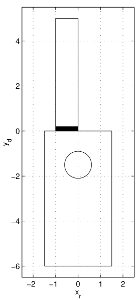
Figure 2: The resonator. The slide, shown in black, will be opened from the center to both sides (0.5 $\geq w\geq$ 0, where $w$ = 0.5 (0) corresponds to closed (fully open)). $x_{r}$ and $y_{d}$ are given in arbitrary units $[x]$.

The cavity has a minimum area $3\times 3$ which is determined by $x_{r}=1.5$ and $y_{d}=-3$ (compare Figure 2). The area is varied by varying $x_{r}$ or $y_{d}$ while both the position of the lead and the scatter inside the cavity remain unchanged.

We solve the equation $-\Delta\Phi=E\Phi\;.$ Inside the waveguide, the wavefunction has the asymptotic form $\Phi=\left(e^{iky}-R(E)e^{-iky}\right)u(x)\;.$ Here $u(x)$ is the transversal mode in the waveguide, $k$ is the wave number and $R(E)$ is the reflection coefficient. The energies and widths of the resonance states are given by the poles of the coefficient $R(E)$ analytically continued into the lower complex plane. They are identical to the poles of the $S$ matrix when the fixed point equations for the $\tilde{E}_{R}$ and $\tilde{\Gamma}_{R}$ are solved (see Section 2).

To find the poles we use the method of exterior complex scaling [16, 17]. For details see [8].

4.2 Resonances as a function of the area of the resonator

We studied the motion of the poles of the $S$ matrix as a function of the area of the resonator by changing both its length $y$ and width $x$. The changes of the corresponding wavefunctions $\Phi_{R}$ are traced. We studied the energy region between the two thresholds at $\pi^{2}\approx 10$ and $(2\pi)^{2}\approx 40$ where only one channel is open.

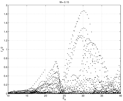
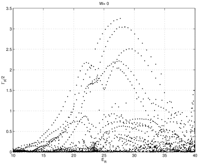
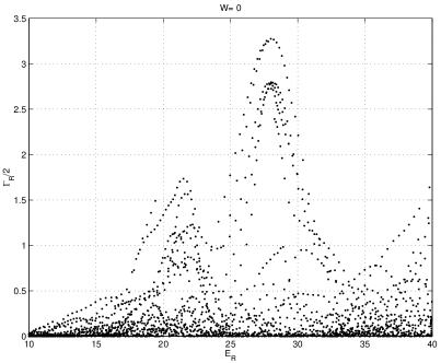
Figure 3: Eigenvalue picture: motion of the poles of the $S$-matrix in dependence on increasing length (left) ($y_{d}$ = -6.0 : 0.02 : -3.0; $x_{r}$ = 1.5) and width (right) ($x_{r}$ = 1.5 : 0.02 : 3.5; $y_{d}$ = -3.0) of the resonator. The opening of the aperture is $w$ = 0.15 (top) and $w$ = 0 (bottom). The energies are given in units of $[x]^{-2}$.

In Figure 3, the eigenvalue picture is shown for $w=0.15$ (aperture partly closed by the slide) and $w=0$ (aperture fully open) for different values of the length and width of the resonator. In all cases, oscillations of the widths as a function of $y_{d}$ or $x_{r}$ in the energy region considered can be seen. The amplitudes of the oscillations are larger for larger widths. At $w=0.15$, all states corresponding to different $y_{d}$  ($-3>y_{d}>-6$) and lying around 24 have small widths. This is caused, obviously, by certain symmetry properties of the wavefunctions in relation to the channel (since this energy is in the middle between the two thresholds). The minimum in the widths vanishes when the wavefunctions are strongly mixed via the continuum ($w=0$). This shows that the coupling to the channel washes out some spectroscopic properties of the closed system.

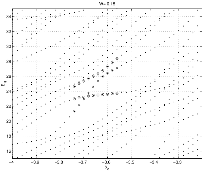
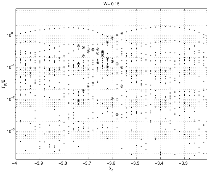
Figure 4: Energies (top) and widths (bottom) as a function of $y_{d}$ for $w=0.15$ and $x_{r}$ = 1.5. For 10 values of $y_{d}$, the poles of three states are marked by diamonds (A), stars (B) and circles (C). It is $E_{A}>E_{B}>E_{C}$ and $\Gamma_{B}>\Gamma_{C}>\Gamma_{A}$ at $y_{d}$ = -3.56 while $E_{A}>E_{C}>E_{B}$ and $\Gamma_{C}>\Gamma_{A}>\Gamma_{B}$ at $y_{d}$ = -3.74. The wavefunctions of these 3 states are shown in Figure 5.

For $w=0.15$, the energies and widths of the states lying in the energy region around 24 are shown in Figure 4 as a function of $y_{d}$. The $E_{R}(y_{d})$ show typical avoided crossings while the picture of the $\Gamma_{R}(y_{d})$ is more complicated. For the three states denoted by diamonds, stars and circles, respectively, the wavefunctions are shown in Figure 5 for 10 different neighboured values of $y_{d}$.

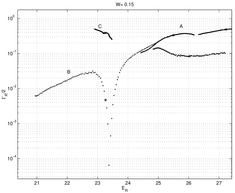
Figure 6: Eigenvalue picture: motion of the poles of the $S$-matrix in dependence on increasing length of the resonator ($y_{d}$ = -3.75 : 0.001 : -3.65). The eigenvalues at $y_{d}$ = -3.693 are marked by stars.

Two states ($B$ and $C$) cross freely in the energy at $E_{R}\approx 23$. The wavefunctions of the two states $B$ and $C$ are very different from one another and the interaction due to $\Re(W)$ between them is obviously small. The wavefunctions of both states do almost not change in the crossing region. Only in the widths, some repulsion can be seen caused obviously by $\Im(W)$. This can be seen from Figure 6 where the results are shown from a calculation with smaller steps in $y_{d}$ around the free crossing.

Around $E_{R}=27$, the state $B$ avoids crossing in energy with the other state ($A$) at some value $y_{d}^{\rm cr}$ (around -3.63). In this region, the wave functions of both states become strongly mixed, their widths become comparable and cross. The repulsion in their energies can be seen. The avoided crossing is caused mainly by $\Re(W)$. Beyond the critical region, the wavefunctions of the two states remain mixed although some hint to their exchange can be seen.

These results show that avoided level crossing in the complex plane can be seen in the projection onto the energy axis or in the projection onto the width axis. In the first case, $\Re(W)$ dominates while in the second case, the mixing of the states occurs mainly due to $\Im(W)$.

According to the oscillations of the widths and the varying number of states as a function of the length or width of the resonator, the sum of the widths of all states, lying between the two thresholds, fluctuates as a function of these values. In Figure 7 (bottom), we show the number $N$ of states as a function of $y_{d}$ (for $w=0.15$). This number increases since the number of states moving from above into the energy region considered is larger than the number of states leaving it to get bound. On the average, $\sum_{R}\Gamma_{R}$ is constant for a fixed value of $w$ with fluctuations smaller than 10 %. This can be seen from the example with $w=0.15$ shown in Figure 7 (top). The coupling of the cavity to the lead is therefore characterized by $w$ but not by the area of the cavity.

4.3 Resonances as a function of the coupling strength to the lead

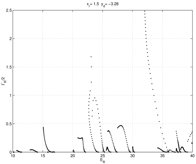
Figure 8: Eigenvalue picture: motion of the poles of the $S$-matrix in dependence on increasing opening (decreasing $w,~{}w=0.4:0.01:0)$ for $x_{r}$ = 1.5, $y_{d}$ = -3.34 (top) and $y_{d}$ = -3.28 (bottom).

In Figure 8, we show the eigenvalue picture obtained by varying $w$ from 0.4 (almost closed aperture) to 0 (fully open aperture). The width of the resonator is determined by $x_{r}=1.5$ and the length by the two neighboured values $y_{d}=-3.34$ (Figure 8 top) and $y_{d}=-3.28$ (Figure 8 bottom). In both cases, collective states are formed. They are formed in regions where the level density is comparably high. Even at full opening of the aperture, the collective states belonging to the different groups do not overlap. Thus, they scarcely mix via the continuum.

In Figure 9, we show the wavefunctions of the collective states from the lower part of Figure 8. Although the wavefunctions of the collective states are very different from one another at small opening of the aperture $(w=0.4)$, they are similar at full opening $(w=0)$ (Figures 9.d,f) where they have large amplitudes near to the aperture. The state shown in the middle (Figure 9.e) is trapped by the state to the left (Figure 9.d) at a comparably large opening (compare Figure 8 bottom). The wavefunctions of the collective states at $w=0$ in the long and in the broad resonators ($x_{r}\to 4.0,\;y_{d}\to-6.0$) are also similar to those shown in Figures 9.d and 9.f.

4.4 Resonances and conductance of the resonator

The conductance of the resonator is described by the matrix elements $S_{cc^{\prime}}$, equation (5), where $c$ is the channel of the incoming wave and $c^{\prime}$ that of the outgoing wave. In our calculations, the second lead is on the lower right corner of the cavity, symmetrically to the first lead on the upper left corner. It is $x_{r}=1.5$ and $y_{d}=-3$.

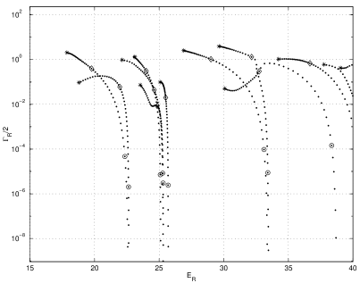
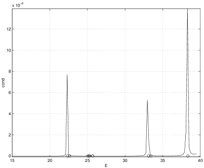
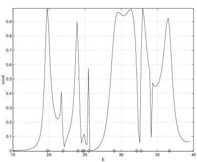
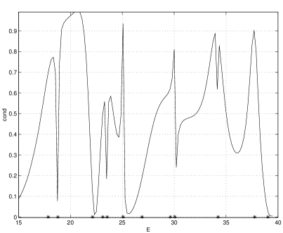
Figure 10: Eigenvalue picture: motion of the poles of the $S$-matrix in dependence on increasing opening (decreasing $w$, top left) and the conductance as a function of $E$ for $w=$ 0.4 (top right),  0.2 (bottom left) and 0 (bottom right). The values $E_{R}-(i/2)\Gamma_{R}$ and $E_{R}$, respectively, for $w=$ 0.4,  0.2 and 0 are marked by circles, diamonds and stars.

In Figure 10, the conductance at three different coupling strengths to the leads is shown together with the eigenvalue picture. In the eigenvalue picture, one can see the formation of two short-lived states at large opening (small $w$) in each group. This corresponds to the coupling of the resonator to two leads. It can be seen from the wavefunctions of the states that both short-lived states of each group are coupled strongly to both leads. The conductance is therefore large at large opening.

At low opening ($w=0.4$), the conductance peaks coincide with the resonance peaks. At larger opening ($w=0.2$ and 0), the conductance is an interference picture created by the overlapping resonances. The influence of the short-lived resonances onto the conductance can clearly be seen.

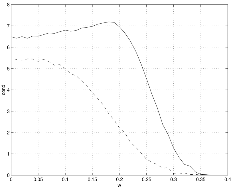
Figure 11: Integrated conductance as a function of $w$ in the energy region 25 $\leq$ E $\leq$ 40 (full line) and 15 $\leq$ E $\leq$ 25 (dashed line).

In Figure 11, the conductance is integrated over the energy of each group ($15\leq E\leq 25$ and $25\leq E\leq 40$) and plotted as a function of $w$. The conductance at the higher energy increases quite rapidly in a small region of $w$ which corresponds to the critical region around $w_{\rm cr}$ (compare [8]).

5 Discussion of the results

As demonstrated in Sections 3 and 4, the wavefunctions of a quantum system mix under the influence of the hermitian as well as the anti-hermitian part of the Hamiltonian. If the hermitian part of the Hamiltonian is dominant then avoided crossing can be seen along the energy axis (level repulsion). If the anti-hermitian part of the coupling via the continuum becomes important, then resonance trapping (bifurcation of the widths) appears. In general, both types of mixing appear and may interfere. Note that this interaction between different states of a quantum system via the continuum does not require two-body forces between the constituents of the system.

The states whose wavefunctions are shown in Figure 5 lie in the energy region around 24 where the coupling to the continuum is small. The mixing of the states is varied by means of varying the area of the resonator. In the upper part of the related Figure 4, we see typical avoided level crossings in the energies $E_{R}(y_{d})$. Here, the widths of the two states become comparable with one another. This implies that $\Re(W)$ is decisive for the process. In this case, the results are similar to those known very well from studies on closed systems with discrete states (see Section 3.1).

We see, however, also the opposite case: the crossing of the states $B$ and $C$ in Figure 4 is free along the real axis while the widths repel each other. In this case, $\Re(W)$ is obviously small (the wavefunctions of the two states are very different from one another, Figure 5). Therefore, $\Im(W)$ is decisive, and the levels can, according to Section 3.1, cross along the real axis.

The variation of the widths of the resonance states as a function of the coupling strength to the continuum is traced in Figure 8. In each group of overlapping states, one collective state is formed whose structure is determined by the channel wavefunction. This can be seen very clearly by comparing the wavefunctions of the different collective states which are similar to one another but have almost nothing in common with the original wavefunctions of these states at small opening of the aperture (Figure 9). Here, the variation of the external mixing occurs mainly in the $\Im(W)$: the approaching of the states of a group in their positions as well as the trapping of all but one state inside each group due to enlarging $\Im(W)$ can be seen very clearly in Figure 8.

It is interesting to compare Figure 8 with the results for a slightly changed geometry of the cavity. In [8], the disk is smaller and all states between the two thresholds belong to one group. According to this, only one broad state is formed at full opening of the slide.

The avoided crossing of the two broad states in the lower part of Figure 8 occurs according to the schematical picture with $iw_{\rm ex}$ (Figure 1.d, level attraction and width bifurcation) with the only difference that not only the non-diagonal matrix elements of ${\cal H}$ depend on the coupling strength determined by $w_{\rm ex}$, but also the diagonal ones. This case is studied in detail analytically and numerically in the framework of a schematical model in [11].

In [9], avoided level crossings in a closed resonator under the influence of a driving field are studied. The results show avoided level crossings with and without permanent mixing of the wavefunctions in a similar manner as in the open resonator studied by us.

The relation between the peaks in the conductance, the Wigner delay times and the positions of the states in the closed resonator is studied in [18]. The results of the present paper show that the conductance peaks are related to the positions of the resonance states in the open resonator. The peaks are, generally, the result of interferences between the resonance states.

Altogether, the interplay between $\Re(W)$ and $\Im(W)$ leads, as a rule, to permanent mixings of the wavefunctions. Level repulsion along the real axis is caused by $\Re(W)$ while bifurcation of the widths (resonance trapping) is caused by $\Im(W)$. Both processes may interfere. As a result, different time scales may appear and the energy dependency of the conductance changes with the degree of opening of the system in a non-trivial manner.

6 Conclusions

The interaction $W$ of resonance states via the continuum of decay channels consists of the hermitian part $\Re(W)$ and the anti-hermitian part $\Im(W)$. Both terms have to be considered not only in a many-body system [10] but also in the micro-wave billiard as shown in the present paper. Some results show the dominance of $\Im(W)$, others the dominance of $\Re(W)$. The avoided crossing of the resonance states in the complex plane may appear, under certain conditions, as a free crossing along the real axis or along the imaginary axis.

The interplay between the hermitian and anti-hermitian parts of the coupling operator between two resonance states via a common continuum may lead, in some cases, to a bifurcation of the widths (resonance trapping). In other cases, it may lead to a repulsion of the states along the real energy axis. The interaction $W$ introduces, as a rule, permanent changes in the wavefunctions of the resonance states. Under certain conditions, the system may be stabilized dynamically [3].

The resonance picture of a microwave resonator shows all the characteristic features which are known from open quantum systems with two-body forces between the constituents. This result means that the interaction between the resonance states at the avoided level crossings in the complex plane plays an important role for the mixing of the wavefunctions. As an example, the wavefunctions of the collective short-lived states are strongly mixed in the set of wavefunctions of the closed system. They are quite different from those of the original states at small coupling to the continuum.

The statistical theory (random matrix theory) describes resonance states of an almost closed system. The poles of the $S$-matrix are near to the real axis and $\Im(W)$ is small. The effective Hamilton operator is ${\cal H}={\cal H}_{0}+\Re(W)+\Im(W)=\Re({\cal H})-iVV^{\dagger}$ where the $V$ are the coupling vectors between discrete and scattering states [19]. The level repulsion along the real energy axis is embodied in $\Re({\cal H})$ by choosing, e.g., the Gaussian orthogonal ensemble. Under these conditions, the effects caused by the interplay between $\Re({\cal H})$ and $\Im({\cal H})$ can be neglected to a good approximation. The results obtained in the present paper show, however, that the situation is different when the system is really open, i.e. when $\Im({\cal H})$ and $\Re({\cal H})$ are of the same order of magnitude. In this case, the interplay between the two parts of ${\cal H}$ causes non-negligible effects which are not considered in the statistical theory. The avoided crossing of resonance states in the complex plane embodies the interplay between resonance trapping and level repulsion along the real axis.

Acknowledgment: Valuable discussions with J. Burgdörfer, M. Müller, J. Nöckel, K. Richter and M. Sieber are gratefully acknowledged.

Figure 1: Eigenvalue picture: motion of the poles of the $S$-matrix in dependence on increasing $v_{\rm in}$ (a) and $w_{\rm ex}$ (d). The mixing of the wavefunctions in dependence on $v_{\rm in}$ (b,c) and $w_{\rm ex}$ (e,f). At $v_{\rm in}=0$ and $w_{\rm ex}=0$, respectively, $b_{ij}=\delta(i,j)$ (marked by arrows).

Figure 5: The wavefunctions of the 3 states A (left), B (middle) and C (right) shown in Figure 4 for $x_{r}$ = 1.5 and $y_{d}$ = -3.56 (1), -3.58 (2) -3.60 (3), -3.62 (4), -3.64 (5), -3.66 (6), -3.68 (7), -3.70 (8), -3.72 (9), -3.74 (10).

Figure 7: The sum $\sum_{R}\Gamma_{R}$ of the widths (top) and the number $N$ (bottom) of the states lying between the two thresholds shown as a function of the length $y_{d}$ of the cavity. $w=0.15$.

Figure 9: The wavefunctions of the 3 broad states shown in the lower part of Figure 8 at $w$ = 0.4 (a, b, c) and $w$ = 0 (d, e, f). The state in the middle (b, e) becomes trapped by the state to the left (a, d).

References

- [1] V.V. Sokolov and V. Zelevinsky, Phys. Rev. C 56, 311 (1997); E. Persson and I. Rotter, Phys. Rev. C 59, 164 (1999)
- [2] V.V. Sokolov, I. Rotter, D.V. Savin and M. Müller, Phys. Rev. C 56, 1031 and 1044 (1997)
- [3] A.I. Magunov, I. Rotter and S.I. Strakhova, J. Phys. B 32, 1489 and 1669 (1999)
- [4] M. Desouter-Lecomte and J. Liévin, J. Chem. Phys. 107, 1428 (1997); I. Rotter, J. Chem. Phys. 106, 4810 (1997); M. Desouter-Lecomte and X. Chapuisat, Physical Chemistry Chemical Physics 1, 2635 (1999)
- [5] Y.V. Fyodorov and H.J. Sommers, J. Math. Phys. 38, 1918 (1997); T. Gorin, F.M. Dittes, M. Müller, I. Rotter and T.H. Seligman, Phys. Rev. E 56, 2481 (1997); E. Persson, T. Gorin and I. Rotter, Phys. Rev. E 58, 1334 (1998); C. Jung, M. Müller and I. Rotter, Phys. Rev. E 60, 114 (1999)
- [6] W.D. Heiss, M. Müller, and I. Rotter, Phys. Rev. E 58, 2894 (1998)
- [7] E. Persson, K. Pichugin, I. Rotter and P. eba, Phys. Rev. E 58, 8001 (1998)
- [8] P. eba, I. Rotter, M. Müller, E. Persson and K. Pichugin, Phys. Rev. E 61, 66 (2000)
- [9] T. Timberlake and L.E. Reichl, Phys. Rev. A 59, 2886 (1999)
- [10] S. Drożdż, J. Okołowicz, M. Płoszajczak and I. Rotter, nucl-th/9912055
- [11] M. Müller, F.M. Dittes, W. Iskra and I. Rotter, Phys. Rev. E 52 5961 (1995)
- [12] I. Rotter, Rep. Progr. Phys. 54, 635 (1991) and to be published
- [13] R.G. Newton, Scattering Theory of Waves and Particles, Springer, New York 1982
- [14] P. von Brentano and M. Philipp, Phys. Lett. B 454, 171 (1999) and references therein
- [15] U. Fano, Phys. Rev. 124, 1866 (1961)
- [16] B. Simon, Int. J. Quant. Chem. 14, 529 (1978)
- [17] A. Jensen, J. Math. Anal. Appl. 59, 505 (1977)
- [18] S. Ree and L.E. Reichl, Phys. Rev. B 59, 8163 (1999)
- [19] C. Mahaux and H.A. Weidenmüller, Shell model approach to nuclear reactions, North-Holland, Amsterdam, 1969