On Fine’s resolution of the EPR-Bell problem

• László E. Szabó

• $\overline{\,\,\,\,\,\,\,\,\,\,\,\,\,\,\,\,\,\,\,\,\,\,\,\,\,\,\,\,\,\,\,\,\,\,\,\,\,\,\,\,\,\,\,\,\,\,\,\,\,\,\,\,\,\,\,\,\,\,\,\,\,\,\,\,\,\,\,\,\,\,\,\,\,\,\,\,\,\,\,\,\,\,\,\,\,\,\,\,\,\,\,\,\,\,\,\,\,\,\,\,\,\,\,\,\,\,\,\,\,\,\,\,\,\,\,\,\,\,\,\,\,\,\,\,\,\,\,\,\,\,\,\,\,\,\,\,\,\,\,\,\,\,\,\,\,\,\,\,\,\,\,\,\,\,\,\,\,\,\,\,\,\,\,\,\,\,\,\,\,\,\,\,\,\,\,\,}$
  In the real spin-correlation experiments the detection/emission inefficiency is usually ascribed to independent random detection errors, and treated by the “enhancement hypothesis”. In Fine’s “prism model” the detection inefficiency is an effect not only of the random errors in the analyzer + detector equipment, but is also the manifestation of a pre-settled (hidden) property of the particles.
  $\underline{\,\,\,\,\,\,\,\,\,\,\,\,\,\,\,\,\,\,\,\,\,\,\,\,\,\,\,\,\,\,\,\,\,\,\,\,\,\,\,\,\,\,\,\,\,\,\,\,\,\,\,\,\,\,\,\,\,\,\,\,\,\,\,\,\,\,\,\,\,\,\,\,\,\,\,\,\,\,\,\,\,\,\,\,\,\,\,\,\,\,\,\,\,\,\,\,\,\,\,\,\,\,\,\,\,\,\,\,\,\,\,\,\,\,\,\,\,\,\,\,\,\,\,\,\,\,\,\,\,\,\,\,\,\,\,\,\,\,\,\,\,\,\,\,\,\,\,\,\,\,\,\,\,\,\,\,\,\,\,\,\,\,\,\,\,\,\,\,\,\,\,\,\,\,\,\,}$

1 Introduction

The aim of this paper is to make an introduction to Fine’s interpretation of quantum mechanics and to show how it can solve the EPR–Bell problem. In the real spin correlation experiments the measured quantum probabilities are identified with relative frequencies taken on a selected sub-ensemble of the emitted particle pairs: only those particles are taken into account which are coincidentally detected in the two wings. The detection/emission inefficiency is usually ascribed to random detection errors occurring independently in the two wings, and treated by the “enhancement hypothesis”, which assumes that the relative frequencies measured on the randomly selected sub-ensemble are equal to the ones taken on the whole statistical ensemble of emitted particle pairs.

Fine’s prism model⁽¹⁾ is a local hidden variable theory, in which the detection inefficiency is an effect not only of the random errors in the analyzer + detector equipment, but is also the manifestation of a predetermined hidden property of the particles. I present one of Fine’s prism models for the EPR experiment and compare it with the recent experimental results.⁽²⁾ As we shall see, it works well in case of the $2\times 2$ spin-correlation experiments. There appeared, however, a theoretical demand to embed the $2\times 2$ prism models into a large $n\times n$ prism model reproducing all potential $2\times 2$ sub-experiments. This demand was motivated by the idea that the real physical process does not know which directions are chosen in an experiment. On the other hand, it seemed that in the known prism models of the $n\times n$ spin-correlation experiment the efficiencies tended to zero, if $n\rightarrow\infty~{}$, which contradicts what we expect of actual experiments.⁽³⁾ This problem is investigated in the last part of the paper.

2 Real EPR experiments

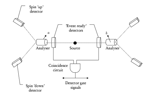
Figure 1: Apparatus configuration used for Bell’s 1971 proof. ‘Event-ready’ detectors signal both arms that a pair of particles has been emitted

Figure 1 shows an Aspect-type spin-correlation experiment. The analyzers can be set in orientation $a$ or $a^{\prime}$ on the left hand side, and $b$ or $b^{\prime}$ on the right. Denote $A$, $A^{\prime}$, $B$ and $B^{\prime}$ the corresponding “spin-up” detection-events. $p(A|a)$, for instance, denotes the conditional probability of $A$, given that the measurement set-up in the left wing is $a$.

Now, from the assumption that there exists a hidden variable $\lambda$ satisfying the screening off condition,

$$p\left(A\wedge B|a\wedge b\wedge\lambda\right)=p\left(A|a\wedge\lambda\right)p\left(B|b\wedge\lambda\right)$$

one can derive⁽⁴⁾ the well known Clauser-Horne inequality:

$$-1\leq\underbrace{\left\{\begin{array}[]{c}p\left(A\wedge B|a\wedge b\right)+p\left(A\wedge B^{\prime}|a\wedge b^{\prime}\right)-p\left(A^{\prime}\wedge B|a^{\prime}\wedge b\right)\\ +p\left(A^{\prime}\wedge B^{\prime}|a^{\prime}\wedge b^{\prime}\right)-p\left(A^{\prime}|a^{\prime}\right)-p\left(B|b\right)\end{array}\right\}}_{CH}\leq 0$$ (1)

According to the standard views, inequality (1) is violated in the real spin-correlation experiments, hence, the argument goes, any local hidden variable theory for the EPR experiment is excluded. For example, in case of spin-$\frac{1}{2}$ particles, if the directions $a$, $a^{\prime}$, $b$, $b^{\prime}$ are coplanar with $\angle(a,b)=\angle(a,b^{\prime})=\angle(a^{\prime},b^{\prime})=120^{\circ}$ and $\angle(a^{\prime},b)=0$, then the Clauser-Horne expression in (1) is

$$CH=\frac{3}{8}+\frac{3}{8}-0+\frac{3}{8}-\frac{1}{2}-\frac{1}{2}=\frac{3}{8}$$ (2)

There is, however a serious loophole in the real experiments. Compare the original apparatus configuration used for Bell’s 1971 proof with the one used in the real Aspect experiment (Fig. 1 and 2). The original configuration contains two ‘event-ready’ detectors, which signal both arms that a pair of particles has been emitted. So, the statistics are taken on the ensemble of particle pairs emitted by the source. In the real experiments, however, instead of the event-ready detectors, a four-coincidence circuit detects the ‘emitted particle-pairs’. This method yields to a selected statistical ensemble: only those pairs are taken into account, which coincidentally fire one of the left and one of the right detectors. Denote $\left[A\right]$ the event that there is any detection in the left wing with analyzer set-up $a$, that is, either the “up” detector or the “down” detector fires. Similarly, $\left[A\right]\wedge\left[B\right]$ denotes the corresponding double detection. So, what we actually observe is the violation of the following inequality:

$$-1\leq\left\{\begin{array}[]{c}p\left(A\wedge B|a\wedge b\wedge\left[A\right]\wedge\left[B\right]\right)+p\left(A\wedge B^{\prime}|a\wedge b^{\prime}\wedge\left[A\right]\wedge\left[B^{\prime}\right]\right)\\ -p\left(A^{\prime}\wedge B|a^{\prime}\wedge b\wedge\left[A^{\prime}\right]\wedge\left[B\right]\right)+p\left(A^{\prime}\wedge B^{\prime}|a^{\prime}\wedge b^{\prime}\wedge\left[A^{\prime}\right]\wedge\left[B^{\prime}\right]\right)\\ -p\left(A^{\prime}|a^{\prime}\wedge\left[A^{\prime}\right]\right)-p\left(B|b\wedge\left[B\right]\right)\end{array}\right\}\leq 0$$ (3)

If the selection procedure were completely random then the observed relative frequencies on the selected ensemble would be equal to the ones taken on the original ensemble, that is,

$$p\left(A\wedge B|a\wedge b\wedge\left[A\right]\wedge\left[B\right]\right) = p\left(A\wedge B|a\wedge b\right)$$

$$p\left(A\wedge B^{\prime}|a\wedge b^{\prime}\wedge\left[A\right]\wedge\left[B^{\prime}\right]\right) = p\left(A\wedge B^{\prime}|a\wedge b^{\prime}\right)$$

$$\textrm{etc}.$$

(enhancement hypothesis) and the violation of inequality (3) would imply the violation of (1), in accordance with Bell’s point of view:

… it is hard for me to believe that quantum mechanics works so nicely for inefficient practical set-ups and is yet going to fail badly when sufficient refinements are made. (Ref. 5, p. 154)

This is indeed the case if non-detections are caused by independent random errors in the detector+analyser equipment.

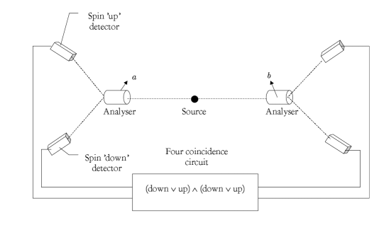
Figure 2: In the real experiments, instead of the event-ready detectors, a four-coincidence circuit detects the ‘emitted particle-pairs’

3 Fine’s interpretation

Arthur Fine approaches the detection inefficiency problem in a different way:

… the efficiency problem ought not to be dismissed as merely one of biased statistics and conspiracies, for the issue it raises is fundamental. Can a hidden variable theory of the very type being tested explain the statistical distributions, inefficiencies and all, actually found in the experiments? If so then we would have a model (or theory) of the experiment that explains why the samples counted yield the particular statistics that they do. (Ref. 6, p. 465)

This conception of hidden variable was first realized in Fine’s prism models⁽¹⁾ for the $2\times 2$ spin-correlation experiment. Prism model is a local, deterministic hidden variable theory, in which the hidden variables predetermine not only the outcomes of the corresponding measurements, but also predetermine whether or not an emitted particle arrives to the detector and becomes detected. In other words, the measured observables can take on a new “value” corresponding to an inherent “no show” or defectiveness.

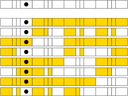
Figure 3: Parameter $\lambda\in\Lambda$ completely predetermines all future events for all possible combinations of the freely chosen measurements. Each EPR event is represented as a (shaded) subset of $\Lambda$.

As an example, consider a prism model reproducing the quantum mechanical probabilities in (2). Figure 3 shows a parameter space $\Lambda\ni\lambda$ consisting of disjoint blocks of measure $\frac{3}{32}$ and $\frac{1}{32}$ respectively. A point of $\Lambda$ (a value of the parameter $\lambda$) predetermines all events in question. Therefore, each EPR event can be represented as a subset of $\Lambda$. For instance, assume that $\lambda=\lambda_{\mathrm{example}}$. Then, an $a$-measurement on the left particle produces neither event “up” nor event “down”, while if an $a^{\prime}$-measurement is performed then the outcome is “down”. In the right wing, if we perform a $b$-measurement then the outcome is “up”, and if the $b^{\prime}$-measurement is performed, the outcome is “down”. Consequently, in case, for example, we perform an $a$-measurement on the left particle and a $b$-measurement on the right one, then there is no coincidence registered, and the particle pair in question does not appear in the statistics of the measurement. On the contrary, if we perform an $a^{\prime}$-measurement on the left particle and a $b$-measurement on the right one, then there is a coincidence registered and the counter of the total number of events as well as the $B$-counter count. Thus, the hidden parameter governs the whole process in such a way that the observed relative frequencies reproduce the probabilities measured in the experiment:

$$\frac{\mu\left(A\right)}{\mu\left([A]\right)} = \frac{\mu\left(A^{\prime}\right)}{\mu\left([A^{\prime}]\right)}=\frac{\mu\left(B\right)}{\mu\left([B]\right)}=\frac{\mu\left(B^{\prime}\right)}{\mu\left([B^{\prime}]\right)}=\frac{\frac{12}{32}}{\frac{24}{32}}=\frac{1}{2}$$

$$\frac{\mu\left(A\cap B\right)}{\mu\left([A]\cap[B]\right)} = \frac{\mu\left(A\cap B^{\prime}\right)}{\mu\left([A]\cap[B^{\prime}]\right)}=\frac{\mu\left(A^{\prime}\cap B^{\prime}\right)}{\mu\left([A^{\prime}]\cap[B^{\prime}]\right)}=\frac{\frac{6}{32}}{\frac{16}{32}}=\frac{3}{8}$$

$$\frac{\mu\left(A^{\prime}\cap B\right)}{\mu\left([A^{\prime}]\cap[B]\right)} = \frac{0}{\frac{16}{32}}=0$$

4 Compatibility with the actual EPR experiments

As we have seen, the basic idea of the Einstein–Fine interpretation is that some elements of the statistical ensemble of identically prepared quantum systems (characterized by a quantum state $W$) do not produce outcome at all when one perform the measurement of a quantum observable $A$. Such systems are called $A$-defective in Fine’s terminology. In connection with this basic feature of the model, one can investigate some important characteristics of the above Einstein–Fine model of the EPR experiment, and compare them with the similar characteristics of the actual EPR experiments:

$$R^{A} = \frac{\textrm{number of non}-A-\textrm{defective systems}}{\textrm{total number of systems}}$$

$$R^{A^{\prime}} = \frac{\textrm{number of non}-A^{\prime}-\textrm{defective systems}}{\textrm{total number of systems}}$$

$$R^{B} = \frac{\textrm{number of non}-B-\textrm{defective systems}}{\textrm{total number of systems}}$$

$$R^{B^{\prime}} = \frac{\textrm{number of non}-B^{\prime}-\textrm{defective systems}}{\textrm{total number of systems}}$$

$$R^{AB} = \frac{\textrm{number of non}-A-\textrm{defective }\&\textrm{ non}-B-\textrm{defective systems}}{\textrm{total number of systems}}$$

$$R^{AB^{\prime}} = \frac{\textrm{number of non}-A-\textrm{defective }\&\textrm{ non}-B^{\prime}-\textrm{defective systems}}{\textrm{total number of systems}}$$

$$R^{A^{\prime}B} = \frac{\textrm{number of non}-A^{\prime}-\textrm{defective }\&\textrm{ non}-B-\textrm{defective systems}}{\textrm{total number of systems}}$$

$$R^{A^{\prime}B^{\prime}} = \frac{\textrm{number of non}-A^{\prime}-\textrm{defective }\&\textrm{ non}-B^{\prime}-\textrm{defective systems}}{\textrm{total number of systems}}$$

In case of the above example:

$$\begin{array}[]{rcl}R^{A}=R^{A^{\prime}}=R^{B}=R^{B^{\prime}}&=&75\%\\ R^{AB}=R^{AB^{\prime}}=R^{A^{\prime}B}=R^{A^{\prime}B^{\prime}}&=&50\%\end{array}$$ (4)

If any of the similar rates in a real experiment were higher than the corresponding one in (4), Fine’s interpretation would be experimentally refuted.

There are principal obstacles to an event ready detection, therefore we cannot have a precise information about the total number of systems. In one of the best experiments of the last years⁽²⁾ the estimated rates are the following:

$$\begin{array}[]{rcl}R^{A}=R^{A^{\prime}}=R^{B}=R^{B^{\prime}}&=&5\%\\ R^{AB}=R^{AB^{\prime}}=R^{A^{\prime}B}=R^{A^{\prime}B^{\prime}}&=&0.25\%\end{array}$$ (5)

So the prism model is in accordance with this experiment.

It can be (and probably is) the case that this very low detection/emission rate is mostly caused by the external random detection errors, different from the prism mechanism. In order to separate these two sources of inefficiency, consider a new characteristic of the model:

$$r_{A}^{AB}=\frac{\textrm{number of non}-A-\textrm{defective }\&\textrm{ non}-B-\textrm{defective systems}}{\textrm{number of non}-A-\textrm{defective systems}}$$

$$r_{A}^{AB^{\prime}}=\frac{\textrm{number of non}-A-\textrm{defective }\&\textrm{ non}-B^{\prime}-\textrm{defective systems}}{\textrm{number of non}-A-\textrm{defective systems}}$$

$$\vdots$$ (6)

$$r_{B^{\prime}}^{A^{\prime}B^{\prime}}=\frac{\textrm{number of non}-A^{\prime}-\textrm{defective }\&\textrm{ non}-B^{\prime}-\textrm{defective systems}}{\textrm{number of non}-B^{\prime}-\textrm{defective systems}}$$

In our prism model:

$$r_{A}^{AB}=r_{A}^{AB^{\prime}}=r_{A^{\prime}}^{A^{\prime}B}=r_{A^{\prime}}^{A^{\prime}B^{\prime}}=r_{B}^{AB}=r_{B^{\prime}}^{AB^{\prime}}=r_{B}^{A^{\prime}B}=r_{B^{\prime}}^{A^{\prime}B^{\prime}}=66,66\%$$

The experiment by Weihs et al.⁽²⁾ had a particular new feature: In the two wings independent data registration was performed by each observer having his own atomic clock, synchronized only once before each experiment cycle. A time tag was stored for each detected photon in two separate computers at the observer stations and the stored data were analyzed for coincidences long after measurements were finished. Due to this method of data registration, it was possible to count the rates in (6). Again, if any of these rates were higher than 66,66%, Fine’s interpretation wouldn’t be tenable. However the experimental values were only around 5%.

5 The prism model of an $n\times n$ spin correlation experiment

Let us turn now to a serious objection to Fine’s approach. In the EPR experiment we consider only $2\times 2$ different possible directions ($\overrightarrow{a},\overrightarrow{a}^{\prime},\overrightarrow{b},\overrightarrow{b}^{\prime}$). If nature works according to Fine’s prism model then there must exist, in principle, a larger $n\times n$ prism model reproducing all potential $2\times 2$ sub-experiments. It is because nature does not know about how the experiment is designed. So, in the final analysis, there is no such a thing as $2\times 2$ prism model of the $2\times 2$ spin-correlation experiment. If we want to describe a $2\times 2$ spin-correlation experiment with a prism model, then there must exist a large $n\times n$ (if not $\infty\times\infty)$ prism model behind it.

The general schema of the prism model of a spin-correlation experiment is the following. In both wings one considers $n$ different possible events:

$$\overbrace{\underbrace{A_{1},A_{2}}_{\left[A_{1}\right]=\left[A_{2}\right]},\underbrace{A_{3},A_{4}}_{\left[A_{3}\right]=\left[A_{4}\right]},\ldots\underbrace{A_{n-1},A_{n}}_{\left[A_{n-1}\right]=\left[A_{n}\right]}}^{\mathrm{left}}\,\,\,\,\,\overbrace{\underbrace{B_{1},B_{2}}_{\left[B_{1}\right]=\left[B_{2}\right]},\underbrace{B_{3},B_{4}}_{\left[B_{3}\right]=\left[B_{4}\right]},\ldots\underbrace{B_{n-1},B_{n}}_{\left[B_{n-1}\right]=\left[B_{n}\right]}}^{\mathrm{right}}$$ (7)

$A_{1}$ denotes the event that the left particle has spin “up” along direction $\overrightarrow{a}_{1}$. $A_{2}$ denotes the event that the left particle has spin “down” along direction $\overrightarrow{a}_{1}$. Similarly, $A_{3}$ denotes the event that the left particle has spin “up” along direction $\overrightarrow{a}_{3}$ and $A_{4}$ denotes the event that the left particle has spin “down” along direction $\overrightarrow{a}_{3}$, etc. (We will also use the following notation: $\overrightarrow{a}_{2}=\overrightarrow{a}_{1},\overrightarrow{a}_{4}=\overrightarrow{a}_{3},\dots\overrightarrow{a}_{2k}=\overrightarrow{a}_{2k-1},\dots\overrightarrow{b}_{2k}=\overrightarrow{b}_{2k-1}$.) There are $\frac{n}{2}$ different directions on both sides. We also assume the following logical relationships:

$$\begin{array}[]{rcllrcl}\left[A_{1}\right]=\left[A_{2}\right]&=&A_{1}\vee A_{2}&&\left[B_{1}\right]=\left[B_{2}\right]&=&B_{1}\vee B_{2}\\ \left[A_{3}\right]=\left[A_{4}\right]&=&A_{3}\vee A_{4}&&\left[B_{3}\right]=\left[B_{4}\right]&=&B_{3}\vee B_{4}\\ &\vdots&&&&\vdots&\\ \left[A_{n-1}\right]=\left[A_{n}\right]&=&A_{n-1}\vee A_{n}&&\left[B_{n-1}\right]=\left[B_{n}\right]&=&B_{n-1}\vee B_{n}\\ A_{1}\wedge A_{2}&=&0&&B_{1}\wedge B_{2}&=&0\\ A_{3}\wedge A_{4}&=&0&&B_{3}\wedge B_{4}&=&0\\ &\vdots&&&&\vdots&\\ A_{n-1}\wedge A_{n}&=&0&&B_{n-1}\wedge B_{n}&=&0\end{array}$$ (8)

that is, $\left[A_{1}\right]$ (which is equal to $\left[A_{2}\right]$) denotes the event that the left particle is predetermined to produce any outcome if the $\overrightarrow{a}_{1}$ direction is measured. The quantum probabilities are reproduced in the following way:

$$tr\left(WP_{A_{i}}\right)=q_{i} = \frac{p\left(A_{i}\right)}{p\left(\left[A_{i}\right]\right)}$$

$$tr\left(WP_{B_{i}}\right)=q^{\prime}_{i} = \frac{p\left(B_{i}\right)}{p\left(\left[B_{i}\right]\right)}$$ (9)

$$tr\left(WP_{A_{i}}P_{B_{j}}\right)=q_{ij} = \frac{p\left(A_{i}\wedge B_{j}\right)}{p\left(\left[A_{i}\right]\wedge\left[B_{j}\right]\right)}$$

The quantum probabilities $q_{1},q_{2},\ldots q^{\prime}_{1},q^{\prime}_{2},\ldots q_{ij},\ldots$ are the only fix numbers in the model.

The experimental setup shows the following simple and natural symmetries:

• None of the left and right wings is privileged.

• There is no privileged direction among the possible polariser positions.

Consequently, all physically plausible prism model have to satisfy these symmetry conditions, which imply the following two constraints:

$$p\left(\left[A_{i}\right]\right)=\omega\quad\quad\textrm{for all }1\leq i\leq n$$ (10)

where $\omega$ is some uniform efficiency for all directions on both sides, and

$$p\left(\left[A_{i}\right]\wedge\left[B_{j}\right]\right)=\sigma\left(\angle\left(\overrightarrow{a}_{i},\overrightarrow{b}_{j}\right)\right)\quad\quad\textrm{for all }1\leq i,j\leq n$$ (11)

where $0\leq\sigma\left(\angle\left(\overrightarrow{a}_{i},\overrightarrow{b}_{j}\right)\right)\leq\omega$ is an arbitrary function of the angel $\angle\left(\overrightarrow{a}_{i},\overrightarrow{b}_{j}\right)$.

Thus, the prism-model resolution of the EPR-Bell problem requires the existence of $n\times n$ prism models of the above type. On the other hand, this requirement appears to be a serious objection to Fine’s program. The reason is that in all the known $n\times n$ prism models the efficiency $\omega$ tends to zero if $n\rightarrow\infty$, which contradicts the recent experimental results.^(7-8) Moreover, Fine has shown⁽³⁾ that this is true for the class of $n\times n$ prism models satisfying certain symmetry conditions called Exchangeability, Indifference and Strong Symmetry. They are complex conditions, too complex to briefly recall the definitions. Although they do not express some natural and obvious symmetries of the experimental setup, they are instanced in all the known prism models.

If all physically plausible prism models had to satisfy the Exchangeability, Indifference and Strong Symmetry conditions, the problem of zero efficiency would mean a serious objection to Fine’s interpretation. Fortunately, this is not the case. In my http://arXiv.org/abs/quant-ph/0012042 I shown the existence of $\infty\times\infty$ prism models satisfying the symmetry conditions (S1) and (S2), whereas the efficiencies are reasonably high.

References

1. A. Fine, “Some local models for correlation experiments”, Synthese, 50, 279 (1982)

2. G. Weihs, T. Jennewin, C. Simon, H. Weinfurter, and A. Zeilinger, “Violation of Bell’s Inequality under Strict Einstein Locality Conditions”, Phys. Rev. Lett., 81, 5039 (1998)

3. A. Fine, “Inequalities for Nonideal Correlation Experiments”, Foundations of Physics, 21, 365 (1991)

4. B. C. van Frassen, “The Charybdis of Realism: Epistemological Implications of Bell’s Inequality”, in Philosophical Consequences of Quantum Theory – Reflections on Bell’s Theorem, J. T. Cushing and E. McMullin (eds.), University of Notre Dame Press, Notre Dame, (1989)

5. J. S. Bell, Speakable and unspeakable in quantum mechanics, Cambridge University Press, Cambridge, (1987)

6. A. Fine, “Correlations and Efficiency: Testing Bell Inequalities”, Foundations of Physics, 19, 453 (1989)

7. W. D. Sharp and N. Shank, , “Fine’s prism models for quantum correlation statistics”, Philosophy of Science, 52, 538 (1985)

8. T. Maudlin, Quantum Non-Locality and Relativity – Metaphysical Intimations of Modern Physics, Aristotelian Society Series, Vol. 13, Blackwell, Oxford, (1994)