Abstract

We show that in the dissipative quantum model of brain the time-dependence of the frequencies of the electrical dipole wave quanta leads to the dynamical organization of the memories in space (i.e. to their localization in more or less diffused regions of the brain) and in time (i.e. to their longer or shorter life-time). The life-time and the localization in domains of the memory states also depend on internal parameters and on the number of links that the brain establishes with the external world. These results agree with the physiological observations of the dynamic formation of neural circuitry which grows as brain develops and relates to external world.

*This paper is dedicated to Professor Karl H. Pribram in the occasion of his 80th birthday.

1 Introduction

Since Lashely’s experimental work in the forties it has been known that many functional activities of the brain cannot be directly related to specific neural cells, rather they involve extended regions of the brain. In Lashely’s words, as reported by Pribram[1], ”all behaviour seems to be determined by masses of excitation, by the form or relations or proportions of excitation within general fields of activity, without regard to particular nerve cells”. Pribram’s subsequent work, confirming and extending Lashely observations, brought him in the sixties to introduce concepts of Quantum Optics, such as holography, in brain modeling[1, 2]. The description of non-locality of brain functions, especially of memory storing and recalling, also was the main goal of the quantum brain model proposed in the 1967 by Ricciardi and Umezawa[3]. This model is based on the Quantum Field Theory (QFT) of many body systems and its main ingredient is the mechanism of spontaneous breakdown of symmetry. In recent years, the Ricciardi and Umezawa quantum model, further developed by Stuart, Takahashi and Umezawa[4, 5] (see also [6]), has attracted much interest since it exhibits interesting features also related with the rôle of microtubules in the brain activity[1, 2, 7]. It has been shown that in the quantum brain model an essential rôle is played by the electrical dipole vibrational modes, from now on named dipole wave quanta (dwq), of the water molecules and of other biomolecules present in the brain structures[7]. Moreover, the extension of the model to dissipative dynamics has revealed to be crucial in order to allow a huge memory capacity[8]. The dissipative quantum model of brain has been recently investigated[9] also in relation with the possibility of modeling neural networks exhibiting collective dynamics and long range correlations among the net units. The study of quantum dynamical features for neural nets is of course of great interest either in connection with computational neuroscience, either in connection with quantum computational strategies based on quantum evolution (quantum computation)[10].

In ref. [8] it has been considered the case of time independent frequencies associated to the dwq. A more general case is the one of time-dependent frequencies. The dwq may in fact undergo a number of fluctuating interactions and then their characteristic frequency may accordingly change in time. The aim of this paper is to show that dissipativity and frequency time-dependence lead to the dynamical organization of the memories in space (i.e. to their localization in more or less diffused regions of the brain) and in time (i.e. to their longer or shorter life-time).

The results we obtain appear to agree with physiological observations which show that many functions related to external world, such as movement, memory, vision, cannot be attributed to specific brain cells or structures, rather they involve different assembly of neurons in a way to ”generate a connected whole”[11]. The neural connectivity is observed to grow as the brain develops and relates to the external world. In previous studies of the quantum brain model the region involved in memory recording (and recalling) was extending to the full system. According to the results below presented, we have now ”domains” of finite size involved in certain functions (essentially memory related functions). As observed in ref. [8], the finiteness of the size of the domains implies an effective non-zero mass for the dwq (which, on the contrary, are massless in the case of the infinite volume system) and this in turn implies the appearance of related time-scales for the dwq propagation inside the domain. The arising of these time-scales seems to match physiological observation of time lapses observed in gradual recruitment of neurons in the establishment of brain functions[11]. On the other hand, frequency time-dependence also introduces a fine structure in the decay behavior of memories, which adds up to the memory decay features implied by dissipativity (see ref. [8]).

The paper is organized as follows. In Sec. 2, for the reader convenience, we present a summary of the main features of the dissipative quantum brain model. In Sec. 3 we show that such a couple of equations may actually be derived from the spherical Bessel equation of given order, say $n$, when the frequency is (exponentially) time-dependent. We will see that the order $n$ provides a measure of the ”openness” of the brain over the external world, i.e. of the number of links (couplings) that the brain can establish with the environment. In Sec. 4 we consider the emergence of finite life-times for the memories and relate them to the sizes of the corresponding domains in the brain. Sec. 5 is devoted to further remarks and to conclusions. Finally, some details of the mathematical formalism are reported in the Appendix.

2 The dissipative quantum brain model

As it is well known, in quantum field theory (QFT) the spontaneous breakdown of symmetry occurs when the Lagrangian is invariant under certain group of continuous symmetry, say $G$, and the vacuum or ground state of the system is not invariant under $G$, but under one of its subgroups, say $G^{\prime}$. In such a case, the ground state exhibits observable ordered patterns, specific of the breakdown of $G$ into $G^{\prime}$. It can be shown [12, 13] that these observable ordered patterns are generated by the coherent condensation in the ground state of massless quasiparticles called Nambu-Goldstone (NG) modes. These are thus the carriers of the ordering information in the ground state or vacuum. Their range of propagation covers the full system and therefore they manifest themselves as collective modes (we are assuming to be in the infinite volume limit as required by QFT). The observable specifying the degree of ordering of the vacuum (called the order parameter) acts as a macroscopic variable for the system and is specific of the kind of symmetry into play. Its value is related with the density of condensed NG bosons in the vacuum. Such a value may thus be considered as the code specifying the vacuum of the system (i.e. its physical phase) among many possible degenerate vacua.

In the quantum model of brain[3]-[7] the information storage function, i.e. memory recording, is represented by the ”coding” of (i.e. the ordering induced in) the ground state by means of the condensation of NG modes due to the breakdown of the rotational symmetry of the electrical dipoles of the water molecules. The corresponding NG mode are the vibrational dipole wave quanta (dwq) (in analogy to what happens in the QFT modeling of living matter[14]). The trigger of the symmetry breakdown is the external informational input. It has been shown[8] that by taking into account the intrinsic dissipative character of the brain dynamics, namely that the brain is an open system continuously linked (coupled) with the environment, the memory capacity can be enormously enlarged, thus solving one of the main problems left unsolved in the original formulation of the quantum brain model.

The procedure of the canonical quantization of a dissipative system requires[8, 15] the ”doubling” of the degrees of freedom of the system. Let $A_{\kappa}$ and ${\tilde{A}}_{\kappa}$ denote the dwq mode and its ”doubled mode”, respectively. The suffix $\kappa$ denotes the momentum. In general there could be other suffices denoting other degrees of freedom of the modes $A$ and $\tilde{A}$. The $\tilde{A}$ mode is the ”time-reversed image”, i.e. the ”mirror in time image” of the $A$ mode and it represents the environment mode. Quantum field modes are associated with oscillator modes in the canonical formalism of QFT. In the present dissipative case the $A_{\kappa}$ and ${\tilde{A}}_{\kappa}$ modes are associated with damped oscillator modes and their time-reversed image, respectively. The ”couple” of the (classical) equations to be quantized is thus

$$\stackrel{{\scriptstyle..}}{{u}}\,+\,L\stackrel{{\scriptstyle.}}{{u}}\,+\,\omega^{2}u\,= \,0~{},$$

$$\stackrel{{\scriptstyle..}}{{v}}\,-\,L\stackrel{{\scriptstyle.}}{{v}}\,+\,\omega^{2}v\,= \,0~{},$$ (1)

where the $u$ and $v$ variables are related to the $A_{\kappa}$ and ${\tilde{A}}_{\kappa}$ (see refs. [8] and [15] for details). Notice that we are here considering time-independent frequencies.

Let ${\cal N}_{A_{\kappa}}$ and ${\cal N}_{{\tilde{A}}_{\kappa}}$ denote the number of ${A_{\kappa}}$ and ${\tilde{A}}_{\kappa}$ modes, respectively. Taking into account dissipativity requires that the memory state, denoted by the vacuum ${|0>}_{\cal N}$ , is a condensate of equal number of $A_{\kappa}$ and ${\tilde{A}}_{\kappa}$ modes, for any $\kappa$ : such a requirement ensures in fact that the flow of the energy exchanged between the system and the environment is balanced. Thus, the difference between the number of tilde and non-tilde modes must be zero: ${\cal N}_{A_{\kappa}}-{\cal N}_{{\tilde{A}}_{\kappa}}=0$, for any $\kappa$. The label ${\cal N}$ in the vacuum symbol ${|0>}_{\cal N}$ specifies the set of integers $\{{\cal N}_{A_{\kappa}},~{}for~{}any~{}\kappa\}$ which indeed defines the ”initial value” of the condensate, namely the code number associated to the information recorded at time $t_{0}=0$.

Note now that the requirement ${\cal N}_{A_{\kappa}}-{\cal N}_{{\tilde{A}}_{\kappa}}=0,$ for any $\kappa$, does not uniquely fix the code ${\cal N}\equiv\{{\cal N}_{A_{\kappa}},~{}for~{}any~{}\kappa\}$. Also ${|0>}_{\cal N^{\prime}}$ with ${\cal N^{\prime}}\equiv\{{\cal N^{\prime}}_{A_{\kappa}};{\cal N^{\prime}}_{A_{\kappa}}-{\cal N^{\prime}}_{{\tilde{A}}_{\kappa}}=0,~{}for~{}any~{}\kappa\}$ ensures the energy flow balance and therefore also ${|0>}_{\cal N^{\prime}}$ is an available memory state: it will correspond however to a different code number $(i.e.{\cal N^{\prime}})$ and therefore to a different information than the one of code ${\cal N}$. Thus, infinitely many memory (vacuum) states, each one of them corresponding to a different code $\cal N$, may exist: A huge number of sequentially recorded informations may coexist without destructive interference since infinitely many vacua ${|0>}_{\cal N}$, for all $\cal N$, are independently accessible in the sequential recording process. The ”brain (ground) state” may be represented as the collection (or the superposition) of the full set of memory states ${|0>}_{\cal N}$, for all $\cal N$.

In summary, one may think of the brain as a complex system with a huge number of macroscopic states (the memory states). The degeneracy among the vacua ${|0>}_{\cal N}$ plays a crucial rôle in solving the problem of memory capacity. The dissipative dynamics introduces $\cal N$-coded ”replicas” of the system and information printing can be performed in each replica without destructive interference with previously recorded informations in other replicas. A huge memory capacity is thus achieved.

According to the original quantum brain model[3], the recall process is described as the excitation of dwq modes under an external stimulus which is ”essentially a replication signal” of the one responsible for memory printing. When dwq are excited the brain ”consciously feels” the presence of the condensate pattern in the corresponding coded vacuum. The replication signal thus acts as a probe by which the brain ”reads” the printed information. Since the replication signal is represented in terms of ${\tilde{A}}$-modes[8] these modes act in such a reading as the ”address” of the information to be recalled.

In the next section we will show how the couple of eqs. (1) may be derived from the spherical Bessel equation of order $n$ in the case of (exponentially) time-dependent frequency. Such a result is by itself interesting since it points to the possibility of using the mathematically powerful tools provided by the theory of special functions in modeling brain functioning.

3 The Bessel equation and dissipation

For sake of full generality one should also consider time-dependent frequencies. Besides the rather formal motivation of generality, the physical motivation which suggests to consider time-dependent frequencies is that these are of course more appropriate to realistic situations where the dwq may undergo a number of fluctuating interactions with other quanta and then their characteristic frequency may accordingly change in time. In order to study the case of time-dependent frequencies we consider the spherical Bessel equation of order $n$ whose solutions constitutes a complete set of (parametric) decaying functions[16, 17, 18]:

$$z^{2}\ {d^{2}\over{dz}^{2}}M_{n}+2z\ {d\over{dz}}M_{n}+[z^{2}-n(n+1)]\ M_{n}\ =\ 0~{}.$$ (2)

Here $n$ is integer or zero. In the present section, for notational simplicity we will omit the suffix $k$ in all the considered quantities. We will restore it in the next section. As it is well known, Eq. (2) admits as particular solutions the first and second kind Bessel functions, or their linear combinations (the Hankel functions).

Note that both $M_{n}$ and $M_{-(n+1)}$ are solutions of the same eq. (2). By using the substitutions: $w_{n,l}=M_{n}\ \cdot(x_{n})^{-l}$, $z=\epsilon_{n}x_{n}$ and $x_{n}=e^{-t/\alpha_{n}}$, where $\epsilon_{n},\alpha_{n}$ are arbitrary parameters, eq.(2) goes into the following one:

$$\stackrel{{\scriptstyle..}}{{w}}_{n,l}\ -\ \frac{2l+1}{\alpha_{n}}\ \stackrel{{\scriptstyle.}}{{w}}_{n,l}+\left[\frac{l(l+1)-n(n+1)}{\alpha^{2}_{n}}\ +\ (\frac{\epsilon_{n}}{\alpha_{n}})^{2}\ e^{-2t/\alpha_{n}}\right]\ w_{n,l}\ =\ 0,$$ (3)

where $\stackrel{{\scriptstyle.}}{{w}}$ denotes derivative of $w$ with respect to time. Making the choice $l(l+1)=n(n+1)$ the degeneracy between the solutions $M_{n}$ and $M_{-(n+1)}$ is removed and two different equations are obtained, one for $l=n$ and the other one for $l=-(n+1)$:

$$\stackrel{{\scriptstyle..}}{{w}}_{n,-(n+1)}\ +\ \frac{2n+1}{\alpha_{n}}\ \stackrel{{\scriptstyle.}}{{w}}_{n,-(n+1)}+[(\frac{\epsilon_{n}}{\alpha_{n}})^{2}\ e^{-2t/\alpha_{n}}]\ w_{n,-(n+1)}\ =\ 0,$$

$$\stackrel{{\scriptstyle..}}{{w}}_{n,n}\ -\ \frac{2n+1}{\alpha_{n}}\ \stackrel{{\scriptstyle.}}{{w}}_{n,n}+[(\frac{\epsilon_{n}}{\alpha_{n}})^{2}\ e^{-2t/\alpha_{n}}]\ w_{n,n}\ =\ 0~{}.$$ (4)

By setting $u\equiv{w}_{n,-(n+1)},$ and $v\equiv{w}_{n,n}$, and choosing the arbitrary parameters $\alpha_{n}$ and $\epsilon_{n}$ in such a way that $\frac{2n+1}{\alpha_{n}}\equiv L$ and $\frac{\epsilon_{n}}{\alpha_{n}}\equiv\omega_{0}$ do not depend on $n$ (and on time), we see that eq. (4) are nothing else than the couple of eqs. (1) of the dissipative model with time-dependent frequency $\omega_{n}(t)$:

$$\stackrel{{\scriptstyle..}}{{u}}\,+\,L\stackrel{{\scriptstyle.}}{{u}}\,+\,{\omega_{n}}^{2}(t)u\,= \ 0,$$

$$\stackrel{{\scriptstyle..}}{{v}}\,-\,L\stackrel{{\scriptstyle.}}{{v}}\,+\,{\omega_{n}}^{2}(t)v\,= \ 0,$$ (5)

$$\omega_{n}(t)\ =\ {\omega}_{0}\ e^{-\frac{Lt}{2n+1}}.$$ (6)

We see that $\omega_{n}(t)$ approaches to the time-independent value $\omega_{0}$ for $n\rightarrow\infty$: the frequency time-dependence is thus ”graded” by $n$. $L$ and $\omega_{0}$ are characteristic parameters of the system.

We note that $\alpha_{-(n+1)}=-\alpha_{n}$ and that the transformation $n\rightarrow-(n+1)$ leads to solutions (corresponding to $M_{-(n+1)}$) which we will not consider since they have frequencies which are exponentially increasing in time (cf. eq. (6)). These solutions can be respectively obtained from the ones of eq. (5) by time-reversal $t\rightarrow-t$.

We finally note that the functions $w_{n,n}$ and $w_{n,-(n+1)}$ are ”harmonically conjugate” functions in the sense that they may be reconducted to the single parametric oscillator

$$\stackrel{{\scriptstyle..}}{{r}}_{n}+\Omega_{n}^{2}(t)r_{n}=0~{},$$ (7)

where $w_{n,-(n+1)}(t)={1\over{\sqrt{2}}}r_{n}(t)e^{{-Lt\over 2}}$,  $w_{n,n}(t)={1\over{\sqrt{2}}}r_{n}(t)e^{{Lt\over 2}}$. $\Omega_{n}$ is the common frequency:

$$\Omega_{n}(t)=\left[\left({\omega}_{n}^{2}(t)-{{L^{2}}\over{4}}\right)\right]^{1\over{2}}.$$ (8)

The quantization of the system (5) can be now performed along the same line presented in refs. ([15, 19, 20]) and we summarize the main steps of the procedure in the Appendix. We remark that the main features of the dissipative quantum model with constant frequency also hold in the present case of time-dependent frequency. We analyze in the next section the consequences on the memory recording process of the time-dependence of $\Omega_{n}$. As we will see, we will get some information on the size and on the life-time of the memory domains.

4 Life-time and localizability of memory states

The meaning of the time-dependence of the frequency $\Omega_{n}$ of the coupled systems $A$ and $\tilde{A}$ represented by eq. (7) is that energy is not conserved in time and thus that the $A-{\tilde{A}}$ system does not really constitute a ”closed” system, it does not really represent the ”whole”. On the other hand, we see from eq.(6) that as $n\rightarrow\infty$, $\Omega_{n}$ approaches to a time independent quantity, which means that energy is conserved in such a limit, i.e. the $A-{\tilde{A}}$ system gets ”closed” as $n\rightarrow\infty$. In other words, in the limit $n\rightarrow\infty$ the possibilities of the system $A$ to couple to ${\tilde{A}}$ (the environment) are ”saturated”: the system $A$ gets fully coupled to $\tilde{A}$. This suggests that $n$ represents the number of links between $A$ and ${\tilde{A}}$. When $n$ is not very large (infinity), the system $A$ (the brain) has not fulfilled its capability to establish links with the external world.

We observe now that in order the memory recording may occur the frequency (8) has to be real. Such a reality condition is found to be satisfied only in a definite span of time, i.e., upon restoring the suffix $k$, for times $t$ such that $0\leq t\leq T_{k,n}$, with $T_{k,n}$ given by

$$T_{k,n}\,=\,\frac{2n+1}{L}\ \ln\left(\frac{2\omega_{0,k}}{L}\right).$$ (9)

Thus, the memory recording processes can occur in limited time intervals which have $T_{k,n}$ as the upper bound, for each $k$. For times greater than $T_{k,n}$ memory recording cannot occur. Note that, for fixed $k$, $T_{k,n}$ grows linearly in $n$, which means that the time span useful for memory recording (the ability of memory storing) grows as $n$ grows, i.e. it grows as the number of links which the system is able to lace with the external world grows: more the system is ”open” to the external world (more are the links), better it can memorize (high ability of learning). Also notice that the quantities $\omega_{0}$ and $L$ are intrinsic to the system, they are internal parameters and may represent (parameterize) subjective attitudes.

We observe that our model is not able to provide a dynamics for the variations of $n$, thus we cannot say if and how and under which specific boundary conditions $n$ increases or decreases in time. However, the processes of learning are in our model each other independent, so it is possible, for example, that the ability in information recording may be different under different circumstances, at different ages, and so on. In any case, a higher or lower degree of openness (measured by $n$) to the external world may produce a better or worse ability in learning, respectively (e.g. during the childhood or the older ages, respectively).

Coming back to $T_{k,n}$, we can now fix $n$ and analyze its behavior in $k$. We remark that ${\Omega_{k,n}}^{2}(t)\geq 0$ at any given $t$ (the reality condition) implies $k\geq{\tilde{k}}(n,t)\equiv k_{0}e^{{{L\over{2n+1}}t}}$, with $k_{0}\equiv{L\over{2c}}$ at any given $t$ (note that $\omega_{0}=kc$). Thus we see that a threshold exists for the $k$ modes of the memory process. We also note that such a kind of ”sensibility” to external stimuli only depends on the internal parameters. On the other hand, the previous condition on $k$ becomes less strict as $n$ grows (the threshold is lowered and a richer spectrum of $k$ modes is involved in the memory process).

Another way of reading the above condition on $k$ is that it excludes modes of wave-length greater than ${\tilde{\lambda}}\propto{1\over{{\tilde{k}}(n,t)}}$ for any given $n$ and $t$. The reality condition thus acts as an intrinsic infrared cut-off, which means that infinitely long wave-lengths (infinite volume limit) are actually precluded, and thus transitions through different vacuum states (which would be unitarily inequivalent vacua in the infinite volume limit) at given $t$’s are possible. This opens the way to both the possibilities, of ”association of memories” and of ”confusion” of memories (see also ref. [8]). We also remark that the existence of the ${\tilde{\lambda}}(n,t)$ cut-off means that (coherent) domains of sizes less or equal to ${\tilde{\lambda}}$ are involved in the memory recording, and that such a cut-off shrinks in time for a given $n$. On the other hand, a grow of $n$ opposes to such a shrinking. These cut-off changes correspondingly reflect on the memory domain sizes.

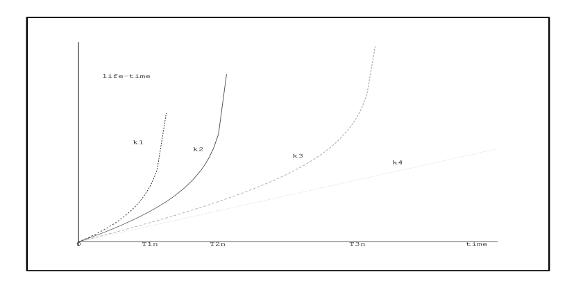
Figure 1: “Lives” of $k$ modes, for growing $k$

We can estimate the domain evolution by introducing the quantity $\Lambda_{k,n}(t)$[19, 20]:

$$e^{-2\Lambda_{k,n}(t)}\ =\ \frac{e^{-t\frac{L}{2n+1}}\,{\rm sinh}\frac{L}{2n+1}({\rm T}_{k,n}-t)}{{\rm sinh}\frac{L}{2n+1}{\rm T}_{k,n}},\qquad\,\Lambda_{k,n}(t)\ \geq 0,\,{\rm for\;any\;~{}t}~{},$$ (10)

i.e. $\Lambda_{k,n}(0)=0$ for any $k$, and $\Lambda_{k,n}(t)\rightarrow\infty$ for $t\rightarrow\ T_{k,n}$ for any given $n$. Then $\Omega_{k,n}$ may be expressed in the form:

$${\Omega_{k,n}(\Lambda_{k,n}(t))}\,=\,\Omega_{k,n}(0)e^{-\Lambda_{k,n}(t)}~{}.$$ (11)

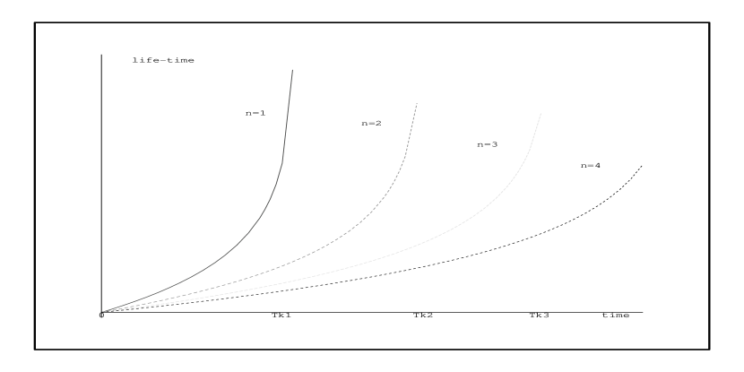
Figure 2: “Lives” of $k$ modes, for growing $n$ and fixed $k$

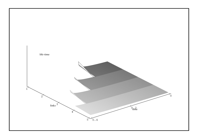
Figure 3: “Lives” of $k$ modes, for growing $n$ and ‘small‘ $k$

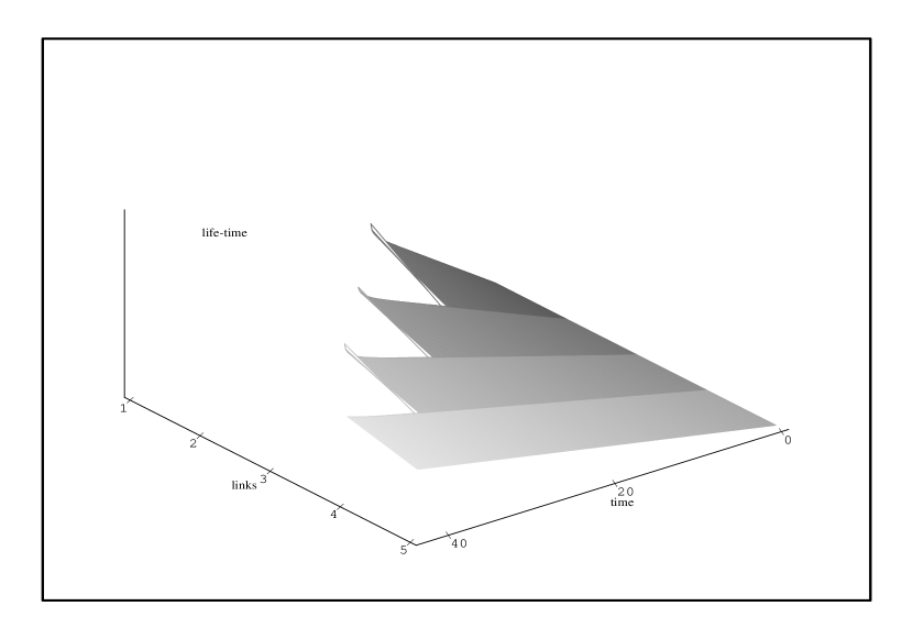
Figure 4: “Lives” of $k$ modes, for growing $n$ and ‘big‘ $k$

Since ${\Omega_{k,n}(\Lambda_{k}({\rm T}_{k,n}))}\,=\,0$, we see that $\Lambda_{k,n}(t)$ acts as a life-time, say $\tau_{k,n}$, with $\Lambda_{k,n}(t)\propto\tau_{k,n}$, for the mode $k$. Modes with larger $k$ have a ”longer” life with reference to time $t$. In other words, each $k$ mode ”lives” with a proper time $\tau_{k,n}$, so that the mode is born when $\tau_{k,n}$ is zero and it dies for $\tau_{k,n}$ $\rightarrow$ $\infty$.

The ”lives” of the $k$ modes, for growing $k$, are sketched in the figures 1-4. In Fig. 1 the lives are drawn for growing $k$ and fixed $n$ ($n=1$). Fig. 2 shows the ”lives” of a mode of given $k$ for different values of $n$. The $\Lambda_{k,n}$s are drawn versus $t$, reaching the blowing up values in correspondence of the abscissa points $T_{k,n}$. In Fig. 1 the values of $k$ have been chosen so that $k_{1}$ is one tenth of $k_{3}$ and $k_{2}$ is one tenth of $k_{4}$. Only the modes satisfying the reality condition are present at certain time $t$, being the other ones decayed. This introduces from one side an hierarchical organization of memories depending on their life-time. Memories with a specific spectrum of $k$ mode components may coexist, some of them ”dying” before, some other ones persisting longer in dependence on the number in the spectrum of the smaller or larger $k$ components, respectively (see Fig. 2). On the other hand, as observed above, since smaller or larger $k$ modes correspond to larger or smaller waves lengths, respectively, we also see that the (coherent) memory domain sizes correspondingly are larger or smaller.

In conclusion, more persistent memories (with a spectrum more populated by the higher $k$ components) are also more ”localized” than shorter term memories (with a spectrum more populated by the smaller $k$ components), which instead extend over larger domains. We have thus reached a ”graded” non-locality for memories depending on $n$ and on the spectrum of their $k$ modes components, which is also related to their life-time or persistence.

Figures 3 and 4 describe the cooperative rôle of $n$ and $k$ in supporting a long-lived memory: Fig. 3 shows the behavior of small-$k$ (with respect to $k_{0}$)modes for growing $n$ and Fig. 4 shows the behavior of large-$k$ (with respect to $k_{0}$) modes for growing $n$. It is evident that the time of memory persistence (expressed in adimensional units) increases of several orders of magnitude as the value of $k$ grows.

Since $k$ denotes the momentum of the dwq $A$ and of the $\tilde{A}$ excitations, it is expected that, for given $n$, ”more impressive” is the external stimulus (i.e. stronger is the coupling with the external world) greater is the number of high $k$ momentum excitations produced in the brain and more ”focused” is the ”locus” of the memory.

5 Final remarks and conclusions

In the quantum model of brain memory recording is obtained by coherent condensation of the dipole wave quanta in the system ground state or vacuum. In the non-dissipative case the memory states are thus stable states (infinitely long-lived states): there is no possibility to forget. On the contrary, in the dissipative case the memory states have finite (although long) life-times[8]. Above we have seen that a rich structure in the life-time behavior of single modes of momentum $k$ is implied by the frequency time-dependence of the dwq. Such a fine structure determines to some extend the memory storing ability and it appears to depend also on the brain internal parameters. There is therefore a specificity of the system which enters in determining its functional features, as of course it is natural to be. Moreover, this same fine structure also depends on the degree of openness of the brain, i.e. on the number of links which it is able to establish with the external world. On the other hand, the number of such links also turns out to be relevant to the memory recording ability.

Although at this stage our model does not give us quantitative predictions, nevertheless the qualitative behaviors and results above presented appear to fit well with the physiological observations[11] of the formation of connections among neurons as a consequence of the establishment of the links between the brain and the external world. More the brain relates to external environment, more neuronal connections will form. Connections appear thus more important in the brain functional development than the single neuron activity. Here we are referring to functional or effective connectivity, as opposed to the structural or anatomical one[11]. The last one can be described as quasi-stationary. The former one is highly dynamic with modulation time-scales in the range of hundreds of milliseconds[11]. Once these functional connections are formed, they are not necessarily fixed. On the contrary, they may quickly change in a short time and new configurations of connections may be formed extending over a domain including a larger or a smaller number of neurons. Such a picture finds a possible description in our model, where the coherent domain formation, size and life-time depend on the number of links that the brain sets with its environment and on internal parameters. As shown elsewhere (see ref. [8] and [14]) the em field propagates in ordered domains in a self-focusing fashion, thus producing an highly dynamic net of filaments and tubules which may model the highly dynamic neuronal connection assembly and disassembly. The prerequisite for the connection formation is the above described dynamic generation of ordered domains of dwq.

There is a further remarkable aspect in the occurrence of finite size domains. The finiteness of the domain size spoils the unitary inequivalence among the vacua of the domain. Then, in the case of open systems, transitions among (would be) unitary inequivalent vacua may occur (phase transitions) for large but finite volume, due to coupling with external environment.It has been shown that small perturbation may drive the system through its vacua[21]. In this way occasional (random) perturbations may play an important rôle in the complex behavior of the brain activity. However, transitions among different vacua may be not a completely negative feature of the model: once transitions are allowed, the possibility of associations of memories (”following a path of memories”) becomes possible. Of course, these ”transitions” should only be allowed up to a certain degree in order to avoid memory ”confusion” and difficulties in the process of storing ”distinct” memories. The opposite situation of strict inequivalence among different vacua (in the case of very large or infinite size domain) would correspond to the absence of any ”transition” among memory states and thus to ”fixation” or ”trapping” in some specific memory state.

In connection with the recall mechanism, we note (see ref. [8]) that the dwq acquires an effective non-zero mass due to the domain finite size. Such an effective mass will then acts as a threshold in the excitation energy of dwq so that, in order to trigger the recall process an energy supply equal or greater than such a threshold is required. When the energy supply is lower than the required threshold a ”difficulty in recalling” may be experienced. At the same time, however, the threshold may positively act as a ”protection” against unwanted perturbations (including thermalization) and cooperate to the stability of the memory state. In the case of zero threshold (infinite size domain) any replication signal could excite the recalling and the brain would fall in a state of ”continuous flow of memories”.

We further observe that the differences in the life-time of the $k$ components may produce the corruption of the spectral structure of the memory information (of the memory code) with consequent more or less severe memory ”deformations”. On the other hand, due to the dissipation, at some time $t=\tau$, conveniently larger than the memory life-time, the memory state $|0>_{\cal N}$ is reduced to the ”empty” vacuum $|0>_{0}$ where ${\cal N}_{\kappa}=0$ for all $\kappa$: the information has been forgotten. At the time $t=\tau$ the state $|0>_{0}$ is available for recording a new information. In order to not completely forget certain information, one needs to ”restore” the ${\cal N}$ code, namely to ”refresh” the memory by brushing up the subject (external stimuli maintained memory).

Finally, we note that one is actually obliged to consider the dissipative, irreversible time-evolution: in fact after information has been recorded, the brain state is completely determined and the brain cannot be brought to the state in which it was before the information printing occurred. Thus, the same fact of getting information introduces the arrow of time into brain dynamics. In other words, it introduces a partition in the time evolution, namely the distinction between the past and the future, a distinction which did not exist before the information recording. It can be shown that dissipation and the frequency time-dependence imply that the evolution of the memory state is controlled by the entropy variations[8]: this feature reflects indeed the irreversibility of time evolution (breakdown of time-reversal symmetry). The stationary condition for the free energy functional leads then to recognize the memory state $|0(t)>_{\cal N}$ to be a finite temperature state[13], which opens the way to the possibility of thermodynamic considerations in the brain activity. In this connection we observe that the “psychological arrow of time” which emerges in the brain dynamics turns out point in the same direction of the “thermodynamical arrow of time”, which points in the increasing entropy direction. It is interesting to note that both these arrows, the psychological one and the thermodynamical one, also point in the same direction of the ”cosmological arrow of time” defined by the expanding Universe direction[20, 22]. On the subject of the concordance of the three different arrows of time there is an interesting debate still going on(see e.g. [22]). It is remarkable that the dissipative quantum model of brain let us reach a conclusion on the psychological arrow of time which we commonly experience.

This work has been partially supported by INFM and by MURST.

6 Appendix

We briefly summarize the main steps in the quantization procedure of the eqs. (1). For more details see refs. [15, 19, 20] where, although in a different context, a complete treatment is given. In the following we will omit the suffices for simplicity, unless they are needed in order to avoid misunderstanding. It turns out to be convenient to introduce the canonical transformations

$$u(t)\ =\ \frac{U(t)+V(t)}{\sqrt{2}},\qquad v(t)\ =\ \frac{U(t)-V(t)}{\sqrt{2}}.$$ (12)

The Hamiltonian for our coupled oscillator equations is:

$${\cal H}={1\over 2}{p_{U}}^{2}+{1\over 2}{\Omega}^{2}(t)U^{2}-{1\over 2}{p_{V}}^{2}-{1\over 2}{\Omega}^{2}(t)V^{2}-{\Gamma}({p_{U}}V+{p_{V}}U).$$ (13)

with $\Gamma\equiv{L\over 2}$. We assume $\Omega(t)$ to be real (for any $k$ and any $t$) in order to avoid over-damped regime. As we have discussed in the text, this condition acts as a cut-off on $k$. The conjugate momenta are

$$p_{U}=\dot{U}+{L\over 2}V~{}~{},\qquad p_{V}=-\dot{V}-{L\over 2}U~{}~{}.$$ (14)

We introduce the annihilation operators

$$A=\frac{1}{\sqrt{2}}\left(\frac{p_{U}}{\sqrt{\hbar\omega_{0}}}-iU\sqrt{\frac{\omega_{0}}{\hbar}}\right),\qquad{\tilde{A}}=\frac{1}{\sqrt{2}}\left(\frac{p_{V}}{\sqrt{\hbar\omega_{0}}}-iV\sqrt{\frac{\omega_{0}}{\hbar}}\right),$$ (15)

and the corresponding creation operators with usual commutation relations. Here $\omega_{0}$ is an arbitrary constant frequency. Then it can be shown that the vacuum state $|0>$ is unstable:

$$<0(t)|0>\,\propto\exp{\left(-t\Gamma\right)}\rightarrow 0\;~{}for~{}large~{}t,$$ (16)

i.e. time evolution brings ”out” of the initial-time Hilbert space for large $t$. This compels us to work in the framework of QFT (not just of Quantum Mechanics!)[19]. In order to set up the formalism in QFT we have to consider the infinite volume limit; however, as customary, we will work at finite volume and at the end of the computations we take the limit $V\rightarrow\infty$. The QFT Hamiltonian is

$${\cal H}={\cal H}_{0}+{\cal H}_{I_{1}}+{\cal H}_{I_{2}}$$ (17)

$${\cal H}_{0}=\sum_{k}\frac{1}{2}\hbar\Omega_{0,{k}}(t)(A^{\dagger}_{k}A_{k}-{\tilde{A}}^{\dagger}_{k}{\tilde{A}}_{k})~{},$$ (18)

$${\cal H}_{I_{1}}=-\sum_{k}{1\over 4}\hbar\Omega_{1,{k}}(t)\left[\left(A_{k}^{2}+{A^{\dagger 2}_{k}}\right)-\left({{\tilde{A}}_{k}}^{2}+{{\tilde{A}}^{\dagger 2}_{k}}\right)\right]~{},$$ (19)

$${\cal H}_{I_{2}}=i\sum_{k}{\Gamma}_{k}{\hbar}\left(A^{\dagger}_{k}{\tilde{A}}^{\dagger}_{k}-A_{k}{\tilde{A}}_{k}\right)~{},$$ (20)

with $\Omega_{0,1,k}=\omega_{0}\left(\frac{{{\Omega}_{k}}^{2}(t)}{\omega^{2}_{0}}\pm 1\right)~{}~{}$ and

$$[A_{k},A^{\dagger}_{{k}^{\prime}}]={\delta}_{{k},{k}^{\prime}}=[{\tilde{A}}_{k},{\tilde{A}}^{\dagger}_{{k}^{\prime}}],\qquad{[}A_{k},{\tilde{A}}_{{k}^{\prime}}{]}=0\,=\,[A^{\dagger}_{k},{\tilde{A}}^{\dagger}_{{k}^{\prime}}].$$ (21)

We remark that

$$[{\cal H}_{0},{\cal H}_{I_{2}}]=0=[{\cal H}_{I_{1}},{\cal H}_{I_{2}}]~{},$$ (22)

which guarantees that the minus sign appearing in ${\cal H}_{0}$ is not harmful, i.e., once one starts with a positive definite Hamiltonian it remains lower bounded under time evolution.

By using the transformation ${\cal H}\rightarrow{{\cal H}^{\prime}}\equiv S(\theta)^{-1}{\cal H}S(\theta)$ with $S(\theta)\equiv\prod_{k}e^{-i\theta_{k}(t)K_{2,k}}$ and

$$\tanh{\theta_{k}(t)}=-{\Omega_{1,k}(t)\over\Omega_{0,k}(t)}$$ (23)

at any $t$ for any given $k$ we can ”rotate away” ${\cal H}_{I_{1}}$:

$${{\cal H}^{\prime}}\equiv S(\theta)^{-1}{\cal H}S(\theta)={\cal H}^{\prime}_{0}+{\cal H}_{I_{2}}~{}~{}.$$ (24)

Note that

$${{\cal H}^{\prime}}_{0}=\sum_{k}\hbar\Omega_{k}(t)(A_{k}^{\dagger}A_{k}-{\tilde{A}}_{k}^{\dagger}{\tilde{A}}_{k})~{}~{},$$ (25)

and $[{{\cal H}^{\prime}}_{0},{\cal H}_{I_{2}}]=0$. When the initial state, say at arbitrary initial time $t_{0}$, ($t_{0}=0$, ${\theta}_{k}({0})\equiv{\theta}_{k}$ for sake of simplicity) is the vacuum $|0>$ for ${{\cal H}^{\prime}}_{0}$, with $A_{k}|0>=0={\tilde{A}}_{k}|0>$, the state $|0(\theta)>=S(\theta)|0>~{}$ is the zero energy eigenstate (the vacuum) of ${\cal H}_{0}+{\cal H}_{I_{1}}$ at $t_{0}$:

$$({\cal H}_{0}+{\cal H}_{I_{1}})|_{t_{0}}|0(\theta)>=S(\theta){\cal H}^{\prime}_{0}|0>=0.~{}~{}$$ (26)

We observe that the operators $A_{k}$ and ${\tilde{A}}_{k}$ transform under $\exp{\left(-i{\theta}_{k}K_{2,k}\right)}$ as

$$A_{k}\mapsto A_{k}(\theta)={\it e}^{-i{\theta}_{k}K_{2,k}}A_{k}{\it e}^{i{\theta}_{k}K_{2,k}}=A_{k}\cosh{(\frac{1}{2}{\theta}_{k})}+{A_{k}}^{\dagger}\sinh{(\frac{1}{2}{\theta}_{k})}~{},$$ (27)

$${\tilde{A}}_{k}\mapsto{\tilde{A}}_{k}(\theta)={\it e}^{-i{\theta}_{k}K_{2,k}}{\tilde{A}}_{k}{\it e}^{i{\theta}_{k}K_{2,k}}={\tilde{A}}_{k}\cosh{(\frac{1}{2}{\theta}_{k})}+{{\tilde{A}}_{k}}^{\dagger}\sinh{(\frac{1}{2}{\theta}_{k})}~{}.$$ (28)

One has $A_{k}(\theta)|0(\theta)>=0={\tilde{A}}_{k}(\theta)|0(\theta)>$ .

The $t$-evolution of the vacuum $|0(\theta)>$ is obtained as (at finite volume $V$):

$$|0(\theta,t)>=\prod_{k}{1\over{\cosh{(\Gamma_{k}t)}}}\exp{\left(\tanh{(\Gamma_{k}t)}J_{{k},+}(\theta)\right)}|0(\theta)>\quad,$$ (29)

with $J_{k,+}(\theta)=A^{\dagger}_{k}(\theta){\tilde{A}}^{\dagger}_{k}(\theta)$. We have $A_{k}(\theta,t)|0(\theta,t)>=0={\tilde{A}}_{k}(\theta,t)|0(\theta,t)>$ with

$$A_{k}(\theta)\mapsto A_{k}(\theta,t)={\it e}^{-i{t\over{\hbar}}{\cal H}_{I_{2}}}A_{k}(\theta){\it e}^{i{t\over{\hbar}}{\cal H}_{I_{2}}}=A_{k}(\theta)\cosh{({\Gamma}_{k}t)}-{\tilde{A}}_{k}(\theta)^{\dagger}\sinh{({\Gamma}_{k}t)}\quad,$$ (30)

$${\tilde{A}}_{k}(\theta)\mapsto{\tilde{A}}_{k}(\theta,t)={\it e}^{-i{t\over{\hbar}}{\cal H}_{I_{2}}}{\tilde{A}}_{k}(\theta){\it e}^{i{t\over{\hbar}}{\cal H}_{I_{2}}}=-A_{k}(\theta)^{\dagger}\sinh{({\Gamma}_{k}t)}+{\tilde{A}}_{k}(\theta)\cosh{({\Gamma}_{k}t)}\quad.$$ (31)

Notice that these are the time-dependent, canonical Bogolubov transformations.

The state $|0({\theta},t)>$ is a normalized state,  $<0(\theta,t)|0(\theta,t)>=1\quad\forall t$,  and is a $su(1,1)$ generalized coherent state. It can be shown that in the infinite volume limit

$$<0(\theta,t)|0(\theta)>{\smash{\mathop{\longrightarrow}\limits_{V\rightarrow\infty}}}0\quad\forall\,t\quad,$$ (32)

$$<0(\theta,t)|0(\theta^{\prime},t^{\prime})>{\smash{\mathop{\longrightarrow}\limits_{V\rightarrow\infty}}}0\quad with~{}~{}\theta^{\prime}\equiv\theta(t_{0}^{\prime}),~{}~{}\forall\,t\,,t^{\prime}\,,t_{0}^{\prime}\quad,\quad t\neq t^{\prime}~{}~{}.$$ (33)

Eqs. (32) and (33) show that in the infinite volume limit the vacua at $t$ and at $t^{\prime}$, for any $t$ and $t^{\prime}$, are orthogonal states and thus the corresponding Hilbert spaces are unitarily inequivalent spaces.

The number of modes of type $A_{k}(\theta)$ in the state $|0(\theta,t)>$ is given, at each instant $t$ by

$${N}_{A_{k}}(t)\equiv<0(\theta,t)|A_{k}^{\dagger}(\theta)A_{k}(\theta)|0(\theta,t)>=\sinh^{2}\bigl{(}\Gamma_{k}t\bigr{)}\quad,$$ (34)

and similarly for the modes of type ${\tilde{A}}_{k}(\theta)$.

We also observe that the number $\left(N_{A_{k}}-N_{{\tilde{A}}_{k}}\right)\,$ is a constant of motion for any $k$ and any $\theta$. Moreover, one can show that the creation of a mode $A_{k}(\theta)$ is equivalent to the destruction of a mode ${\tilde{A}}_{k}(\theta)$ and vice-versa. This means that the ${\tilde{A}}_{k}(\theta)$ modes can be interpreted as the holes for the modes $A_{k}(\theta)$: the ${\tilde{A}}$ system can be considered as the sink where the energy dissipated by the $A$ system flows.

Finally thermal properties of the vacuum $|0(\theta,t)>$ can be analyzed[15, 19, 20] and the $\tilde{A}$ modes appear to represent the thermal bath (the environment) modes.

References

- [1] K.H.Pribram, Brain and perception, Lawrence Erlbaum, New Jersey, 1991
- [2] K.H.Pribram, Languages of the brain, Englewood Cliffs, New Jersey, 1971
- [3] L.M.Ricciardi and H.Umezawa, Kibernetik 4, 44 (1967)
- [4] C.I.J.Stuart, Y.Takahashi and H.Umezawa, J. Theor. Biol. 71, 605 (1978)
- [5] C.I.J.Stuart, Y.Takahashi and H. Umezawa, Found. Phys. 9, 301 (1979)
- [6] S. Sivakami and V. Srinivasan, J. Theor. Biol. 102, 287 (1983)
- [7] M.Jibu , K.H.Pribram and K.Yasue, Int. J. Mod. Phys. B10, 1735 (1996)
- [8] G. Vitiello, Int. J. Mod. Phys. 9, 973 (1995)
- [9] E.Pessa and G.Vitiello, Biolectrochemistry and bioenergetics 48, 339 (1999)
- [10] M. Rasetti, What is quantum computation? A review and an update, Politecnico di Torino, Preprint, J. Preskill, Fault-tolerant quantum computation, Proceedings of: ”Introduction to Quantum Computation,” edited by H.-K. Lo, S. Popescu, and T. P. Spiller,quant-ph/9712048
- [11] S.A.Greenfield, Communication and Cognition 30, 285 (1997)
- [12] C. Itzykson and J. Zuber, Quantum field theory, McGraw-Hill Book Co., N.Y., 1980
- [13] H.Umezawa, Advanced field theory: micro, macro and thermal concepts, American Institute of Physics, N.Y. 1993
- [14] E.Del Giudice, S.Doglia, M.Milani and G.Vitiello, Nucl. Phys. B275 [FS 17], 185 (1986); in Biological coherence and response to external stimuli, ed. H.Fröhlich (Springer-Verlag, Berlin 1988), p.49
- [15] E. Celeghini, M. Rasetti and G. Vitiello, Ann.Phys. (N.Y.) 215, 156 (1992)
- [16] M.Abramowitz and I.A.Stegun, Handbook of Mathematical Functions (Dover Pub. N.Y. 1970)
- [17] V. I. Smirnov, Kurs vyssej matematiki (Mir)
- [18] J.D.Jackson, Classical Electrodynamics (Wiley and Sons. 1975)
- [19] E. Alfinito and G. Vitiello Phys. Lett. A 252, , (5) (1999)
- [20] E.Alfinito, R.Manḱa and G.Vitiello, Class.Quant.Grav 17, 93 (2000)
- [21] E.Celeghini, E.Graziano and G.Vitiello, Phys. Lett. A145, 1 (1990)
-
[22]
S.W.Hawking Phys. Rev. D32, 2389 (1985)
S.W.Hawking and R.Penrose, The Nature of Space and Time (Princeton University Press 1996)