Discrete Phase Measurements and the Bell inequality

Abstract

We present a formulation of the Bell inequalities using simple correlated photon number states and phase measurements. Such tests generally require binning of the information, and this effect is closely examined. Our proposal opens up the opportunity for a new novel test of quantum mechanics versus local realism. Some insight in entanglement in such systems may be achieved.

I Introduction

The Bell inequalities[2, 3, 4] and their tests of quantum mechanics have generally been seen only as a fundamental test of quantum mechanics[5] until recently. Now however their relevance has become much more important with the proposal for quantum computing and quantum encryption. Fundamental to these schemes is quantum entanglement which is at the core of quantum mechanics. The Bell inequalities provide a mechanism now by which strongly[6] entangled two mode systems can be distinguished from all classical systems. Current tests of the Bell inequalities have suffered from a number of loopholes [3, 7, 8, 9], including the fair sampling assumption and low detection efficiencies. To date, no definitive experiment test has been achieved although specific experiments have been performed which close one or more of the loopholes. This has lead to proposals from a number of authors including ourselves [10, 11, 12, 13, 14] to consider high efficiency detection. Work by Smithery et. al.[15] has indicated how high efficiency photon detectors can be used to detect large photon numbers but with an uncertainty in the actual photon number. Reid et. al.[10] indicated how high efficiency photon detectors, with large particle numbers, can test macroscopic quantum mechanics.

In a recent paper by Gilchrist et. al.[11] they showed how the predictions of quantum mechanics are in disagreement with those of local hidden variable theories for a situation involving continuous quadrature phase amplitude ( position and momentum ) measurements. More explicitly they showed that the quantum predictions for the probability of obtaining results $x$ and $p$ for position and momentum (or various linear combinations) cannot be predicted by any local hidden variable theory. The test could be achieved by binning the continuous position and momentum information into two and using the binary results in the strong Clauser Horne Bell inequality test[4]. There predicted violation was small (less than 2%). Munro [12] considered various different strong Bell inequalities and indicated how larger violations may be achieved.

Also published at a similar time by us [13] we proposed how the novel use of phase measurements on a simple correlated photon number triplet could be used to test the GHZ correlations via the Mermin $F$ inequality[16]. More explicitly we showed how simple correlated photon number triplets which ideally could be produced in nondegenerate parametric oscillation, where we have signal, idler and pump modes, in conjunction with discrete binary phase measurements could be used to provide a definitive test of quantum mechanics versus all local realism. In fact a maximal violation of the mermin $F$ inequality was indicated. However as we mentioned in this paper discrete phase measurements in optical systems have yet to be experimentally realized in the ultra high detector efficiency limit. As an approximation to this binary phase measurement a homodyne quadrature phase amplitude measurements was considered and also found to violate the inequality. The potential violation is significantly reduced however because information in the quadrature phase amplitude measurements must be discarded to achieve the binary result.

In this paper we will be restricting our attention to systems involving correlated photon number states. To obtain the maximum entanglement information we are proposing the use of canonical phase measurements. Initially we consider a discrete binary phase measurement but then generalise to phase measurements involving larger (greater than two) numbers of phase results. To achieve a Bell inequality test in such cases requires binning of the results from the phase measurements. A critical part of this paper is to determine the effect of this binning process. Until recently only two limits have been considered, binary discrete phase measurements and continuous quadrature phase amplitude measurements. We analyse a number of cases between these extreme limits. While our phase measurements may not be easily experimentally achievable valuable insight into the binning of data for the Bell inequalities is obtained. While we will not explicitly consider correlated spin systems, the results indicated by the binning of phases could be applied to these spin systems. For instance with binning a correlated $3/2$ system could be used to test the Bell inequality. Historically only correlated $1/2$ systems have been used. This opening the possibility for new novel tests of quantum mechanics with higher spin particles.

II Entanglement

It is important to begin by explaining the reason for considering phase measurements especially when we are restricting our attention to correlated photon number state systems. As has long been known quantum entangled states shows correlations that cannot be explained in terms of the correlations between local classical properties of the subsystems. In this paper we are describing a pure entangled state of two modes in which the correlations are in photon number, that is the nature of correlation can be succinctly stated by saying that there are equal number of photons in each mode. Now as there are many different ways to realize this, the total state is the sum over amplitudes for all possible ways in which this correlation can be realized. This kind of sum over amplitudes for correlations is characteristic of an entangled state.

How do we best see the quantum nature of the correlation? Obviously it is not enough to measure photon number as this would not distinguish a mixed state, with equal photon numbers in each mode, from the equivalent entangled pure state. In some sense we need to measure an observable which carries as little information as possible about photon number in order to see the interference between all the possible ways in which the correlation in photon number can be realized. We conjecture that the best choice is the observable canonically conjugate to photon number; the phase. Before we consider the quantum mechanical phase (Section IV) we will in the next section specify more precisely the nature of the entangled states we are considering and realisable systems that generate them.

III Entangled Photon Pair States

Tests of quantum mechanics generally require an entanglement between particles. A test of the Bell inequality requires an entanglement between two subsystems. As mentioned previously we are examining a two mode state where there are an equal number of photons in each mode. This correlated photon number pair state is given by

$$|\Psi\rangle=\sum_{n=0}^{\infty}c_{n}|n\rangle|n\rangle$$ (1)

where at present we leave $c_{n}$ arbitrary but specify that due to normalisation

$$\sum_{n=0}^{\infty}\left|c_{n}\right|^{2}=1.$$ (2)

For convenience in the calculations that follow, we will place the condition on $c_{n}$ that it must be real. Eqn (1) actually describes a number of idealised but real systems. The most well known and extensively examined case is the nondegenerate parametric amplifier specified by an ideal Hamiltonian of the form[17]

$$H=-\hbar\chi\epsilon\left(ab+a^{\dagger}b^{\dagger}\right).$$ (3)

where $\epsilon$ is field amplitude of a nondepleting classical pump and $\chi$ is proportional to the susceptibility of the medium. $a,b$ are the boson operators for the two spatially separated orthogonal signal and idler modes systems. After a time $\tau$, the state of the system is given by (1) with $c_{n}$ specified by

$$c_{n}={{\tanh^{n}\left[\chi\epsilon\tau\right]}\over{\cosh\left[\chi\epsilon\tau\right]}}$$ (4)

For small $\chi\epsilon\tau$ in Eqn (4) a state of the form

$$|\Psi\rangle=c_{0}|0\rangle|0\rangle+c_{1}|1\rangle|1\rangle$$ (5)

can be generated as a reasonably good approximation.

Another source of highly correlated photon number states exists in the steady state by nondegenerate parametric oscillation [18] as modeled by the following Hamiltonian,

$$H=-i\hbar\epsilon\left(ab-a^{\dagger}b^{\dagger}\right)+ab\Gamma^{\dagger}+a^{\dagger}b^{\dagger}\Gamma.$$ (6)

Here we have neglected the effect of linear single photon loss. We assume that the coupled signal-idler loss dominates over linear single-photon loss. In Eqn. (6) $\epsilon$ represents a coherent driving source which generates signal-idler pairs, while $\Gamma$ represents the reservoir systems which gives rise to the coupled signal-idler loss. $a,b$ again are the boson operators for the orthogonal signal and idler modes. In the limit of very large parametric nonlinearity and high Q cavities, a state of the form[18]

$$|{\mbox{circle}}\rangle={\mathcal{N}}\int_{0}^{2\pi}|re^{i\varsigma}\rangle_{a}|re^{-i\varsigma}\rangle_{b}d\varsigma$$ (7)

can be generated. Here ${\mathcal{N}}$ is the normalisation coefficient while $|{\ldots}\rangle_{a}$ and $|{\ldots}\rangle_{b}$ are coherent states of amplitude $r$ in the spatially separated modes $\hat{a}$ and $\hat{b}$. This state can be written in the form of eqn (1) with the $c_{n}$’s now specified by

$$c_{n}={{r^{2n}}\over{n!I_{0}\left(2r^{2}\right)}}$$ (8)

where $I_{0}$ is the zeroth order modified Bessel function.

Given that we now have exactly specified the nature of the our correlation we return to consider the observable canonically conjugate to photon number; the phase.

IV Phase states

Above we have proposed that that phase states may be the best way to observe entanglement in photon number. There have been a number of phase states proposed over recent years[19, 20, 21, 22, 23]. A canonical phase state[19, 20, 21] $|\theta\rangle$ can be generally be defined as

$$|\theta\rangle={1\over\sqrt{2\pi}}\sum_{n=0}^{\infty}\exp\left[in\theta\right]|n\rangle$$ (9)

where $|n\rangle$ represent the fock states and $\theta$ specifies the phase. These phase states are unnormalized as $\langle\theta|\theta\rangle>1$. In fact they are unnormalisable. A normalizable phase state was proposed by Pegg and Barnett[22, 23] who considered the phase state definition

$$|\theta\rangle=\lim_{s\rightarrow\infty}{1\over\sqrt{s+1}}\sum_{n=0}^{s}\exp\left[in\theta\right]|n\rangle.$$ (10)

Here $|n\rangle$ are the $s+1$ number states that span the $(s+1)$ dimensional state space. The limit in Eqn (10) is absolutely necessary in order to normalize the states. The parameter $\theta$ can take on any real value, although distinct states will occur in a $2\pi$ range.

Pegg and Barnett[22, 23] showed that a set of $s+1$ orthonormal phase states, with values of $\theta$ differing by $2\pi/(s+1)$, can be generated from

$$|\theta_{\mu}\rangle=\exp\left[i\hat{N}\mu 2\pi/(s+1)\right]|\theta_{0}\rangle,\;\;\mu=0,\ldots,s$$ (11)

where $|\theta_{0}\rangle$ is the reference (or zero) phase state. Here $\hat{N}$ is the number operator and $\mu$ the particular discrete phase we are interested in. $\mu$ generally varies in integer steps from $0$ to $s$. Our values for $\theta_{\mu}$ are given by

$$\theta_{\mu}=\theta_{0}+{{2\mu\pi}\over{(s+1)}}$$ (12)

which are spread evenly over the range $\theta_{0}\leq\theta_{\mu}\leq\theta_{0}+2\pi$, where $\theta_{0}$ is the initial (or reference) phase.

V Probability distributions

Now given the form (1) and the definition of discrete phase states in section (IV) we now proceed to calculate the joint probability of finding our correlated photon number system with phase $\theta_{\mu_{1}}$ for in the first subsystem/mode and $\theta_{\mu_{2}}$ for the second subsystem/mode. We specify that there is an initial phase angle $\theta_{0,i}$ for each of the subsystems $i$ (i=1,2). The joint probability $P_{\mu_{1},\mu_{2}}\left(\theta_{0,1},\theta_{0,2}\right)$ is given by

$$P_{\mu_{1},\mu_{2}}\left(\theta_{0,1},\theta_{0,2}\right) = \sum_{n=0}^{s}{{\left|c_{n}\right|^{2}}\over{\left(s+1\right)^{2}}}+\sum_{n>n^{\prime}=0}^{s}{{2c_{n}c_{n^{\prime}}}\over{\left(s+1\right)^{2}}}$$ (13)

$$\times \cos\left[\Delta n\left({{2\pi\left[\mu_{1}+\mu_{2}\right]}\over{s+1}}+\psi_{0}\right)\right]$$ (14)

Here $\psi_{0}$ is the sum of the two initial phase angle ($\psi_{0}=\theta_{0,1}+\theta_{0,2}$) and $\Delta n=n-n^{\prime}$. Here each $\mu_{i}$ can vary from $0$ to $s$ in integer steps.

It is useful to calculate the marginal probability $P_{\mu_{i}}\left(\theta_{0,i}\right)$ (where $i$ equals either 1 or 2) of finding the correlated photon number system with phase $\theta_{\mu_{i}}$ for the ${\rm i^{th}}$ subsystem (i=1,2), while having no information about the remaining subsystem (that is the remaining subsystem may be in any phase state). Here the marginal probability $P_{\mu_{i}}\left(\theta_{0,i}\right)$ is given by

$$P_{\mu_{i}}\left(\theta_{0,i}\right)={1\over{s+1}}\sum_{n=0}^{s}\left|c_{n}\right|^{2}$$ (15)

It is interesting to note that $P_{\mu_{i}}\left(\theta_{0,i}\right)$ is actually independent of all angular dependence, both from $\mu_{i}$ and $\theta_{0,i}$, the initial or reference choice of phase for that subsystem. In fact the marginal probability is uniformly distributed over all the possible results. In the limit that $s$ becomes very large $P_{\mu_{i}}\left(\theta_{0,i}\right)\rightarrow 0$.

VI Binary Choice

We generally require large $s$ to describe an arbitrary phase for a general system. In fact to specify the phase as precisely as possible we require $s\rightarrow\infty$. However in the case of the measurement schemes required for testing the various quantum paradox such as the Bell inequalities, all that is required and actually necessary is a binary result [24]. Hence it would be logical to have a discrete phase measurement with say $s=1$, that is only two phase states. Such a scheme has been analyzed by Munro and Milburn[13] for the GHZ state.

It may not always be possible to have only two phase states. If more phase states are present (for example $s=3$), a binary result is still required for these particular quantum paradoxes (and especially the Bell inequalities we are interested in, although some of the inequalities such as the Information theoretic Bell inequality[25] or the Mermin higher spin inequality[16] allow for other than a binary result). This could be achieved by dividing or binning the phase states into two discrete distinct sets. We could for instance label $P_{\uparrow,\uparrow}\left(\theta_{0,1},\theta_{0,2}\right)$ as the probability of finding both particles in a $\uparrow$ state (where the $\uparrow$ state is one of the two possible binary results, the other being $\downarrow$). $P_{\downarrow,\downarrow}\left(\theta_{0,1},\theta_{0,2}\right)$ would correspond to the probability of finding both modes in the $\downarrow$ state. How exactly this binary choice is achieved will be discussed on a per case basis in the next few sections of this paper. We could for instance specify that an $\uparrow$ result corresponds results containing the phase results $\mu=0\ldots s/2$. Such a process however discards information about the system and hence we would expect a lessening of our potential Bell inequality violation.

VII The Bell inequalities

A number of Bell inequalities exist, and the particular one to be considered in this article are the Clauser Horne[4] and the spin[2] Bell inequality. A detailed derivation of the various inequalities will not be given, the reader is referred to references [2, 4]. In Fig (1) we depict a very idealized setup for general Bell inequality experiment.

To formulate the Bell inequalities it is necessary to postulate the existence of a local hidden variable theory. We can write the probability $P_{\uparrow,\uparrow}\left(\theta_{0,1},\theta_{0,2}\right)$ for obtaining a result $\uparrow$ and $\uparrow$ respectively upon the simultaneous measurements the phase at $A$ and the phase at $B$ in terms of the hidden variables $\lambda$ as

$$P_{\uparrow,\uparrow}\left(\theta_{0,1},\theta_{0,2}\right)=\int\rho(\lambda)p_{\uparrow}^{A}(\theta_{1,0},\lambda)p_{\uparrow}^{B}(\theta_{2,0},\lambda)d\lambda$$ (16)

The $\rho(\lambda)$ is the probability distribution for the hidden variable state denoted by $\lambda$. $p_{\uparrow}^{A}(\theta_{0,2},\lambda)$ is the probability of obtaining a result $\uparrow$ upon measurement at $A$ of the phase, given the hidden variable state $\lambda$. Similarly $p_{\uparrow}^{B}(\theta_{0,2},\lambda)$ is the probability of obtaining a result $\uparrow$ upon measurement at $B$ of the phase, also given the hidden variable state $\lambda$. Our locality assumption is due to the fact that a measurement at $A$ cannot be influenced by the choice of parameter $\theta_{2,0}$ at the location $B$ (and vice versa).

A number of Bell inequalities exist and in this article we will consider only two cases. The first is the strong Clauser-Horne Bell inequality that can then be written in the form of

$$|{\bf B}_{\rm{CH}}|\leq 1$$ (17)

where

$$B_{\rm{CH}}={{P_{\uparrow\uparrow}\left(\theta_{1,0},\theta_{2,0}\right)-P_{\uparrow\uparrow}\left(\theta_{1,0},\theta_{2,0}^{\prime}\right)+P_{\uparrow\uparrow}\left(\theta_{1,0}^{\prime},\theta_{2,0}\right)+P_{\uparrow\uparrow}\left(\theta_{1,0}^{\prime},\theta_{2,0}^{\prime}\right)}\over{P_{\uparrow}\left(\theta_{1,0}^{\prime}\right)+P_{1}\left(\theta_{2,0}\right)}}$$ (18)

Here $P_{\uparrow\uparrow}$ is the probability that a “$\uparrow\uparrow$” results occurs at each analyzer $A,B$ given $\theta_{1,0}$,$\theta_{2,0}$. Similarly $P_{\uparrow}$ is the probability that a “$\uparrow$” occurs at a detector while having no information about the second. For many of the actual experimental considerations an angle factorization occurs so that $P_{\uparrow\uparrow}\left(\theta_{1,0},\theta_{2,0}\right)$ depends only on $\theta_{1,0}+\theta_{2,0}$. Also $P_{\uparrow}\left(\theta_{i,0}\right)$ is independent of both $\theta_{1,0},\theta_{2,0}$. In this case $B_{\rm{CH}}$ can be simplified to

$$B_{\rm{CH}}={{2P_{\uparrow\uparrow}\left(\psi\right)+P_{\uparrow\uparrow}\left(-\psi\right)-P_{\uparrow\uparrow}\left(3\psi\right)}\over{2P_{\uparrow}}}$$ (19)

where $\psi=\theta_{1,0}+\theta_{2,0}=-\theta_{1,0}^{\prime}-\theta_{2,0}^{\prime}=\theta_{1,0}+\theta_{2,0}^{\prime}$ and $3\psi=\theta_{1,0}^{\prime}+\theta_{2,0}$. In some cases it can be shown that $P_{\uparrow\uparrow}\left(\psi\right)=P_{\uparrow\uparrow}\left(-\psi\right)$ and hence this expression further simplifies to

$$B_{\rm{CH}}={{3P_{\uparrow\uparrow}\left(\psi\right)-P_{\uparrow\uparrow}\left(3\psi\right)}\over{2P_{\uparrow}}}$$ (20)

This is the commonly used form for ${\bf B}_{\rm{CH}}$. A violation of this strong Clauser Horne Bell inequality is possible if $|{\bf B}_{\rm{CH}}|>1$.

The second form of the Bell inequality (sometimes referred to as the spin or original Bell inequality) is given by[2]

$$|B_{\rm S}|\leq 2$$ (21)

where

$$B_{\rm S}=|E\left(\theta_{1,0},\theta_{2,0}\right) - E\left(\theta_{1,0},\theta_{2,0}^{\prime}\right)$$ (22)

$$+ E\left(\theta_{1,0}^{\prime},\theta_{2,0}\right)+E\left(\theta_{1,0}^{\prime},\theta_{2,0}^{\prime}\right)|\leq 2$$ (23)

Here the correlation function $E\left(\theta_{1,0},\theta_{2,0}\right)$ is given by

$$E\left(\theta_{1,0},\theta_{2,0}\right) = P_{\uparrow\uparrow}\left(\theta_{1,0},\theta_{2,0}\right)+P_{\downarrow\downarrow}\left(\theta_{1,0},\theta_{2,0}\right)$$ (24)

$$- P_{\uparrow\downarrow}\left(\theta_{1,0},\theta_{2,0}\right)-P_{\downarrow\uparrow}\left(\theta_{1,0},\theta_{2,0}\right)$$ (25)

As has been discussed above $P_{\uparrow\uparrow}$ is probability that a “$\uparrow$” results occurs at each analyzer $A,B$ given $\theta_{1,0},\theta_{2,0}$. $P_{\downarrow\downarrow}$ is probability that a “$\downarrow$” results occurs at each analyzer $A,B$, while $P_{\uparrow\downarrow}$ ($P_{\downarrow\uparrow}$) is probability that a “$\uparrow$” (“$\downarrow$”) results occurs at the analyzer $A$ and a “$\downarrow$” (“$\uparrow$”) at $B$. With the angle factorization given above, the inequality (21) can be rewritten as

$$B_{\rm S}=2E\left(\psi\right)+E\left(-\psi\right)-E\left(3\psi\right)$$ (26)

When $E\left(\psi\right)=E\left(-\psi\right)$ this expression further simplifies to

$$B_{\rm S}=3E\left(\psi\right)-E\left(3\psi\right)$$ (27)

A violation of this inequality is possible if $|{\bf B}_{\rm{S}}|>2$.

These are the two Bell inequalities that will be tested with our ideal correlated photon pairs and phase states.

VIII Binary Phase Measurements

As has been mentioned above a logical choice for our discrete phase measurements would be to set $s=1$, that is a binary result. For an initial state consisting only of a pair of correlated photon number states (given by (5)) we have

$$P_{\mu_{1}\mu_{2}}\left(\psi_{0}\right)={1\over 4}+{1\over{2}}c_{0}c_{1}\cos\left[\left(\mu_{1}+\mu_{2}\right)\pi-\psi_{0}\right]$$ (28)

We now specify that the result $\mu_{i}=0$ correspond to a $\uparrow$ measurement (one of our binary choices) while $\mu_{i}=1$ correspond to a $\downarrow$ measurement. Hence the joint probability of obtaining an $\uparrow\uparrow$ (or $\downarrow\downarrow$) result is

$$P_{\uparrow\uparrow}\left(\psi_{0}\right)=P_{\downarrow\downarrow}\left(\psi_{0}\right)={1\over 4}+{1\over{2}}c_{0}c_{1}\cos\left[\psi_{0}\right]$$ (29)

while the probability of obtaining an $\uparrow\downarrow$ ($\downarrow\uparrow$) result is

$$P_{\uparrow\downarrow}\left(\psi_{0}\right)=P_{\downarrow\uparrow}\left(\psi_{0}\right)={1\over 4}-{1\over{2}}c_{0}c_{1}\cos\left[\psi_{0}\right]$$ (30)

The marginal probability for this case is simply given by $P_{\uparrow}=1/2$. It is then easy to calculate the expressions for $B_{\rm CH}$ and $B_{\rm S}$ and in fact we find

$${B_{\rm CH}} = {1\over 2}+{1\over 2}c_{0}c_{1}\left[3\cos\left(\psi_{0}\right)-\cos\left(3\psi_{0}\right)\right]$$ (31)

$${B_{\rm S}} = 2c_{0}c_{1}\left[3\cos\left(\psi_{0}\right)-\cos\left(3\psi_{0}\right)\right]$$ (32)

Setting $\psi_{0}=\pi/4$ to maximise the values of $B_{\rm CH}$ and $B_{\rm S}$ we have

$${B_{\rm CH}} = {1\over 2}+\sqrt{2}c_{0}c_{1}$$ (33)

$${B_{\rm S}} = 4\sqrt{2}c_{0}c_{1}$$ (34)

Our initial condition on $c_{0},c_{1}$ for normalization requires that $c_{0}^{2}+c_{1}^{2}=1$, and hence the maximum value of the product $c_{0}c_{1}$ is one half. Hence

$${B_{\rm CH,max}} = {1\over 2}\left(1+\sqrt{2}\right)$$ (35)

$${B_{\rm S,max}} = 2\sqrt{2}$$ (36)

which is leads to a violation of both inequalities. In fact it is the same size of violation as is obtained when single photon detector schemes are considered.

Above we have considered an initial state consisting only of a linear combination of two correlated photon states. An ideal parametric amplifier given by (1) with the $c_{n}$ coefficient specified by (4) actually has a infinity (or at least very large) number of correlated photon number pair states. It is nearly impossible via parametric amplification to achieve the simplified state considered previously with our choice of $c_{0},c_{1}$. The paramp only produces the state given by (5) (with $c_{0}\gg c_{1}$) in the weakly pumped case. As the pump power increases higher order terms become significant. Generally in considering the typical photon detection Bell inequality schemes, the effect of the higher order terms of the form $|n\rangle|n\rangle$ (with $n>1$ has been to dramatically decrease (and eventually destroy) the violation[26, 27, 28]. Hence what is the effect of the higher order pairs in our discrete phase measurement scheme? How rapidly will the higher order terms destroy our violation. In fact a quite surprising result occurs. It can be easily shown that the Bell inequality, with an arbitrary number of higher order pair correlated number state terms included, is

$${B_{\rm CH}} = {1\over 2}+{1\over 2}{{c_{0}c_{1}}\over{c_{0}^{2}+c_{1}^{2}}}\left[3\cos\left(\psi_{0}\right)-\cos\left(3\psi_{0}\right)\right]$$ (37)

$${B_{\rm S}} = 2c_{0}c_{1}\left[3\cos\left(\psi_{0}\right)-\cos\left(3\psi_{0}\right)\right]$$ (38)

Here we notice that the expression for ${B_{\rm S}}$ is unchanged for what we had indicated above and hence we will not analyse it further in this case. Focussing our attention on the expression for ${B_{\rm CH}}$ and optimising for angle we find

$${B_{\rm CH}} = {1\over 2}+\sqrt{2}{{c_{0}c_{1}}\over{c_{0}^{2}+c_{1}^{2}}}$$ (39)

The maximum is as previously provided $c_{0}=c_{1}$. We do not however has such a signient condition on $c_{0}$ which was needed when we have only two correlated pair states. Thus the addition of more states actually leads to a lessening of the condition for a violation. With the coefficient $c_{n}$ given for the parametric amplifier given by (4), large values of $\chi\epsilon\tau$ give $c_{0}\sim c_{1}$ and hence a maximal violation of the Bell inequality. The reason for this effect can be easily understood when it is noted that a binary phase measurement only involves the number states $|0\rangle$ and $|1\rangle$.

IX Tests with larger number of phase states

In our approach consider so far, we have examined a discrete (binary, $s=1$) phase measurement. Let us now consider the case where more phase states are present ($s>1$), an inefficient binary phase measurement. We have termed this an inefficient binary phase measurement because to formulate the Bell inequality it is generally necessary to bin the phase results into a binary category. Such a process discards information and hence we would not expect it to be as ideal as the binary phase measurement.

There are a number of ways that we can divide or segment our phase space measurements into two categories. Probably the simplest is to divide the phase space into two equal parts. Our phase label $\mu$ has values from $0$ to $s$. We could define the $\uparrow$ bin to be contain phase results from $\mu=0$ to ${\rm Int}[s/2]$ for s odd ($s/2-1$ for s even) and the $\downarrow$ bin to contain phase results from ${\rm Int}[s/2]+1$ for s odd ( $s/2+1$ for s even) to $s$. For example if $s=3$ we say the $\uparrow$ bin corresponds to the sum of the $\mu=0,1$ phase results while the $\downarrow$ bin corresponds to the sum of $\mu=2,3$ results. If $s$ is even, then we have an odd number of phase states and we must decide which bin to put the extra phase result into. In the cases we are considering this extra phase state for $s$ even is assigned to the $\downarrow$ bin. For example with $s=2$, we have the following values possible values for $\mu$ (0,1,2). We say that the $\uparrow$ bin corresponds to the sum of the phase results from $\mu=0$, while the $\downarrow$ bin contains phase results for $\mu=1,2$. We note here that the extra phase state $\mu=1$ has been put in the $\downarrow$ bin. This choice is arbitrary.

Another logical choice of binning could be to put only a single phase state into the $\uparrow$ bin, say $\mu=0$ while assigning all other phase results to the $\downarrow$ bin. For example if we consider $s=3$, we say the $\uparrow$ state corresponds to the $\mu=0$ phase results while the $\downarrow$ state corresponds to the sum of $\mu=1,2,3$ results. There are also a number of other choices for how this binning process may be achieved but we now focus our attention initially on the equal binning scheme.

A The equal binning scheme

Let us consider the equal binning schemes with $s$ odd. As we have discussed above, for the equal binning scheme we define the $\uparrow$ bin to be contain phase results from $\mu=0$ to ${\rm Int}[s/2]$ and the $\downarrow$ bin to contain phase results from ${\rm Int}[s/2]+1$ to $s$. For the Clauser Horne Bell inequality we need to determine two quantities, the probability $P_{\uparrow\uparrow}$ of obtaining an $\uparrow\uparrow$ result and $P_{\uparrow}$, the probability of knowing that an $\uparrow$ result occurred for one of the particles while having zero information about the seconds result. The probability $P_{\uparrow\uparrow}$ for obtaining an $\uparrow\uparrow$ result is simply

$$P_{\uparrow\uparrow}(\psi_{0}) = \sum_{\mu_{1},\mu_{2}=0}^{{\rm Int}[s/2]}P_{\mu_{1}\mu_{2}}(\psi_{0})$$ (40)

where $P_{\mu_{1},\mu_{2}}(\psi_{0})$ is given by Eqn (13). Similarly the marginal probability $P_{\uparrow}$ is given by

$$P_{\uparrow}=\sum_{\mu_{1}=0}^{{\rm Int}[s/2]}\sum_{\mu_{2}=0}^{s}P_{\mu_{1},\mu_{2}}(\psi_{0})={1\over 2}\sum_{n=0}^{s}\left|c_{n}\right|^{2}$$ (41)

For this particular case we have specified that the first particle is in the $\uparrow$ bin (which is why the sum over $\mu_{1}$ ranges from $0$ to ${\rm Int}[s/2]$) while having zero information about which bin the second particle is in (this is why the sum over $\mu_{2}$ ranges from $0$ to $s$). Substituting these probability expressions into the expression for $B_{\rm CH}$ given by (19) we have

$${B_{\rm CH}}={1\over 2} + {1\over{s+1}}\sum_{\mu_{1},\mu_{2}=0}^{{\rm Int}[s/2]}\sum_{n>n^{\prime}=0}^{s}{{c_{n}c_{n^{\prime}}}\over{\sqrt{\sum_{m=0}^{s}\left|c_{m}\right|^{2}}}}$$ (42)

$$\times \left\{2\cos\left[\Delta n\left({{2\pi(\mu_{1}+\mu_{2})}\over{s+1}}-\psi_{0}\right)\right]\right.$$ (43)

$$+ \cos\left[\Delta n\left({{2\pi(\mu_{1}+\mu_{2})}\over{s+1}}+\psi_{0}\right)\right]$$ (44)

$$- \left.\cos\left[\Delta n\left({{2\pi(\mu_{1}+\mu_{2})}\over{s+1}}-3\psi_{0}\right)\right]\right\}$$ (45)

For an equal superposition of correlated number states, that is $c_{n}$ is given by

$$c_{n}=1/\sqrt{s+1},$$ (46)

we are now able to calculate $B_{\rm CH}$. The angles $\psi_{0}$ is chosen so as to optimise $B_{\rm CH}$. We need however to be careful with what values $\psi_{0}$ can range over. In fact $\psi_{0}$ is restricted to the range $[0,2\pi/3]$ as our expression for $B_{\rm CH}$ also involves $3\psi_{0}$. The angle must be chosen uniquely.

It is found for the equal binning case that only $s=1$ violates the inequality which is the result we obtained previously. No violation is possible for higher $s$. Hence we consider an alternate binning scheme in the next subsection.

B A single phase result in the $\uparrow$ bin

An alternate choice for dividing the discrete phase space in two would be to choose a single phase state result to be in our $\uparrow$ bin. For simplicity we choose the $\mu=0$ phase state to be in our $\uparrow$ bin. In this case it is easy to show

$$P_{\uparrow,\uparrow}\left(\psi_{0}\right) = \sum_{n=0}^{s}{{\left|c_{n}\right|^{2}}\over{\left(s+1\right)^{2}}}+{{2}\over{\left(s+1\right)^{2}}}\sum_{n>n^{\prime}=0}^{s}c_{n}c_{n^{\prime}}\cos\left[\Delta n\psi_{0}\right]$$ (47)

and

$$P_{\uparrow}={1\over{s+1}}\sum_{n=0}^{s}\left|c_{n}\right|^{2}.$$ (48)

The expression for $B_{\rm CH}$ is then given by

$$B_{\rm CH}={1\over{s+1}}+{{2}\over{s+1}}\sum_{n>n^{\prime}=0}^{s}{{c_{n}c_{n^{\prime}}}\over{\sqrt{\sum_{m=0}^{s}\left|c_{m}\right|^{2}}}}\left\{3\cos\left[\Delta n\psi_{0}\right]\right.-\left.\cos\left[3\Delta n\psi_{0}\right]\right\}$$ (49)

Results for various odd $s$ are plotted in Fig (2). A violation of the Bell inequality is possible for $|{B_{\rm CH}}|>1$. We notice that as $s$ increases the violation does decrease but seems to be preserved for quite large $s$ (at least to $s=201$).

For the results displayed on Fig (2) the $c_{n}$’s are given by (46). The angle $\psi_{0}$ bounded in the range $[0,2\pi/3]$ was chosen to maximise the value of $B_{\rm CH}$. It is interesting to note in this specific binning case that as $s$ increases, the width of the $\uparrow$ binning window decreases and hence the probability of finding it in that bin decreases. This is seen in Eqn (48). Here we observe that the $P_{\uparrow}$, the probability of detecting one subsystem in the $\uparrow$ bin while having zero information about the second, decreases as $P_{\uparrow}={1\over{s+1}}$. For large $s$ this probability becomes very small.

The state considered above basically being an equal weighed superposition of the correlated pairs from $|0\rangle|0\rangle\ldots|s\rangle|s\rangle$ is extremely ideal. Let us briefly consider the effect to the potential violation if the $c_{n}$ coefficients are those for the ideal parametric amplifier. The $c_{n}$ coefficients were specified by eqn (4). For simplicity in the figure below we define a parameter $\lambda=\cosh\left[\chi\epsilon\tau\right]$ that varies from $0$ to $1$. $\lambda=0$ corresponds to only the state $|0\rangle|0\rangle$ being present while $\lambda=1$ corresponds to an equally weighed superposition. In Fig (3), we plot $B_{\rm CH}$ versus $\psi_{0}$ and $\lambda$ for two values of $s$, $s=3$ and $s=7$.

The violation of the Bell inequality is seen in the Fig (3) above as an Island. As $s$ increases we notice that the size of this island goes smaller. For even larger $s$ a violation is possible but the overall size of the Island of violation decreases significantly. $\lambda\rightarrow 1$ is the optimal choice of this parameter to maximise the violation but the angular dependence of $\psi_{0}$ does change with $s$.

Other binning choices are also available. We will not discuss these but some do lead to violations of the Bell inequality as seen above.

The last issue to be discussed in this section involves entanglement. By binning of the data we gain some insight on entanglement in two subsystem where each subsystem now has a binary state. What our results show is that for some choices of binning there is enough entanglement left in the total system to violate the strong Bell inequality. A question we pose but leave unanswered is whether a binned system could violate a Bell inequality but the original system not violate the corresponding multistate test of quantum mechanics.

X The spin analogy

In this paper we have considered correlated photon number pairs and discrete phase measurements. It is also possible to consider correlated spin systems. For instance we could write a correlated $s=1$ system as

$$|\Psi\rangle={1\over\sqrt{3}}\left[|1\rangle\otimes|1\rangle+|0\rangle\otimes|0\rangle+|-1\rangle\otimes|-1\rangle\right]$$ (50)

Using similar binning schemes of spin measurements, it is possible to observe similar results to the phase measurements. Care does need to be taken in binning. There are optimal choices as was seen above.

XI Conclusion

Historically the Bell inequalities have restricted themselves to two physical subsystem where each subsystem has a binary state. Recent work by a number of authors have considered test with two subsystems, but where each subsystem has a larger number of states, sometimes infinite. In some of this work quadrature phase measurements were used and the continuous results binned. In this paper we have considered correlated photon number pairs of the form $\sum c_{n}|n\rangle|n\rangle$ with a specific type of ideal discrete phase measurement. First we showed how binary phase measurements could produce a maximal violation of the Bell inequality. Then we considered cases where more than two phase results were possible. This was the primarily purpose of the paper.

We showed how by binning the phase measurement results into two categories $\uparrow$ and $\downarrow$, a test of the Clauser Horne Bell inequality is possible (similar results do occur for the original Bell inequality). As was expected, the potential violation does decrease as the as the number of possible results from the phase measurements increases (as $s$ increases). This is to be expected as information in the phase measurement results must be discarded to achieve the binary nature required for the test. We examined two specific binning cases with $s$ phase states. The first was to split the $s$ phase results into two equal sets. In this case a violation of the Bell inequality was only possible for $s=1$. Higher $s$ did not violate the inequality. The second case considered was where we took a single phase result ($\mu=0$) into one bin, with all the remaining possible results in the other bin. Such a binning scheme achieved a good potential violation of the inequality for quite high $s$ for a very idealised correlated state (in fact ${1\over{s+1}}\sum_{n=0}^{s}|n\rangle|n\rangle$). The violation however did decrease as $s$ increases. When more realistic but still idealised states were considered (those from parametric down conversion), the effect of binning could truly be seen. A large violation was possible, but the parameter region over which a violation occurred decreased rapidly as $s$ increased. However for moderate values of $s$, this region is still quite large.

Finally while our results here have been applied to correlated photon number pair systems, they can be equally applied to higher spin systems. This opens the possibility for new novel tests of quantum mechanics. Insight can also be potentially about entanglement in this binned systems. What our results show for different types of binning is whether the system is entangled enough to be about to violate a strong Bell inequality.

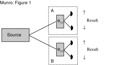
FIG. 1.: Schematic of a very generalized Bell experiment setup. After a source prepares two particles, these particles are directed out to the locations $A$ and $B$. At each location there is an analyzer with an adjustable parameters $\theta_{1,0},\theta_{2,0}$. The particles are then detected resulting in a binary result “$\uparrow$” or “$\downarrow$” individually.

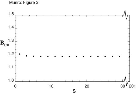
FIG. 2.: Plot of the ${B_{\rm CH}}$ versus s. A violation of the Bell inequality is possible for $|{B_{\rm CH}}|>1$.

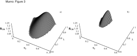
FIG. 3.: Plot of the ${B_{\rm CH}}$ versus $\psi$ and $\lambda$ for $s=3$ (Figure a) and $s=7$ (Figure b). A violation of the Bell inequality is possible for $|{B_{\rm CH}}|>1$.

- [1] Electronic address: billm@physics.uq.edu.au
- [2] J. S. Bell, Physics (N.Y.) 1, 195(1965).
- [3] J. F. Clauser,M. A. Horne, A. Shimony and R. A. Holt, Phys. Rev. Lett. 23, 880 (1969).
- [4] J. F. Clauser and M. A. Horne, Phys. Rev. D 10, 526(1974).
- [5] A. Einstein, B. Podolsky and N. Rosen, Phys. Rev. 47, 777 (1935).
- [6] It is well known that some weakly entangled systems do not violate a Bell inequality and yet can not be produced classically. However strongly entangled systems do generally violate the Bell inequalities and hence the Bell inequality is a method of characterising the entanglement in such cases.
- [7] P.G. Kwiat, P.H. Eberhard, A.M. Steinberg and R.Y. Chiao, Phys. Rev. A 49, 3209 (1994).
- [8] M. Freyberger, P.K. Aravind, M.A. Horne and A. Shimony, Phys. Rev. A 53, 1232 (1995).
- [9] E.S. Fry, T. Walther, and S. Li, Phys. Rev. A 52, 4381 (1996).
- [10] M. D. Reid, P. Deuar and W. J. Munro, accepted to Phys. Rev. A.
- [11] A. Gilchrist, P. Deuar and M. D. Reid , Phys. Rev. Lett. 80, 3169 (1998).
- [12] W.J. Munro, Phys. Rev. A. 59 4197 (1999).
- [13] W. J. Munro and G. J. Milburn, Phys. Rev. Lett. 81, 4285 (1998).
- [14] B. Yurke and D. Stoler, Phys. Rev. Lett. 79, 4941 (1997).
- [15] D.T. Smithey, M. Beck, M. Besley, and M.G. Raymer, Phys. Rev. Lett. 69, 2650 (1992).
- [16] N. D. Mermin, Phys. Rev. Lett. 65, 1838 (1990).
- [17] M. D. Reid, Phys. Rev. A 40, 913 (1989).
- [18] M. D. Reid and L. Krippner, Phys. Rev. A 47, 552 (1993).
- [19] C. W. Helstrom, Quantum Detection and Estimation Theory (Academic, New York, 1976).
- [20] A. S. Holevo, Probabilistic and Statistical Aspects of Quantum Theory (North–Holland, Amsterdam, 1982).
- [21] S.L.Braunstein , C.M. Caves and G.J.Milburn, ”Generalized uncertainty relations: Theory, examples and Lorentz Invariance”, Annals of Physics, 247, 135-173, number 1, (1996).
- [22] D. T. Pegg, and S. M. Barnett, Europhys. Lett.6, 483 (1988)
- [23] D. T. Pegg, and S. M. Barnett, Phys. Rev. A39, 1665 (1989)
- [24] Not all the inequalities used to test quantum mechanics require a binary choice. For example the Information theoretic Bell inequality requires a binary choice but the dimension of the subsystems is arbitrary.
- [25] S. L. Braunstein and C. M. Caves, Phys. Rev. Lett 61, 622 (1988).
- [26] W. J. Munro and M. D. Reid, Quantum Optics Letter 6, 1 (1994).
- [27] W. J. Munro and M. D. Reid, Phys Rev A 47, 4412 (1994).
- [28] W. J. Munro and M. D. Reid, Phys Rev A 50, 3661 (1994).