Quantum Stochastic Resonance in Electron Shelving

Abstract

Stochastic resonance shows that under some circumstances noise can enhance the response of a system to a periodic force. While this effect has been extensively investigated theoretically and demonstrated experimentally in classical systems, there is complete lack of experimental evidence within the purely quantum mechanical domain. Here we demonstrate that stochastic resonance can be exhibited in a single ion and would be experimentally observable using well mastered experimental techniques. We discuss the use of this scheme for the detection of the frequency difference of two lasers to demonstrate that stochastic resonance may have applications in precision measurements at the quantum limit.

Imagine that you are set the task of detecting a very weak periodic signal by means of its interaction with a suitable probe system. Given that the signal is weak, one intuitively may think that the optimal experimental set up should minimize any other interaction that the probe may undergo. However, this is not always the case and there are situations where noise can indeed play a constructive role in a high sensitivity detection. A clear illustration of this fact is provided by the phenomenon of stochastic resonance (SR) [1], where the response of a nonlinear system to external periodic driving is enhanced in the presence of noise. Typically [2], the signal-to-noise ratio (SNR) increases monotonically up to a maximum for certain optimal noise intensity, and then decreases gradually as randomization dominates over the cooperative effect between the coherent driving and the stochastic forces. The simplest system for describing the appearance of SR consists of a particle in a bistable potential subject to both thermal noise and a periodic forcing [3]. However, many other scenarios have been proposed and recent research has shown that SR may also be observed in some monostable systems [4]. Experimental research has confirmed that the phenomenon, if at first sight counter-intuitive, is rather ubiquitous. Since the first demonstration in a Schmitt trigger circuit [5], SR has been observed in a wide variety of physical systems, ranging from ring lasers to neuronal cells (see [6] for a detailed review). Moreover, there is experimental evidence that certain complex living systems (such as crickets) make use of SR to improve the sensitivity of their sensory organs [7].

Recently the concept of SR has been extended to the quantum domain [8, 9, 10]. However, experimental verifications at the level of individual quantum systems are difficult (see e.g. [11]) and it would be of great interest to find feasible experimental scenarios that allow the investigation of stochastic resonance in the quantum regime. In this letter we show that SR can be demonstrated in a conceptually simple truly microscopic quantum optical system. We first analyze the proposed system qualitatively, highlighting the key ideas behind our proposal and allowing for an intuitive understanding as to why SR arises in this scenario. Following this, we present a quantitative analysis of the phenomenon by means of exact numerical computation of the frequency response of the probe. We demonstrate that the SNR at the driving frequency is maximized at a certain noise level, an unambiguous signature of the occurrence of SR. Furthermore, to illustrate an application of SR in our proposed system, we discuss and simulate the noise-assisted precision measurement of the frequency difference of two coherent fields.

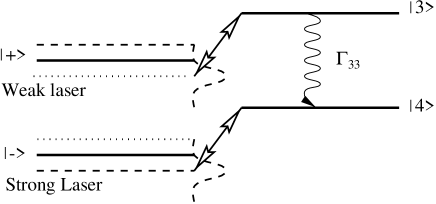
FIG. 1.: Four level system under coherent modulated driving with time-dependent Rabi frequency $\Omega$ giving rise to dressed states $|\pm\rangle$. Dashed (dotted) line gives position of dressed states for larger (smaller) value of $\Omega$. Transitions $-\leftrightarrow 3$ and $+\leftrightarrow 4$ are driven by broad band fields. The frequency distribution of the noisy fields is represented by the dashed curves. When the central frequency of each incoherent driving is tuned appropriately, the interaction can be made resonant with either the dressed level $\left|+\right\rangle$ or $\left|-\right\rangle$ depending on the value of $\Omega$ given by the modulation cycle (See text for details).

The scheme we present here is in principle easy to implement, as it relies entirely on techniques have been employed by experimentalists for more than 10 years. In Fig. 1 the system under consideration and the applied driving fields are shown. The probe consists of a four level atomic system subject to both coherent and incoherent radiation. The $1\leftrightarrow 2$ transition is driven by a resonant modulated coherent laser field of Rabi frequency $\Omega(t)$ while the $1\leftrightarrow 3$ and $2\leftrightarrow 4$ transitions are driven by noisy fields with effective pump rates $W_{33}$ and $W_{44}$ respectively. The atomic level $2$ can decay with a rate $2\Gamma_{22}$ and it is this radiation that will be detected. We assume that level $4$ is metastable and we neglect its spontaneous decay rate in the following. In addition, we assume that level $3$ can only decay, at a rate $2\Gamma_{33}$, into level $4$. The fact that the coherent driving is modulated implies that the Rabi frequency and therefore the energy separation $\hbar\Omega$ between the dressed levels $\left|\pm\right\rangle=1/\sqrt{2}(\left|1\right\rangle\pm\left|2\right\rangle)$ are time dependent. Let us consider the simplest case where the modulated driving can be described by a step function, as illustrated in Fig. 2. Then the time dependence of the coherent Rabi frequency is given by

$$\Omega(t)=\Omega\pm\Delta\Omega,$$ (1)

where $\Delta\Omega\ll\Omega$ (weak modulation), and where the $(+)$ sign holds for $t\in[kt_{m},(k+1/2)t_{m}]$, k is a positive integer, and the $(-)$ sign corresponds to the remaining part of the modulation cycle, $t_{m}$ denoting the corresponding modulation period. Under these conditions, the relative position of the dressed states alternates between two possible configurations, as illustrated by the dashed (dotted) lines in Fig. 1. For the sake of clarity, we will refer to these two possible situations as strong laser (i. e. larger Rabi frequency; larger energy separation between dressed levels) and weak laser (i. e. smaller Rabi frequency; smaller energy separation between dressed levels) regimes.

FIG. 2.: By means of suitably tuning the broad band fields driving the $1\leftrightarrow 3$ and $1\leftrightarrow 4$ transitions, the system may exhibit a bistable dynamics of bright and dark periods strongly synchronized with the modulation of the coherent driving.

We will now show in a qualitative way that the system we have described above may exhibit, when the broad band fields are suitably tuned, a dynamics of extended bright and dark periods in the resonance fluorescence intensity which are strongly synchronized with the modulated coherent driving field, as depicted in Fig. 2. However, synchronization is not the only signature of SR and we will show quantitatively later on that indeed the proposed scheme fulfills the necessary requirements for exhibiting SR.

Let us denote by $\hat{\omega}_{i}$, $(i=3,4)$, the central frequency of each broad band field, while $\omega_{i1}$ refers to the corresponding natural frequency of the atomic transition involved. Let us now choose the detunings $\Delta_{i1}=\hat{\omega}_{i}-\omega_{i1}$ as follows

$$\Delta_{31} = \frac{\Omega+\Delta\Omega}{2}$$ (2)

$$\Delta_{41} = -\,\frac{\Omega-\Delta\Omega}{2}\;.$$ (3)

This choice of detunings is schematically shown in Fig. 1. When the coherent driving operates in the weak mode, that is, when $\Omega(t)=\Omega-\Delta\Omega$, the noisy field driving the $1\leftrightarrow 3$ transition is resonant with the dressed level $\left|+\right\rangle$ while the field driving the $1\leftrightarrow 4$ is off-resonant. Under these circumstances, the system is rapidly pumped from $\left|1\right\rangle\leftrightarrow\left|3\right\rangle\leftrightarrow\left|4\right\rangle$. It remains in level 4 and as a consequence no light is emitted from the atom, i.e. we are in a dark period, given that level $\left|4\right\rangle$ is metastable. On the other hand, when the coherent driving is operating in the strong mode, the noise field driving the $1\leftrightarrow 4$ becomes resonant with the dressed level $\left|-\right\rangle$ while the driving $1\leftrightarrow 3$ becomes detuned. As a result, the system is pumped back and forth between level $\left|4\right\rangle$ and the dressed level $\left|-\right\rangle$, with photons being emitted at a rate proportional to $\Gamma_{22}/2$. Therefore, the system is in a bright period, i.e. the atom emits many photons. It can be understood quite easily how this synchronized dynamics depends on the noise intensity. If the effective pump rate $W_{ii}$, $(i=3,4)$, is too strong, e. g. $W_{ii}\gg\Delta\Omega$, the pump rates become insensitive to the value of $\Delta\Omega$, synchronization is lost and the observed fluorescence would just show a constant intensity. A lack of synchronization should also be observable in the opposite regime, where $W_{ii}$ is too weak, e. g. $W_{ii}<t_{m}^{-1}$, with the system exhibiting now extended bright and dark periods and an additional noise background in the fluorescence spectrum. Therefore, there seems to be an intermediate regime in which synchronization is optimal. We will demonstrate in the following that this optimal regime can be achieved and how in fact the system may exhibit stochastic resonance. To clearly identify SR we have to compute the autocorrelation function of the intensity emitted by the atom. We simplify it to a binary process, assuming value $1$ if the intensity exceeds a certain threshold (e.g. $10\%$ of the intensity expected in a bright period), and $0$ for intensities below the threshold. We then compute the power spectrum of this process which defines the spectral response of the system to a periodic perturbation. For that, we will have to compute explicitly the normalized spectrum and the corresponding SNR at the driving frequency. The starting point for evaluating these quantities is provided by the system’s master equation, whose relevant terms [12], under exact resonance for the $1\leftrightarrow 2$ transition, are as follow:

$${\dot{\rho}}_{++} = -(2W_{33}+\frac{\Gamma_{22}}{2})\rho_{++}+\frac{\Gamma_{22}}{2}\rho_{--}+2W_{33}\rho_{33}$$ (4)

$${\dot{\rho}}_{--} = \frac{\Gamma_{22}}{2}\rho{++}-(2W_{44}+\frac{\Gamma_{22}}{2})\rho_{--}+2W_{44}\rho_{44}$$ (5)

$${\dot{\rho}}_{+-} = \Gamma_{22}(\rho_{++}+\rho_{--})$$ (6)

$$- (W_{33}+W_{44}-\frac{3\Gamma_{22}}{2}+i\frac{\Omega}{2})\rho_{+-}-\frac{\Gamma_{22}}{2}\rho_{-+}$$ (7)

$${\dot{\rho}}_{33} = 2W_{33}\rho_{++}-(2W_{33}-2\Gamma_{33})\rho_{33}$$ (8)

$${\dot{\rho}}_{44} = =-{\dot{\rho}}_{++}-{\dot{\rho}}_{--}-{\dot{\rho}}_{33},\;\;{\dot{\rho}}_{-+}={\dot{\rho}}_{+-}^{*}$$ (9)

The last line arises from the preservation of trace and the hermiticity of the density operator. It should be stressed that this master equation is valid for a certain range of parameters in which the broadband assumption for the noise fields is correct, i.e. we can replace the effect of the noise by a simple pump rate $W_{ii}$. This approximation is valid if the frequency bandwidth $\Delta\omega_{i}$ $(i=3,4)$ of the noise field is larger than the spontaneous decay rates in the system and the detunings do not greatly exceed the bandwidth of the noise field. It should also be noted here that we are working in a dressed state picture, in which the incoherent pump rates are between the dressed level $|\pm\rangle$ and the level $3$ and $4$. This assumption is only valid if the Rabi frequency of the driving field on the $1\leftrightarrow 2$ transition is large compared to the bandwidth of the noise fields. This condition is intuitively clear, as in that case a noise field can selectively address only one dressed state. Therefore, our analysis applies provided that the following inequality holds

$$\Gamma_{ii}\ll\Delta\omega_{i}\ll\Omega,\,\,(i=3,4).$$ (10)

The master equation contains all the information about the dynamics of the system; however, if we are mainly interested in the behaviour of a single quantum system, e.g. a single ion in an ion trap, then it is more convenient to use the quantum jump approach ( see [13] and references therein). The main idea behind the quantum jump approach is to determine the time evolution of the system under the condition that no photon has been emitted on the $1\leftrightarrow 2$ transition. This conditional time evolution is no longer trace preserving and the decreasing trace reflects the probability that no photon has been emitted in the time interval $[0,t]$. The conditional time evolution can easily be obtained either directly from the master equation (removing some terms) or by rederiving it under the constraint that no photon has been emitted [13]. The key point is realizing that in order to obtain the conditional time evolution one has to remove from the ensemble all those systems that have emitted a photon. This can be done heuristically by removing the contribution $2\Gamma_{22}\rho_{22}$ from the time evolution equation for the population of the ground state $\rho_{11}$. When using dressed states $\left|\pm\right\rangle$, the result is that we need to replace Eqs. (4,5,7) by

$${\dot{\rho}}_{++} = -(2W_{33}+\Gamma_{22})\rho_{++}$$ (11)

$$+ \frac{\Gamma_{22}}{2}\rho_{+-}+\frac{\Gamma_{22}}{2}\rho_{-+}+2W_{33}\rho_{33}$$ (12)

$${\dot{\rho}}_{--} = -(2W_{44}+\Gamma_{22})\rho_{--}$$ (13)

$$+ \frac{\Gamma_{22}}{2}\rho_{+-}+\frac{\Gamma_{22}}{2}\rho_{-+}+2W_{44}\rho_{44}$$ (14)

$${\dot{\rho}}_{+-} = \frac{\Gamma_{22}}{2}(\rho_{++}+\rho_{--})$$ (15)

$$- (W_{33}+W_{44}+\Gamma_{22}+i\frac{\Omega}{2})\rho_{+-}$$ (16)

Given the conditional time evolution, the evaluation of the normalized power spectrum is a straightforward task. For the modulation described in Eq. (1) numerical results are presented in Fig. 3. This simulation shows the expected behaviour of a resonant-like process, with a sharp peak (a delta function within numerical precision) at the frequency of the modulation and subsequent weaker peaks at its odds harmonics. The peaks at even harmonics are suppressed due to the symmetry of the modulation. The emergence of delta peaks in the spectrum is a first indication of SR.

FIG. 3.: Numerical simulation of the power spectrum for a modulation as in Eq. (1). The other parameters are $\Omega=50\Gamma_{22},\Delta\Omega=10\Gamma_{22}$, $\Gamma_{33}=\Gamma_{22}$, $W_{33,weak}=0.0128$, $W_{33,strong}=W_{33,weak}/10$, and $W_{44,strong}=W_{33,weak}$, $W_{44,weak}=W_{33,strong}$ and detunings chosen as in Eqs. (2,3). The peaks are delta-functions to within the numerical precision. Harmonics at even multiples are suppressed because of the symmetry of the modulation.

In order to establish unambiguously the occurrence of SR, one has to evaluate the signal-to-noise ratio. This quantity, defined as the ratio of the spectral peak to the spectral background at a given frequency, is a measure of the probe sensitivity to the periodic driving. Fig. 4 shows the SNR at the modulation frequency, i.e. the frequency at which the power spectrum exhibits a delta peak. As expected, the SNR exhibits a maximum at an optimal noise pump rate. If the noise intensity is increased beyond this value, the sensitivity of the probe is diminished. Although we have presented numerical results for a specific choice of parameters, extensive numerical simulations show that SR can be observed over a wide range of parameters.

FIG. 4.: Output signal-to-noise (SNR) at the driving frequency as a function of the noise intensity. The parameters are chosen as in Fig. 3. The sharp rise of the noise intensity to a maximum for an intermediate value of the noise intensity followed by a slower fall-off towards smaller SNR is a clear signature of the occurrence of SR.

The scheme discussed above may seem academic, but it allows us to exemplify how stochastic resonance could be observed at the level of a single quantum system using currently available experimental techniques. Moreover, we will now show that this phenomenon may find practical applications in precision measurements. To this end

FIG. 5.: Output signal-to-noise (SNR) at the driving frequency as a function of the noise intensity for the two beating lasers driving the $1\leftrightarrow 2$ transition. The parameters are $\Omega_{1}=50\Gamma_{22},\Omega_{2}=10\Gamma_{22}$, $\Gamma_{33}=\Gamma_{22}$ and the detuning between the lasers is chosen to be $\delta\omega=0.049\Gamma_{22}$. For the noise fields we choose $W_{33,max}=W_{44,max}$ and detunings as in Eqs. (2,3). The bandwidth of the noise fields are equal and chosen to be $6.66\Gamma_{22}$. The sharp rise to a maximum for an intermediate value of the noise intensity followed by a slower fall-off towards smaller SNR where randomization dominates is a signature of the occurrence of SR.

we will discuss how the sensitivity for the detection of a frequency mismatch between two coherent fields can be enhanced using incoherent driving, i.e., employing SR.

Let us consider two coherent fields with Rabi frequencies $\Omega_{1}$ and $\Omega_{2}$, whose oscillation frequencies differ by a small amount $\delta\omega$. As it is well known, the superposition of two laser fields in a running wave configuration results in a beating signal. The idea is to use this modulated signal as our driving field (giving rise to the dressed states $|\pm\rangle$) while tuning appropriately the additional incoherent driving fields (see Fig. 1 for illustration). Numerical simulations of the power spectrum for experimentally accessible parameters reveal again that the frequency response of the atomic system exhibits stochastic resonance. The signal to noise ratio for the first delta peak in the power spectrum is shown in Fig. 5. The optimal performance, that is, the largest SNR, is achieved for certain finite but non-zero noise intensity. This result implies that stochastic resonance can have applications for example in frequency measurements.

Summarizing, we have showed that the phenomenon of SR, a paradigm of the counter-intuitive role that noise may play in high sensitivity detection, can be demonstrated at the level of a single ion. As an illustration of the potential that this effect may have, we have discussed the use of a SR scheme for the detection of the frequency difference of two lasers. As the proposed experimental scenario relies on techniques well mastered by quantum opticians, quantum SR may be expected to open up new experimental possibilities in precision measurements at the quantum limit.

This work was supported by The Leverhulme Trust, the UK EPSRC and the European Union. We would also like to thank D.M. Segal and R.C. Thompson and their experimental ion trapping group at Imperial College for interesting discussions and P.L. Knight for helpful comments on the manuscript.

REFERENCES

- [1] R. Benzi et al, J. Phys. A 14, L453 (1981).
- [2] There exist a class of systems for which the SNR may display a multiplicity of maxima, as described by J. M. G. Vilar and J. M. Rubí, Phys. Rev. Lett. 78, 2882 (1997).
- [3] B. McNamara and K. Wiesenfeld, Phys. Rev. A 39, 4854 (1989); K. Wiesenfeld and F. Moss, Nature 373, 33 (1995).
- [4] J. M. G. Vilar and J. M. Rubí, Phys. Rev. Lett. 77, 2863 (1996).
- [5] S. Fauve and F. Heslot, Phys. Lett. 97A, 5 (1983).
- [6] L. Gammaitoni, P. Hänggi, P. Jung, and F. Marchesoni, Rev. Mod. Phys. 70, 223 (1998) and references therein.
- [7] J. E. Levin and J. P. Miller, Nature 380, 165 (1996).
- [8] R. Löfstedt and S.N. Coppersmith, Phys. Rev. Lett. 72, 1947 (1994).
- [9] D.O. Reale, A.K. Pattanayak, and W.C. Schieve, Phys. Rev. E 51, 2925 (1995).
- [10] M. Grifoni and P. Hänggi, Phys. Rev. Lett. 76, 1611 (1996).
- [11] A. Buchleitner and R.N. Mantegna, Phys. Rev. Lett. 80, 3932 (1998); T. Wellens and A. Buchleitner, J. Phys. A. 32, 2895 (1999).
- [12] The temporal evolution for the crossed coherences turns out to be ruled by decoupled differential equations. If initially present, these terms simply get exponentially damped. Note that, as opposed to the coherence terms between the dressed levels, the crossed coherences are not re-populated after an emission process.
- [13] M.B. Plenio and P.L. Knight, Rev. Mod. Phys. 70, 101 (1998).