Stochastic Resonance and Nonlinear Response by NMR Spectroscopy

Abstract

We revisit the phenomenon of quantum stochastic resonance in the regime of validity of the Bloch equations. We find that a stochastic resonance behavior in the steady-state response of the system is present whenever the noise-induced relaxation dynamics can be characterized via a single relaxation time scale. The picture is validated by a simple nuclear magnetic resonance experiment in water.

The interplay between dissipation and coherent driving in the presence of dynamical nonlinearities gives rise to a variety of intriguing behaviors. The most paradigmatic and counterintuitive example is the phenomenon of stochastic resonance (SR), whereby the response of the system to the driving input signal attains a maximum at an optimum noise level [1]. By now, stochastic resonance has been demonstrated in several overdamped bistable systems as diverse as lasers, semiconductor devices, SQUID’s, and sensory neurons, the required noise tuning being accomplished by either controlling the injection of external noise or by suitably varying the temperature of the noise-inducing environment.

Due to the broad typology of situations it can exemplify and its inherent simplicity, a preferred candidate for theoretical analysis is represented by a driven dissipative two-level system (TLS). The investigation has only recently been taken into the quantum world, where some prominent results have been established for the so-called spin-boson model. The latter schematizes the archetypal situation of a driven quantum-mechanical tunneling system in contact with a harmonic heat bath, the resulting dissipation being commonly addressed in the linear Ohmic regime [2, 3, 4, 5, 6]. Within this framework, a quantum SR phenomenon induced by a resonant irradiation with a continuous-wave field has been characterized analytically [3, 5] and verified through exact numerical path-integral calculations [3, 6].

In the present work, we show that a stochastic resonance phenomenon occurs for a much wider class of driven two-state quantum systems, whose relaxation dynamics can be accounted for by conventional Bloch equations. We find that, irrespective of the details of the microscopic picture, the essential requirement is the emergence of a single relaxation time scale. The prediction is neatly demonstrated by a nuclear magnetic resonance experiment on a water sample.

Let us consider a two-state quantum system whose density operator $\rho$ is represented in terms of the Bloch vector $\vec{s}$ as $\rho=(1+\vec{s}\cdot\vec{\sigma})/2$ i.e., $s_{i}(t)=\langle\sigma_{i}(t)\rangle$, $i=1,2,3$, in the customary pseudo-spin formalism [7]. Within the semigroup approach for open quantum systems [8], the most general (completely) positive relaxation dynamics induced by the coupling to some environment is described by a quantum Markov master equation of the form

$$\dot{\rho}=-{i\over\hbar}[H(t),\rho]+{1\over 2}\sum_{k,l=1}^{3}a_{kl}\left\{[\sigma_{k}\rho,\sigma_{l}]+[\sigma_{k},\rho\sigma_{l}]\right\}\,.$$ (1)

The Hamiltonian $H(t)$, which describes the interaction of the TLS with the (classical) driving field, can be expressed as $H(t)={\hbar\omega_{0}}\sigma_{3}/2+V(t)$, $V(t)={\hbar(2\omega_{1})}\cos(\Omega t)\sigma_{1}/2$, where the Larmor frequency $\omega_{0}=(E_{2}-E_{1})/\hbar$ associated with the TLS energy splitting and the Rabi frequency $\omega_{1}$ proportional to the alternating field amplitude have been introduced. The above Hamiltonian is identical to the one describing a driven tunneling process in a symmetric double-well system with “localized” states provided by $\sigma_{1}$-eigenstates: By rotating the spin coordinate by $\pi/2$ about the $\hat{y}$-axis, one formally recovers the picture of tunneling in the $\hat{z}$-representation that is encountered in the literature [1, 2, 3, 4, 5, 6, 10]. The dissipative component of the TLS dynamics is fully characterized by the positive-definite $3\times 3$ relaxation matrix $A=\{a_{kl}\}$, determining the equilibrium state of the system and the relaxation time scales connected with the equilibration process. The Bloch equations correspond to an especially simple realization of $A$, the non-zero elements being specified in terms of 3 independent parameters: $a_{11}=a_{22}=(2T_{1})^{-1}$, $a_{33}=(T_{2})^{-1}-(2T_{1})^{-1}$, $a_{12}=a_{21}^{\ast}=i(\sqrt{2}T_{1})^{-1}s_{eq}$. $T_{1},T_{2}$, and $s_{eq}$ are identified as the longitudinal and transverse lifetimes, and the equilibrium value of the population difference respectively. Thus, Eq. (1) takes the following familiar form [9]:

$$\left\{\begin{array}[]{lll}\dot{s_{1}}&=&\;\;\>\omega_{0}s_{2}-T_{2}^{-1}s_{1}\>,\\ \dot{s}_{2}&=&-\omega_{0}s_{1}-T_{2}^{-1}s_{2}+2\omega_{1}\cos(\Omega t)s_{3}\>,\\ \dot{s}_{3}&=&-2\omega_{1}\cos(\Omega t)s_{2}-T_{1}^{-1}(s_{3}-s_{eq})\>.\end{array}\right.$$ (5)

In microscopic derivations of (5), including the ones based on the spin-boson model in the appropriate limit [10, 5], relaxation is caused by elementary processes involving noise-assisted transitions between the TLS energy levels or purely dephasing events with no energy exchange between the system and the environment. The overall relaxation rates $T_{1,2}^{-1}$ are obtained by integrating such fluctuation and dissipation effects over the environmental modes, weighted by the appropriate noise spectral densities. Since the latter contain the coupling strength between the system and the environment, relaxation rates are themselves directly proportional to the underlying noise intensity. Note that the above treatment in terms of a constant matrix $A$ is only valid for external fields that are relatively weak on the TLS energy scale i.e., $2|\omega_{1}|\ll\omega_{0}$. In spite of the many restrictions involved, it is remarkable that the Bloch equations (5) are of such a wide applicability to cover the majority of magnetic or optical resonance experiments.

For times long compared to the time scales $T_{1,2}$ of the transient dynamics, the motion of the system reaches a steady-state behavior that is insensitive to the initial condition and acquires the periodicity of the driving. In particular, the asymptotic TLS coherence properties are captured by the off-diagonal matrix element $s_{1}(t)$, $s_{2}(t)$. It is standard practice to formulate an input/output problem, where the TLS is regarded as a dynamical system generating $s_{1}(t)=\langle\sigma_{1}(t)\rangle$ as the output signal in response to a given input drive $V(t)$. By letting $\lim_{t\rightarrow\infty}\langle\sigma_{1}(t)\rangle=s_{1}^{\infty}(t)$ denote the limiting steady-state value of $s_{1}(t)$, a figure of merit for the system response is the so-called fundamental spectral amplitude [1],

$$\eta(\Omega,\omega_{1})=|s_{1}^{\infty}(t)|=\hbar(2\omega_{1})|\chi(\Omega,\omega_{1})|\>,$$ (6)

where the connection to the complex susceptibility $\chi(\Omega,\omega_{1})=\chi^{\prime}(\Omega,\omega_{1})-i\chi^{\prime\prime}(\Omega,\omega_{1})$ is made explicit.

The competition between driving and dissipative forces sets the boundary between the linear vs. nonlinear response regimes. In the limit where $\omega_{1}\ll T_{1,2}^{-1}$, only first-order contributions in $\omega_{1}$ are significant and the susceptibility $\chi(\Omega,\omega_{1})=\chi(\Omega)$ in (6) can be calculated within ordinary linear response theory. The linear regime implies that absorption of energy from the applied field occurs without disturbing populations from their equilibrium value $s_{eq}$. Linear behavior breaks down whenever $\omega_{1}\gtrsim T_{1,2}^{-1}$. Strongly nonlinear-response regimes can be entered for arbitrarily weak fields as long as the coupling to the environment and the induced noise effects are weak enough. For both linear and nonlinear driving, the amplitude $\eta(\Omega,\omega_{1})$ of the output signal also depends on the various parameters characterizing the noise process. Quite generally, the phenomenon of stochastic resonance can be associated with the appearance of non-monotonic dependencies upon noise parameters, leading to the optimization of the response at a finite noise level.

We focus on the Bloch equations (5) with resonant driving, $\Omega=\omega_{0}$. It is then legitimate to invoke the rotating-wave approximation and replace the alternating field $V(t)$ with $V(t)=\hbar\omega_{1}\cos(\Omega t)\sigma_{1}/2-\hbar\omega_{1}\sin(\Omega t)\sigma_{2}/2$. The rotating-frame description of the Bloch vector $\vec{\mu}$ is introduced via the time-dependent rotation $R=\exp(i\Omega\sigma_{3}t/2)$ i.e., $\rho_{R}=R\,\rho\,R^{-1}=(1+\vec{\mu}\cdot\vec{\sigma})/2$, $\vec{\mu}=(u,v,w)$ [7]. The steady-state solution to the Bloch equations is well known [11, 12]. In particular, $\chi^{\prime}$ and $\chi^{\prime\prime}$ are read from the dispersive and absorptive components $u,v$ of the Bloch vector respectively, and the spectral amplitude $\eta(\Omega=\omega_{0},\omega_{1})=(u^{2}+v^{2})^{1/2}$. A simple expression is found for the nonlinear response:

$$\eta(\Omega=\omega_{0},\omega_{1})=s_{eq}\,\frac{\omega_{1}T_{2}}{1+\omega_{1}^{2}T_{1}T_{2}}\>.$$ (7)

Suppose now that we have the capability of manipulating the strength of the coupling of the TLS to its environment, thereby changing the relaxation times $T_{1},T_{2}$. For a fixed driving amplitude $\omega_{1}$, $\eta$ displays purely monotonic behaviors if $T_{1},T_{2}$ are varied independently. However, if a single relaxation time is present, $T_{1}=T_{2}=T_{12}$, $\eta$ develops a local maximum characterized by

$$T_{12}^{\ast}=\omega_{1}^{-1}\>,\hskip 14.22636pt\eta(\Omega=\omega_{0},\omega_{1},T_{12}^{\ast})={s_{eq}\over 2}\>.$$ (8)

The occurrence of such a peak in the steady-state response as a function of the noise strength can be pictured as a stochastic resonance effect in the TLS. Physically, the condition for the maximum in (8) can be thought of as a synchronization between the periodicity of the rotating-frame vector in the absence of relaxation and the additional time scale emerging when dissipation is present. In semiclassical terms, a constraint of the form $T_{1}=kT_{2}$, $k=$ const., indicates that the spectral densities of the fluctuating environmental fields along different directions are not independent upon each other. Simple examples include noise processes that effectively originate from a single direction or that equally affect the system in the three directions. In fact, the existence of a single relaxation time is a feature shared with earlier investigations of quantum SR based on the driven spin-boson model [3, 5], where it arises as a necessary consequence of the initial assumption that environmental forces exclusively act along the tunneling axis. However, we emphasize that our discussion is done without reference to a specific model, encompassing in principle a larger variety of physical situations.

Apart from this conceptual difference, the SR phenomenon evidenced above is characterized by the same distinctive features found for the spin-boson model on resonance [3, 5]. According to (8), the maximum steady-state response is independent of the driving amplitude, whereas the position of the peak shifts toward shorter relaxation times with increasing $\omega_{1}$. Thus, weaker noise strengths require weaker input fields to attain a large response. This brings the nonlinear nature of the SR mechanism to light, for weaker dissipation more easily pushes the system into a regime where $\omega_{1}T_{12}\gtrsim 1$. No SR peak occurs in the limit $\omega_{1}T_{12}\ll 1$ where linear response theory applies and $\eta\rightarrow s_{eq}(\omega_{1}T_{12})\ll s_{eq}$. Thus, SR results in efficient noise-assisted signal amplification. Breakdown of linear behavior is more convincingly demonstrated by looking at the dependence of the response (7) upon the external field strength. It is easily checked that the condition (8) simultaneously optimizes the response against $\omega_{1}$, with $\omega_{1}^{\ast}=(T_{1}T_{2})^{-1/2}$. However, it is only when $T_{1}=kT_{2}$ that the existence of such an optimal field amplitude coexists with a SR effect.

Nuclear Magnetic Resonance (NMR) provides a natural candidate for a direct experimental verification of the predicted phenomenon. In NMR, the Bloch equations (5) describe the motion of the magnetization vector $\vec{M}$ of spin 1/2 nuclei (¹H) that are subjected to a static magnetic field $B_{0}$ along the $\hat{z}$-axis and a radio-frequency signal with amplitude $2|B_{1}|\ll B_{0}$ applied at frequency $\Omega$ along the $\hat{x}$-axis. The mapping is established by identifying $\vec{s}=\vec{M}$, $s_{eq}=M_{0}$, $\omega_{0}=\gamma B_{0}$, $\omega_{1}=\gamma B_{1}$, $M_{0}$ and $\gamma$ denoting the equilibrium magnetization and the gyromagnetic ratio respectively. Relaxation processes arise due to a multiplicity of microscopic mechanisms [12]. For a liquid spin $1/2$ sample, the leading contribution arises from fluctuations of the local dipolar field caused by bodily motion of the nuclei. The longitudinal relaxation time $T_{1}$ is essentially determined by the $\hat{x}$- and $\hat{y}$- components of the local magnetic fields at the Larmor frequency, while the transverse lifetime $T_{2}$ takes extra contributions from static components of the $\hat{z}$-field, implying that $T_{2}\leq 2T_{1}$ ordinarily [12, 13]. Let us assume as above that $\Omega=\omega_{0}$. Once the steady state is reached, the magnetization vector $\vec{M}$ precesses about the $\hat{z}$-axis with the periodicity of the r.f. field. The variation of the dipole moment in the tranverse plane induces a measurable e.m.f. in a Faraday coil. This provides access to the relevant quantity $\eta$ of Eqs. (6)-(7), which represents the length of the transverse magnetization vector, $(u^{2}+v^{2})^{1/2}=(M_{x}^{2}(t)+M_{y}^{2}(t))^{1/2}$.

Our experiment consists in probing the steady-state magnetization response of water as a function of the noise strength inducing the natural relaxation processes. The ¹H Larmor frequency at $B_{0}=9.4$ T is $\omega_{0}/2\pi=400$ MHz, with relaxation times $T_{1}=3.6$ s, $T_{2}=2.5$ s. The sample can be brought to a regime where $T_{1}\simeq T_{2}$ upon addition of the paramagnetic salt copper sulfate (CuSO₄). With concentrations in the range between 40 mM and 100 mM, collision events with the impurity dominate the nuclear relaxation dynamics. This effectively pushes the system into a regime of rapid motion where the correlation time of the local magnetic fields seen by the nuclei is very short on the scale $\omega_{0}^{-1}$, thereby ensuring that $T_{1}=T_{2}=T_{12}$ [13]. Higher concentrations of the CuSO₄ additive result in a shorter relaxation time $T_{12}$ hence implying an effective tuning of the noise strength. All measurements were performed at room temperature with a Bruker AMX400 spectrometer on five water samples with additive concentration in the above range.

Independent measurements of $T_{1}$ and $T_{2}$ were made to confirm that the amount of CuSO₄ was sufficient to make them equal. $T_{1}$ was measured via an inversion recovery technique [13], by looking at the recovery curve of $M_{z}(t)$ after the application of a $\pi$ pulse causing $M_{z}(0)=-M_{0}$. Values of $T_{2}$ were inferred from the decay of the echo signals in a standard Carr-Purcell sequence where $\pi$ rotations were used to refocus dephasing due to inhomogeneous broadening [13]. For the 5 concentrations utilized, $T_{1}$ and $T_{2}$ were found to be within 1 ms of the average value $T_{12}$ which is listed for each sample in Table I.

CuSO4 (mM)	$T_{12}$ (ms) $\pm$ 1 ms
40	45.5
50	36.5
60	28.5
75	25.0
100	18.0

TABLE I. Relaxation time $T_{12}=T_{1}=T_{2}$ as a function of the CuSO₄ paramagnetic impurity concentration for the 5 water samples used in the experiment.

For each sample, the response to a long external r.f. pulse was measured for various values of the driving amplitude. For a given driving amplitude, the duration of the pulse was increased up to about 200 ms and the reading was continued until a constant e.m.f. value was reached, confirming that all transient responses had sufficiently decayed. Under these conditions, the observed steady-state value is equivalent to the one produced by a cw-irradiation as assumed in Eqs. (5). A delay long with respect to $T_{12}$ was waited between each pulse to allow the sample to return to equilibrium. The value of the r.f. amplitude was determined by extrapolating measurements of the nutation rate $\nu_{1}=\omega_{1}/2\pi$ at a high field setting down to the relevant lower-field domain in the neighbourhood of $\omega_{1}\approx T_{12}^{-1}$. While the relative error between two r.f. setting is found to be small, the systematic error associated with the extrapolation turns out to be significant. A linear correction of the frequency scale was included in the analysis to compensate for such error.

The experimental results are shown in Figs. 1 and 2. Fig. 1 evidences the SR peak for three values of the driving amplitude. A bell-shaped maximum in the response profile is clearly visible, as well as the expected shifting of the peak location with increasing $\omega_{1}$. For each curve, the SR condition $T_{12}^{\ast}\approx\omega_{1}^{-1}$ of Eq. (8) is in fairly good agreement with the observed behavior, existing discrepancies being accounted for by the residual error affecting the determination of $\omega_{1}$. In Fig. 2 the complementary characterization of the SR effect in terms of nonlinear response to the driving field is displayed for three values of $T_{12}$. In each case, ordinary linear response theory is valid for small $\omega_{1}$ to the left side of the maximum. Thus, SR reveals itself as a signal optimization marking the crossover between linear and nonlinear response.

Beside validating the predictions from the Bloch equations (5), our experimental results also support the conclusions independently reached in earlier theoretical analyses [3, 5]. A few remarks are in order concerning the specific case of NMR. First, the present experiment is not a stochastic NMR experiment [14]. While the obvious similarity is that both methods probe the nuclear spin system by looking at the transverse magnetization response, in stochastic NMR the system is directly excited by noise, which is therefore always extrinsic (and classical) in origin. More importantly, as mentioned already, the solutions to the Bloch equation have a long history as a tool to investigate magnetic resonance behaviors. In particular, the existence of an optimum r.f. amplitude $\omega_{1}^{\ast}=(T_{1}T_{2})^{-1/2}$ is a feature pointed out long ago by Bloch himself [9]. However, only the SR paradigm provides the motivation to regard relaxation features as controllable output parameters and to look at the usual response behavior along different axes in the parameter space. Even once this is done, this does not automatically lead to SR. Rather, it is the recognition that a single axis $T_{1}=T_{2}$ is effectively needed to bring out the fingerprint of the phenomenon and the novel element added to the standard NMR analysis.

In summary, we established both theoretically and experimentally the occurrence of stochastic resonance in two-state quantum systems whose relaxation dynamics are described by Bloch equations. In addition to substantially broadening the existing paradigm for stochastic resonance in quantum systems, our results point to the possibility of characterizing intrinsic relaxation behavior via resonance effects. By offering an optimized way for input/output transmission against noise, stochastic resonance carries a great potential for systems configured to perform specific signal processing and communication tasks [1]. In particular, full exploitation of stochastic resonance phenomena could potentially disclose a useful scenario for reliable transmission of quantum information in the presence of environmental noise and decoherence.

This work was supported by the U.S. Army Research Office under grant number DAAG 55-97-1-0342 from the DARPA Microsystems Technology Office.

^† Corresponding author: vlorenza@mit.edu

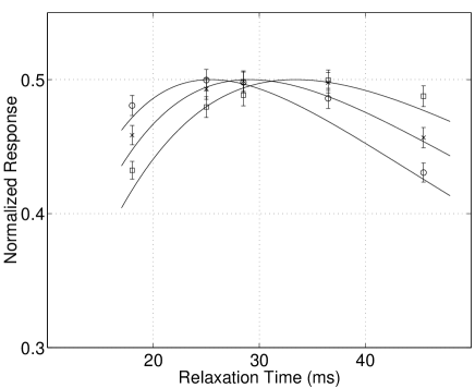
FIG. 1.: Normalized steady-state response $\eta/s_{eq}$ vs. relaxation time $T_{12}$ for resonant driving $\Omega/2\pi=400$ MHz at different driving amplitudes: $\omega_{1}/2\pi$= 6.3 Hz (circles), 5.5 Hz (crosses), 4.8 Hz (squares). Solid lines: theoretical predictions from Eq. (4), after systematic correction for the frequency (no free parameters).

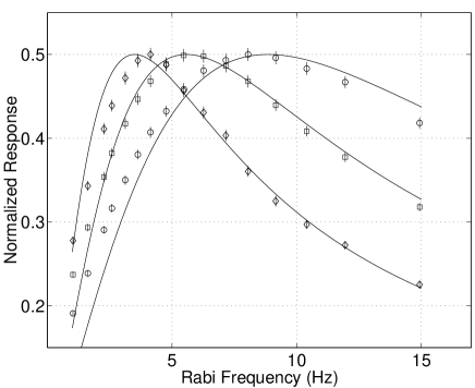
FIG. 2.: Normalized steady-state response $\eta/s_{eq}$ vs. Rabi frequency $\omega_{1}/2\pi$ for resonant driving $\Omega/2\pi=400$ MHz at different relaxation times: $T_{12}$= 18.0 ms (circles), 28.5 ms (squares), 45.5 ms (diamonds). Solid lines as above.

REFERENCES

- [1] For a comprehensive review, see L. Gammaitoni et al., Rev. Mod. Phys. 70, 223 (1998).
- [2] R. Löfstedt and S. N. Coppersmith, Phys. Rev. Lett. 72, 1947 (1994); Phys. Rev. E 49, 4821 (1994).
- [3] D. E. Makarov and N. Makri, Phys. Rev. B 52, R2257 (1995); Phys. Rev. E 52, 5863 (1995).
- [4] M. Grifoni and P. Hänggi, Phys. Rev. Lett. 76, 1611 (1996); Phys. Rev. E 54, 1390 (1996).
- [5] T. P. Pareek, M. C. Mahato, and A. M. Jayannavar, Phys. Rev. B 55, 9318 (1997).
- [6] M. Thorwart et al., Chem. Phys. 235, 61 (1998).
- [7] L. Allen and J. H. Eberly, Optical Resonance and Two-Level Systems (Dover, New York, 1975).
- [8] R. Alicki and K. Lendi, Quantum Dynamical Semigroups and Applications (Springer-Verlag, Berlin, 1987).
- [9] F. Bloch, Phys. Rev. 70, 460 (1946).
- [10] A. Leggett et al., Rev. Mod. Phys. 59, 1 (1987).
- [11] H. C. Torrey, Phys. Rev. 76, 1059 (1949).
- [12] A. Abragam, Principles of Nuclear Magnetism (Oxford University Press, New York, 1961).
- [13] C. P. Slichter, Principles of Magnetic Resonance (Sprin- ger, Berlin, 1990).
- [14] B. Blumich and D. Ziessow, J. Magn. Res. 52, 42 (1983); B. Blumich and R. Kaiser, ibid. 54, 486 (1983).