Local symmetry properties of pure 3-qubit states.

Abstract

Entanglement types of pure states of three spin-$\tfrac{1}{2}$ particles are classified by means of their stabilisers in the group of local unitary transformations. It is shown that the stabiliser is generically discrete, and that a larger stabiliser indicates a stationary value for some local invariant. We describe all the exceptional states with enlarged stabilisers.

1 Introduction

It is only relatively recently that the importance of entanglement has been fully realised. Not only, as Schrödinger emphasised [1], does it constitute one of the chief differences between classical and quantum mechanics, and the main obstacle to an intuitive understanding of quantum mechanics; the recent discovery is that it is also a resource, yielding much greater capabilities than classical physics in information processing and communication (see for example [2]).

It is therefore important to analyse and measure this resource. A full analysis has so far been achieved only for pure state systems with two component parts [3, 4]; for multipartite systems there are several different possible measures of entanglement [5, 6, 8, 9, 10, 11], the relation between them being incompletely understood. A full quantitative analysis of entanglement even for pure states of three-part systems appears to be difficult (but see [9]). Our aim in this paper is to give a qualitative analysis of the entanglement of such states, using group-theoretic methods to classify the possible kinds of entanglement.

The nature of the entanglement between the parts of a composite system should not depend on the labelling of the basis states of each of the part-systems; it is therefore invariant under unitary transformations of the individual state spaces. Such transformations are referred to as local unitary transformations, though there is no implication that the part-systems should be spatially separated. If the part-systems have individual state spaces $\mathcal{H}_{1},\ldots,\mathcal{H}_{n},$ so that the space of pure states of the composite system is $\mathcal{H}_{1}\otimes\ldots\otimes\mathcal{H}_{n},$ then a local unitary transformation is of the form $U_{1}\otimes...\otimes U_{n}$ where $U_{i}$ is a unitary operator on $\mathcal{H}_{i}.$ The set of all such transformations is a group $G,$ whose orbits in $\mathcal{H}_{1}\otimes...\otimes\mathcal{H}_{n}$ are equivalence classes of states with the same entanglement properties. Each orbit therefore corresponds to a complete specification of entanglement. The orbits can be classified by their dimensions, which are determined by the stabiliser subgroups of points on the orbit; the relation is

$$\text{dim}\mathcal{O}+\text{dim}\mathcal{S}=\text{dim}G$$ (1)

where $\mathcal{O}$ is an orbit and $\mathcal{S}$ is the stabiliser of any point on $\mathcal{O},$ i.e. the set of elements of $G$ which leave a point unchanged (different points on the same orbit have conjugate stabilisers, which have the same dimension).

This paper is concerned with pure states of three spin-$\tfrac{1}{2}$ particles $(n=3;$ $\mathcal{H}_{1}=\mathcal{H}_{2}=\mathcal{H}_{3}=\mathbb{C}^{2}.)$ We will show that for most states (all but a set of lower dimension) the stabiliser is discrete, so the dimension of the orbit is the same as that of the group $G.$ Classifying types of entanglement by the dimension of the orbit is therefore equivalent to identifying certain exceptional types of entanglement, which can be expected to be particularly interesting and important. One way in which this manifests itself is that any such exceptional entanglement is necessarily associated with an extreme value of one of the local invariants which form coordinates in the space of entanglement types, and from which any measure of entanglement must be constructed.

The organisation of the paper is as follows. In Section 2 we review the case of two spin-$\tfrac{1}{2}$ particles. The results here are well-known, but we include them for the sake of completeness and orientation. In Section 3 we prove the general theorem about three spin-$\tfrac{1}{2}$ particles mentioned in the preceding paragraph. Section 4 consists of the theorem concerning the association between enlarged stabilisers and stationary values of invariants. Section 5 contains the classification of exceptional entanglement types in the system of three spin-$\tfrac{1}{2}$ particles, in which we examine all the states which are identified as non-generic in the theorem of Section 3. Section 6 is a summary listing these exceptional states. They are illustrated by means of plots of their two-particle entanglement entropies in an appendix.

Acknowledgments

We are indebted to Dr. Ian McIntosh for a helpful conversation, and to Prof. A. Popov for drawing reference [12] to our attention.

The research of the first author was supported by the EPSRC.

2 The Stabiliser for the 2-particle case.

A pure state of two spin-$\tfrac{1}{2}$ particles can be written as

$$|\Psi\rangle=\sum_{i}t_{ij}|\psi_{i}\rangle|\psi_{j}\rangle$$ (2)

where $\{|\psi_{1}\rangle,|\psi_{2}\rangle\}$ is a basis of one-particle states. Having fixed this basis, we can identify the state $|\Psi\rangle$ with the matrix of coefficients $T=(t_{ij}).$ The group of local transformations is

$$G_{2}=U(1)\times SU(2)\times SU(2),$$ (3)

since the phases in the individual unitary transformations can be collected together. The effect of a local transformation $(e^{i\theta},X,Y)$ on $T$ is to change it to $e^{i\theta}XTY^{\mathrm{T}},$ so the condition for $(e^{i\theta},X,Y)$ to belong to the stabiliser of $|\Psi\rangle$ is

$$T=e^{i\theta}XTY^{\mathrm{T}}.$$ (4)

For a 2-particle state, we can always perform a Schmidt decomposition, so we need only consider states for which

$$T=\begin{pmatrix}p&0\\ 0&q\end{pmatrix},$$

i.e.

$$|\Psi\rangle=p|\uparrow\rangle|\uparrow\rangle+q|\downarrow\rangle|\downarrow\rangle$$

where $p,q$ are real and positive. Multiplying the stabiliser equation on the right by $\overline{Y},$ where the overbar denotes complex conjugation, and writing

$$X=\begin{pmatrix}r&s\\ -\overline{s}&\overline{r}\end{pmatrix},\quad Y=\begin{pmatrix}g&h\\ -\overline{h}&\overline{g}\end{pmatrix},$$ (5)

we obtain:

$$\begin{pmatrix}p&0\\ 0&q\end{pmatrix}\begin{pmatrix}\overline{r}&\overline{s}\\ -s&r\end{pmatrix}=e^{i\varphi}\begin{pmatrix}g&h\\ -\overline{h}&\overline{g}\end{pmatrix}\begin{pmatrix}p&0\\ 0&q\end{pmatrix}.$$

For given $p,q,$ we want to find the set of solutions $(\varphi,g,h,r,s)$ with $\varphi$ real and $g,h,r,s\in\mathbb{C},$ with $|g|^{2}+|h|^{2}=1,|r|^{2}+|s|^{2}=1.$ If $p\neq 0$, then $g=\overline{r}e^{-i\varphi}$. If $q\neq 0$, then $\overline{g}=re^{-i\varphi}$. Therefore either $r=0$ or $\varphi=n\pi$. Also

$$h=\frac{p}{q}\overline{s}e^{-i\varphi}=\frac{q}{p}\overline{s}e^{i\varphi}$$

So unless $p=q$ (since $p$ and $q$ were obtained by a Schmidt decomposition, they cannot be negative) we must have $\frac{p}{q}e^{-i\varphi}-\frac{q}{p}e^{i\varphi}\neq 0$ and so $s=0$. The states now fall naturally into three classes:

Case 1: The General case.

If $p\neq 0$ and $q\neq 0$ and $p\neq q$ then $s=h=0$ and $e^{i\varphi}=e^{-i\varphi}=\pm 1$ so we can absorb that external sign into $X.$ This is the subgroup

$$\varphi=0,\quad X=e^{i\nu\sigma_{z}},\quad\quad\quad Y=\bar{X}.$$ (6)

The stabiliser has one parameter, $\nu$.

Case 2: The Unentangled case.

Without loss of generality, we can take $p=1$, $q=0$. Putting $g=e^{i\theta}$, this is the subgroup

$$(e^{i\varphi},g,r)=(e^{i\varphi},e^{i\theta},e^{-i(\varphi+\theta)})$$ (7)

The stabiliser has two parameters, $\varphi$ and $\theta$.

Case 3: The Maximally Entangled Case.

This occurs when $p=q=1/\sqrt{2}$. Then

$$g =\overline{r}e^{-i\varphi}=\overline{r}e^{i\varphi}$$

$$h =-se^{-i\varphi}=-se^{i\varphi}$$

So $\varphi=n\pi$ (or else we’d have to have $r=s=0$ which is impossible). Thus $g=\pm\overline{r}$ and $h=\mp s$, giving the three-parameter subgroup defined by $Y=\pm\overline{X},$ where $X$ can be anything in $SU(2).$

These results illustrate how the occurrence of a state with special physical significance is signalled by a change in the stabiliser. In Case 2 above the states are factorisable, so there is minimal entanglement: the stabiliser increases from one- to two-dimensional. In Case 3, on the other hand, the entanglement is maximal as measured by the entropy of entanglement

$$S=p^{2}\ln p^{2}+q^{2}\ln q^{2}$$

or equivalently by the 2-tangle [8]

$$\tau=p^{2}q^{2}=p^{2}(1-p^{2})$$

(see Section 6). We note that the stabiliser for these states is even larger, being three-dimensional.

This association between an enlarged stabiliser and a maximum or minimum of an invariant measure of entanglement is a general phenomenon, as will be proved in Section 4.

3 The 3 spin-$\tfrac{1}{2}$ Particle Generic Stabiliser.

In this section we will show that the generic pure state of three spin-$\tfrac{1}{2}$ particles has a discrete stabiliser in the group

$$G_{3}=U(1)\times SU(2)\times SU(2)\times SU(2)$$ (8)

of local unitary transformations. This is in contrast to the case of two particles, where, as shown in the previous section, every state has a stabiliser which is at least one-dimensional. In the course of the proof we will identify those exceptional states for which the stabiliser might have dimension greater than zero. For ease of later reference, we will label those steps in the argument whose failure could produce such nongeneric behaviour.

Theorem 1.

Let $|\Psi\rangle$ be a pure state of three spin-$\tfrac{1}{2}$ particles, and let $L(\Psi)$ be the Lie algebra of the stabiliser of $|\Psi\rangle$ in the group $G_{3}.$ Except for a set of states $|\Psi\rangle$ whose dimension is less than that of the full space of states,

$$L(\Psi)=0.$$ (9)

Proof.

Any state of three spin-$\tfrac{1}{2}$ particles is of the form:

$$|\Psi\rangle=\sum_{i,j,k}t_{ijk}|\psi_{i}\rangle|\psi_{j}\rangle|\psi_{k}\rangle$$

where $i,j,k=1$ or $2$ and $|\psi_{1}\rangle=|\uparrow\rangle,\quad|\psi_{2}\rangle=|\downarrow\rangle$. A local transformation is of the form:

$$|\Psi\rangle\mapsto e^{i\varphi}\sum_{i,j,k,\ell,m,n}t_{ijk}u_{\ell i}v_{mj}w_{nk}|\psi_{\ell}\rangle|\psi_{m}\rangle|\psi_{n}\rangle$$

for some $2\times 2$ matrices $U,V,W\in SU(2)$ and some phase $\varphi$. Suppose $U,V,W$ are close to the identity:

$$U=1+i\varepsilon A,\quad\quad V=1+i\varepsilon B,\quad\quad W=1+i\varepsilon C$$ (10)

where $\varepsilon$ is infinitesimal and $A,B,C$ are hermitian and traceless. If $\theta=\varepsilon\varphi$ is also small we have, to first order in $\varepsilon,$

$$\delta|\Psi\rangle =i\varepsilon\sum\left(\varphi t_{ijk}+a_{i\ell}t_{{\ell}jk}+b_{jm}t_{imk}+c_{kn}t_{ijn}\right)|\psi_{i}\rangle|\psi_{j}\rangle|\psi_{k}\rangle$$

$$=i\varepsilon\sum\left((\varphi\delta_{i\ell}+a_{i\ell})t_{{\ell}jk}+b_{jm}t_{imk}+c_{kn}t_{ijn}\right)|\psi_{i}\rangle|\psi_{j}\rangle|\psi_{k}\rangle$$

Hence if the local transformation $\left(e^{i\theta},U,V,W\right)$ belongs to the stabiliser of $|\Psi\rangle$,

$$(\varphi\delta_{i\ell}+a_{i\ell})t_{{\ell}jk}+b_{jm}t_{imk}+c_{kn}t_{ijn}=0,$$ (11)

using the summation convention on repeated indices. Let $T_{i}$ be the matrix whose $(j,k)$th entry is $t_{ijk}$; then these equations can be written in matrix form as

$$(\varphi\delta_{i\ell}+a_{i\ell})T_{\ell}+BT_{i}+T_{i}C^{\mathrm{T}}=0.$$ (12)

Separating these at their free indices, and performing the summation gives:

$$BT_{1}+T_{1}C^{\mathrm{T}}+(\varphi+a_{11})T_{1}+a_{12}T_{2} =0$$

$$BT_{2}+T_{2}C^{\mathrm{T}}+a_{21}T_{1}+(\varphi+a_{22})T_{2} =0.$$

Generically (Gen 1), at least one of $T_{1}$ and $T_{2}$ is invertible (say $T_{2}$); if so,

$$BT_{1}{T_{2}}^{-1}+T_{1}C^{\mathrm{T}}{T_{2}}^{-1}+(\varphi+a_{11})T_{1}{T_{2}}^{-1}+a_{12} =0$$

$$T_{1}{T_{2}}^{-1}B+T_{1}C^{\mathrm{T}}{T_{2}}^{-1}+(\varphi+a_{22})T_{1}{T_{2}}^{-1}+a_{21}\left(T_{1}{T_{2}}^{-1}\right)^{2} =0$$

and so

$$-T_{1}C^{\mathrm{T}}{T_{2}}^{-1} =BT_{1}{T_{2}}^{-1}+(\varphi+a_{11})T_{1}{T_{2}}^{-1}+a_{12}$$ (13)

$$=T_{1}{T_{2}}^{-1}B+(\varphi+a_{22})T_{1}{T_{2}}^{-1}+a_{21}\left(T_{1}{T_{2}}^{-1}\right)^{2}$$ (14)

Let $X=T_{1}{T_{2}}^{-1}$; then these equations give

$$\left[B,X\right]=-a_{12}\mathbf{1}-\left(a_{11}-a_{22}\right)X+a_{21}X^{2}$$ (15)

Now we use

$$\text{tr}\left(X^{n}\left[B,X\right]\right)=\text{tr}\left(X^{n}BX-X^{n+1}B\right)=0$$ (16)

to obtain

$$\text{tr}\left(a_{12}\mathbf{1}+\left(a_{11}-a_{22}\right)X-a_{21}X^{2}\right)=0$$ (17)

and

$$\text{tr}\left(a_{12}X+\left(a_{11}-a_{22}\right)X^{2}-a_{21}X^{3}\right)=0.$$ (18)

Let $\lambda$ and $\mu$ be the eigenvalues of X. Then we obtain

$$2a_{12}+\left(a_{11}-a_{22}\right)\left(\lambda+\mu\right)-a_{21}\left(\lambda^{2}+\mu^{2}\right) =0$$ (19)

$$a_{12}\left(\lambda+\mu\right)+\left(a_{11}-a_{22}\right)\left(\lambda^{2}+\mu^{2}\right)-a_{21}\left(\lambda^{3}+\mu^{3}\right) =0$$ (20)

Generically (Gen 2), $\lambda+\mu\neq 0$ and so solving for $a_{12}$ and $a_{21}$ in terms of $(a_{11}-a_{22})$ gives

$$a_{12}=-\frac{\lambda\mu}{\lambda+\mu}\left(a_{11}-a_{22}\right), a_{21}=\frac{1}{\lambda+\mu}\left(a_{11}-a_{22}\right),$$ (21)

but generically (Gen 3) this will not satisfy $a_{12}=\overline{a}_{21}$ unless

$$a_{12}=a_{21}=(a_{11}-a_{22})=0.$$ (22)

Hence $A=0$, and the equations for $B$ and $C$ become

$$\left(B-\varphi\mathbf{1}\right)T_{1}+T_{1}C^{\mathrm{T}} =0,$$ (23)

$$BT_{2}+T_{2}\left(C^{\mathrm{T}}-\varphi\mathbf{1}\right) =0.$$ (24)

The second of these equations gives $C$ as

$$C^{\mathrm{T}}=-{T_{1}}^{-1}\left(B-\varphi\mathbf{1}\right)T_{1}=-{T_{2}}^{-1}BT_{2}+\varphi\mathbf{1}.$$ (25)

Taking the trace of this equation, $\varphi=0.$ Putting this into the first equation shows that $B$ commutes with $T_{1}{T_{2}}^{-1}$. Generically (Gen 4), the only matrices which commute with a $2\times 2$ matrix $X$ are $\alpha 1+\beta X$ for some scalars $\alpha$, $\beta$; therefore

$$B=\alpha\mathbf{1}+\beta T_{1}{T_{2}}^{-1}.$$ (26)

Generically (Gen 5), this will not be hermitian unless $\beta=0$, and then tr$B=0$ implies $\alpha=0$. Thus $B=0$ and therefore $C=0.$ Thus for generic values of $t_{ijk}$ the only solution of (12) is

$$\varphi\mathbf{1}=A=B=C=0,$$ (27)

so the stability group is discrete. ∎

Remark:

It follows from this theorem that the generic orbit has the same dimension as the group $G_{3},$ namely $10.$ Since the space of (non-normalised) state vectors has (real) dimension $16,$ the number of independent invariants, which is the same as the dimension of the space of orbits, is $6$ (including the norm).

4 Exceptional States: The significance of an enlarged stabiliser

In this section we will prove that a three-qubit state which is exceptional in the sense of Theorem 1 has a stationary value of some fundamental invariant. Since any measure of entanglement must be such an invariant, this indicates that these mathematically exceptional states are likely to have a special physical significance.

By a “local invariant” we mean a real-valued function of the state vector which is invariant under local unitary transformations, and is therefore constant on each orbit. It is convenient to concentrate on polynomial functions, which can be regarded as coordinates on the space of entanglement types; more general invariants (e.g. entropy of entanglement) can be constructed from these. Since the generic orbit in the state space $\mathcal{H}$ has dimension dim$G_{3},$ the number of parameters needed to specify such an orbit is dim$\mathcal{H}-$ dim$G_{3}=6.$ Such parameters, being constant on orbits, are invariants.

The space of orbits is not necessarily flat, and it may not be possible to parametrise it globally with a single set of six invariants (see [9]): geometrically, the space of orbits is a manifold which may have several different coordinate patches; algebraically, the algebra of invariants is not a polynomial algebra but is generated by more than six invariants which are subject to some relations. However, we can choose a neighbourhood of a state so that the algebra of invariant functions on that neighbourhood has six independent generators.

Theorem 2.

Let $\mathcal{H}$ be the space of $3$-qubit pure states, and let $G_{3}$ be the group of local unitary transformations of $\mathcal{H}.$ Let $I_{1},...,I_{6}$ be a set of $6$ polynomial invariants which generate the algebra of local invariants in a neighbourhood of a state $|\psi_{0}\rangle.$ If the stabiliser of $|\psi_{0}\rangle$ in $G_{3}$ has non-zero dimension, there is a linear combination of $I_{1},...,I_{6}$ which has a stationary value at $|\psi_{0}\rangle.$

Proof.

Let $x_{1},...,x_{16}$ be real coordinates on $\mathcal{H}.$ Suppose the Jacobian matrix

$$J=\left(\frac{\partial I_{i}}{\partial x_{j}}\right)$$ (28)

has maximal rank 6 at $|\psi_{0}\rangle.$ Since the $I_{i}$ are polynomials, the $6\times 6$ minors of $J$ are continuous functions, so if one of them is non-zero at $|\psi_{0}\rangle$ it is non-zero in a neighbourhood of $|\psi_{0}\rangle.$ Hence, by the implicit function theorem, the equations

$$I_{i}\left(|\psi\rangle\right)=I_{i}\left(|\psi_{0}\rangle\right)$$ (29)

define a smooth manifold in $\mathcal{H}$ of dimension dim$\mathcal{H}-6.$ These are the equations of a level set of the polynomial invariants of $G_{3}.$ Since $G_{3}$ is compact, its invariants separate the orbits [12] and so (29) is the equation of the orbit of $|\psi_{0}\rangle,$ which therefore has the same dimension as $G_{3}.$ It follows that the stabiliser of $|\psi_{0}\rangle$ is discrete.

Hence if the stabiliser of $|\psi_{0}\rangle$ is not discrete, then the matrix $J$ has rank less than $6$ and therefore there exist scalars $(\lambda_{1},...,\lambda_{6})$ such that

$$\sum_{i}^{6}\lambda_{i}\frac{\partial I_{i}}{\partial x_{j}}\left(|\psi_{0}\rangle\right)=0,$$ (30)

i.e., the linear combination

$$\sum\lambda_{i}I_{i}$$ (31)

has a stationary value at $|\psi_{0}\rangle.$ ∎

Note that this theorem does not guarantee that all stationary subspaces of any invariant will be associated with enlarged stabilisers. However, it does indicate that states with enlarged stabiliser dimensions are likely to have special physical significance.

5 The classification of non-generic states

5.1 Setting up the problem.

We will look for the stabilising subgroup of the group $G_{3}=U(1)\times SU(2)^{3}$ of local transformations, i.e. the group of $(e^{i\varphi},U,V,W)$ where $U,V,W$ are all elements of $SU(2)$ and $e^{i\varphi}$ is an overall phase. We will start with the three-index tensor equation for the local transformations:

$${t^{\prime}}_{ijk}=\sum e^{i\varphi}u_{il}v_{jm}w_{kn}t_{lmn}$$ (32)

where the $t$’s are the coefficients of the state vector and the $u_{il}$’s are the matrix elements of $U\in SU(2)$ etc. Using the ${(T_{i})}_{jk}$ notation introduced in Theorem 1, and partitioning the equation at the index $i$:

$${T^{\prime}}_{1}=e^{i\varphi}V\left[u_{11}T_{1}+u_{12}T_{2}\right]W^{\mathrm{T}}$$ (33)

$${T^{\prime}}_{2}=e^{i\varphi}V\left[u_{21}T_{1}+u_{22}T_{2}\right]W^{\mathrm{T}}$$ (34)

where $u_{22}=\overline{u_{11}}$ and $u_{21}=-\overline{u_{12}}$ and $|u_{11}|^{2}+|u_{12}|^{2}=1$. The stabiliser is the set of $\left(e^{i\varphi},U,V,W\right)$ such that ${T^{\prime}}_{1}=T_{1}$ and ${T^{\prime}}_{2}=T_{2}.$

In examining the non-generic states, not covered by Theorem 1, whose stabilisers have potentially non-zero dimension, we will sometimes find it convenient to abandon the infinitesimal approach of Theorem 1 and determine all finite elements of the stabiliser groups.

5.2 The “bystander” rule.

We will now examine the apparently trivial case when either $T_{i}$ (say $T_{1}$) is the zero matrix. In this instance it is possible to choose bases of the two one-particle spaces such that $T_{1}$ and $T_{2}$ become diagonal. We need therefore only consider the case

$$T_{2}=\begin{pmatrix}\alpha&0\\ 0&\beta\end{pmatrix}$$

where $\beta$ may or may not be zero. Then the first stabiliser equation (33) becomes

$$0=e^{i\varphi}V\left(u_{11}0+u_{12}T_{2}\right)W^{\mathrm{T}}$$

therefore $u_{12}=u_{21}=0$, and the other equation becomes

$$T_{2}=e^{i\varphi}V\left(e^{\pm i\theta}T_{2}\right)W^{\mathrm{T}}$$ (35)

where $e^{i\theta}=u_{22}.$ This can be seen to be the 2-particle stabiliser equation, but with an additional external phase factor – which for the sake of transparency later we will not absorb into $\varphi$. The fact that one of the $T_{i}$-matrices is the zero matrix means that states of this type are factorisable. The particle(s) whose kets can be factored out in this way do not participate in the entanglement (if any) of the other particles and so we’ll call these ‘bystander’ particles, and states in which not all the particles participate in the entanglement ‘bystander’ states.

If $T_{2}$ is singular, we have the equation

$$\begin{pmatrix}\alpha&0\\ 0&0\end{pmatrix}=e^{i\varphi}e^{i\theta}V\begin{pmatrix}\alpha&0\\ 0&0\end{pmatrix}W^{\mathrm{T}}$$

which, by the two-particle result reduces to $V=e^{i\gamma\sigma_{3}},W=e^{i\eta\sigma_{3}}$ with

$$\alpha=e^{i\varphi}e^{i\theta}e^{i\gamma}\alpha e^{i\eta}$$ (36)

giving us the condition

$$\varphi+\theta+\gamma+\eta=2n\pi$$

i.e., three degrees of freedom.

If $T_{2}$ is non-singular, use Section 2 to look up the appropriate 2-particle stabiliser. This comes down to whether or not $|\alpha|=|\beta|$. If $|\alpha|\neq|\beta|$, the equation becomes

$$\alpha =e^{i\varphi}e^{i\theta}e^{i\gamma}\alpha e^{i\eta}$$

$$\beta =e^{i\varphi}e^{i\theta}(-e^{i\gamma})\beta(-e^{i\eta})$$

which both reduce to

$$\varphi+\theta+\gamma+\eta=2n\pi,$$ (37)

which makes three degrees of freedom.

If $|\alpha|=|\beta|$ , take $\alpha=\beta\in\mathbb{R}$. Then we have

$$\alpha\mathbf{1}=e^{i\varphi}e^{i\theta}U\alpha\mathbf{1}U^{\dagger}$$ (38)

so

$$\varphi+\theta=2n\pi$$

and one element of $SU(2)$ giving us four degrees of freedom.

Thus (in the three spin-$\tfrac{1}{2}$ case) factorisable states reproduce the stabilising group structure of the fewer-particle states that their sub-systems resemble.

5.3 Exchanging the particle labels.

Recall that in Theorem 1 we chose particle 1, with corresponding index $i$, as the ‘partitioning index’ which splits the original, 3-index state vector ‘tensor’ problem into the more manageable form of a pair of coupled matrix equations.

$$\mathcal{P}_{i}:t_{ijk}\to(T_{i})_{jk}$$ (39)

This choice of particle 1 was entirely arbitrary: we could just as easily have chosen either of the indices $j$ or $k$. Changing the partition index is sometimes useful. The effect of changing the particle labels (repartitioning) on the stabiliser is simply to permute $U,V,W$ as each particle’s associated $SU(2)$ copy just follows its associated index.

In group theoretical terms, the operations of permuting the particles are unitary operations on three-particle states which, though not elements of the group of local unitary transformations, do belong to the normaliser of this subgroup in the group of all unitary transformations. States related by elements of the normaliser will have isomorphic stabilisers in the group of local unitary transformations.

5.4 Change of basis

We are, of course, always free to change the basis that we use to describe states of any of the three particles. (This amounts to applying a local unitary transformation in the passive interpretation.) If the change of basis is described by the $2\times 2$ matrix $P$ for particle 1, $Q$ for particle 2 and $R$ for particle 3, then the effect on the matrices $U,V,W$ is

$$U\to PUP^{-1}, V\to QVQ^{-1},\quad\quad\quad W\to RWR^{-1}.$$ (40)

The effect on the matrices $T_{1},T_{2}$ is the same as in (33), (34) with $(P,Q,R)$ replacing $(U,V,W).$ In other words, the group element $(e^{i\varphi},U,V,W)$ is conjugated by the group element corresponding to $(P,Q,R)$ (namely $(e^{i\theta},P^{\prime},Q^{\prime},R^{\prime})$ where $e^{i\theta}=(\det P\cdot\det Q\cdot\det R)^{\frac{1}{2}}$ and $P^{\prime}=(\det P)^{-\frac{1}{2}}P,$ etc.)

If we regard $P,Q,R$ as active transformations, taking the state $(T_{1},T_{2})$ to a different state on the same orbit, then this is the basis of our earlier remark that all the points on a given orbit have conjugate stabilisers.

5.5 Type 1 Non-Generic States: Both $T$-matrices singular

In Theorem 1 the first step in the argument that is only generically true (Gen 1) needs at least one $T_{i}$ to be invertible for the argument to be valid. If both $T_{i}$’s are singular, we can choose our coordinates to put one $T_{i}$, $T_{1}$ say, into diagonal form by an appropriate local transformation. Then $T_{1}$ and $T_{2}$ will be of the form

$$T_{1}=\begin{pmatrix}p&0\\ 0&0\end{pmatrix}, T_{2}=\begin{pmatrix}ac&ad\\ bc&bd\end{pmatrix},$$ (41)

where the singular value $p$ is real and positive (the case where $p=0$ has already been dealt with in subsection 5.2.) The stabiliser equations, obtained from (33) and (34) by imposing the conditions that ${T^{\prime}}_{1}=T_{1}$ and ${T^{\prime}}_{2}=T_{2}$, are:

$$T_{1}=e^{i\varphi}V\left[u_{11}T_{1}+u_{12}T_{2}\right]W^{\mathrm{T}}$$ (42)

$$T_{2}=e^{i\varphi}V\left[\overline{u}_{11}T_{2}-\overline{u}_{12}T_{1}\right]W^{\mathrm{T}}.$$ (43)

From (42) and (43) it can be seen that a necessary condition for an enlarged stabiliser to occur is that $u_{11}T_{1}+u_{12}T_{2}$ and $-\overline{u}_{12}T_{1}+\overline{u}_{11}T_{2}$ must have the same singular values as $T_{1}$ and $T_{2}$ respectively. In particular, they must have the same determinant, namely zero. Taking the determinant of $u_{11}T_{1}+u_{12}T_{2}$,

$$u_{11}u_{12}pbd=0.$$ (44)

We will write

$$V=\begin{pmatrix}g&h\\ -\overline{h}&\overline{g}\end{pmatrix},\quad W=\begin{pmatrix}r&s\\ -\overline{s}&\overline{r}\end{pmatrix}$$ (45)

5.5.1 Case 1: $a,b,c,d$ all nonzero (Semigeneric states)

Suppose $a,b,c,d$ are all non-zero. We will call this form “Semigeneric”, as it is the generic form for a singular matrix for $T_{2}$. Equation (44) shows that either $u_{11}=0$ or $u_{12}=0.$ If $u_{12}=0,$ write $u_{11}=e^{i\theta};$ then (42) becomes

$$\begin{pmatrix}p&0\\ 0&0\end{pmatrix}=pe^{i(\varphi+\theta)}\begin{pmatrix}gr&-g\overline{s}\\ -\overline{h}r&\overline{h}\overline{s}\end{pmatrix}.$$ (46)

Hence $h=s=0,\quad g=e^{i\alpha},\quad r=e^{i\beta},$ with

$$\varphi+\theta+\alpha+\beta=0\text{ or }2\pi.$$ (47)

Now (43) gives

$$\begin{pmatrix}ac&ad\\ bc&bd\end{pmatrix}=e^{i(\varphi-\theta)}\begin{pmatrix}e^{i(\alpha+\beta)}ac&e^{i(\alpha-\beta)}ad\\ e^{i(-\alpha+\beta)}bc&e^{-i(\alpha+\beta)}bd\end{pmatrix},$$ (48)

so

$$\alpha+\beta=\alpha-\beta=-\alpha+\beta=-\alpha-\beta=\theta-\varphi\quad(\text{mod }2\pi).$$ (49)

From this, together with (47), it follows that each of the angles $\varphi,\theta,\alpha,\beta$ is equal to $0$ or $\pi$ and therefore the stabiliser is discrete.

We will write the stabiliser as $\mathcal{S}=\mathcal{S}_{1}\cup\mathcal{S}_{2},$ where $\mathcal{S}_{1}$ is the subset with $u_{12}=0$ and $\mathcal{S}_{2}$ is the subset with $u_{11}=0.$ Then $\mathcal{S}_{1}$ is a subgroup. The product of any two elements of $\mathcal{S}_{2}$ belongs to $\mathcal{S}_{1},$ so $\mathcal{S}_{2}$ is a single coset of $\mathcal{S}_{1}$ (unless it is empty) and therefore contains the same number of elements as $\mathcal{S}_{1},$ and is therefore also discrete.

Case 2: $a=0$ or $b=0$, $bd\neq 0$ (Slice states)

If either $a$ or $c=0$ and the other three of $a,b,c,d$ are non-zero, then the state is either

$$p|\uparrow\uparrow\uparrow\rangle+bc|\downarrow\downarrow\uparrow\rangle+bd|\downarrow\downarrow\downarrow\rangle$$ (50)

or $$p|\uparrow\uparrow\uparrow\rangle+ad|\downarrow\uparrow\downarrow\rangle+bd|\downarrow\downarrow\downarrow\rangle$$

which are equivalent to each other under exchange of particles 2 and 3. (The third similar state,

$$p|\uparrow\uparrow\uparrow\rangle+q|\uparrow\downarrow\downarrow\rangle+r|\downarrow\downarrow\downarrow\rangle$$ (51)

can be obtained by a permutation of the particle labels.) For the state (50) the equations for $u_{12}=0$ give the one-dimensional set of stabiliser elements

$$(e^{i\varphi},U,V,W)=\left(\varepsilon_{1}\mathbf{1},e^{i\theta\sigma_{3}},\varepsilon_{2}e^{-i\theta\sigma_{3}},\varepsilon_{1}\varepsilon_{2}\mathbf{1}\right)\quad\text{ where }\quad\varepsilon_{1},\varepsilon_{2}=\pm 1.$$ (52)

The equations for $u_{11}=0$ require $T_{1}$ and $T_{2}$ to have the same singular values, the condition for which is

$$p^{2}=|b|^{2}\left(|c|^{2}+|d|^{2}\right).$$ (53)

If this is satisfied, the stabiliser equations are

$$\begin{pmatrix}0&0\\ bc&bd\end{pmatrix}=pe^{-i(\varphi+\theta)}\begin{pmatrix}\overline{g}\overline{r}&\overline{g}\overline{s}\\ \overline{h}\overline{r}&\overline{h}\overline{s}\end{pmatrix}=-pe^{i(\varphi-\theta)}\begin{pmatrix}gr&-g\overline{s}\\ -\overline{h}r&\overline{h}\overline{s}\end{pmatrix}$$ (54)

These give the stabiliser elements with $u_{11}=0$ as

$$\left(e^{i\varphi},U,V,W\right)=\\ \left(\varepsilon_{1}i,\begin{pmatrix}0&e^{i\theta}\\ -e^{-i\theta}&0\end{pmatrix},\varepsilon_{2}\begin{pmatrix}0&e^{-i(\theta+\chi)}\\ -e^{i(\theta+\chi)}&0\end{pmatrix},\varepsilon_{1}\varepsilon_{2}\begin{pmatrix}-i\frac{|bc|}{p}&-i\frac{\overline{b}\overline{d}}{p}e^{i\chi}\\ -i\frac{bd}{p}e^{-i\chi}&i\frac{|bc|}{p}\end{pmatrix}\right)$$ (55)

where $\chi=$arg$(bc)$ and $\theta$ can take any value between $0$ and $2\pi.$

Thus the slice states have a one-dimensional stabiliser consisting of the four circles (52) unless (53) is satisfied, when the stabiliser is doubled and also contains the four circles (55). We call this set of states a “slice ridge”.

Case 3: $a=c=0,\quad bd\neq 0$ (The GHZ states)

If $a=c=0$, but $bd\neq 0$ the state is the GHZ state.

$$p|\uparrow\uparrow\uparrow\rangle+q|\downarrow\downarrow\downarrow\rangle$$ (56)

with $p$ and $q=bd$ both non-zero. We may assume that they are both real and positive. The singular value condition tells us that unless $|q|=p$ the only solutions to the stabiliser equations will have $u_{12}=0,$ giving the two-dimensional stabiliser

$$\left(e^{i\varphi},U,V,W\right)=\left(\pm\mathbf{1},e^{i\theta\sigma_{3}},e^{i\alpha\sigma_{3}},e^{i\beta\sigma_{3}}\right)$$

with the condition that $\theta+\alpha+\beta=0$ or $\pi.$

If $|q|=p$, the stabiliser is doubled, and also contains the elements

$$\left(e^{i\varphi},U,V,W\right)=\left(\pm i,\begin{pmatrix}0&e^{i\theta}\\ -e^{-i\theta}&0\end{pmatrix},\begin{pmatrix}0&e^{i\alpha}\\ -e^{-i\alpha}&0\end{pmatrix},\begin{pmatrix}0&e^{i\beta}\\ -e^{-i\beta}&0\end{pmatrix}\right)$$

with the condition that

$$\theta+\alpha+\beta=0\text{ or }\pi$$ (57)

This is the original GHZ state, which can be regarded as a three-particle analogue of the maximally entangled (“singlet”) two-particle state. We note that although the GHZ state has an enlarged stabiliser when its coefficients are equal in magnitude, the enlargement does not consist of an increase in dimension as in the two-particle case.

5.5.2 Case 4: $b=0$ or $d=0$ (Bystander states)

If $b$ or $d$ or both are zero, the determinant equation (44) no longer implies that $U$ must be either diagonal or anti-diagonal. However, in all of these cases the state factorises and one of the particles is a bystander. We will just look at the $b=0$ case, as $d=0$ can be obtained by the appropriate transpositions, and go back to the “both” case after that. We have the state vector:

$$T_{1}=\begin{pmatrix}p&0\\ 0&0\end{pmatrix}, T_{2}=\begin{pmatrix}ac&ad\\ 0&0\end{pmatrix}$$

i.e.,

$$|\uparrow_{2}\rangle\left(p|\uparrow_{1}\uparrow_{3}\rangle+ac|\downarrow_{1}\uparrow_{3}\rangle+ad|\downarrow_{1}\downarrow_{3}\rangle\right)$$

which is a state in which particle 2 is a bystander, and therefore has been dealt with in section 5.2 above.

5.5.3 Case 5: $b=d=0$ (completely factorised states)

In this case,

$$T_{1}=\begin{pmatrix}p&0\\ 0&0\end{pmatrix}, T_{2}=\begin{pmatrix}ac&0\\ 0&0\end{pmatrix}$$

so the state vector is:

$$\left(p|\uparrow_{1}\rangle+ac|\downarrow_{1}\rangle\right)|\uparrow_{2}\uparrow_{3}\rangle$$ (58)

which is the totally factorised state, and has already been considered as the $T_{2}$ singular bystander case.

5.6 Non-generic Type 2: tr$(T_{1}{T_{2}}^{-1})=0$.

Let us now consider what might happen if the assumption (Gen 2) fails. If $\lambda+\mu=0,$ equations (17) and (18) become

$$a_{12} =\lambda^{2}a_{21},$$ (59)

$$2\lambda^{2}(a_{11}-a_{22}) =0.$$ (60)

We can still deduce that $A=0$ (since $a_{12}=\overline{a}_{21}$ and $a_{11}+a_{22}=0$) unless $|\lambda|=1$ or $\lambda=\mu=0.$

5.6.1 Case 1: $|\lambda|=1.$

Since $a_{12}=\overline{a}_{21},$ equation (59) gives $a_{12}=\alpha\lambda$ where $\alpha$ is real. The right hand side of (15) becomes

$$\alpha\overline{\lambda}\left(X^{2}-\lambda^{2}\mathbf{1}\right)$$ (61)

by the Cayley-Hamilton theorem. Thus it is still true that $B$ must commute with $X.$ We can change basis for particle $2$ (multiplying $T_{1}$ and $T_{2}$ on the left by a unitary matrix $P$) so that $X$ takes the form

$$X=T_{1}{T_{2}}^{-1}=\begin{pmatrix}\lambda&\omega\\ 0&-\lambda\end{pmatrix}.$$ (62)

Since $X$ is not a multiple of the identity, the requirement that $B$ should commute with $X$ gives

$$B=u\mathbf{1}+vX$$ (63)

for some scalars $u,v;$ but $B$ is traceless, so $u=0.$

Suppose $\omega\neq 0.$ Since $B$ is hermitian, $v=0;$ thus $B=0.$ Now equation (14) gives

$$C^{\mathrm{T}}=-\varphi\mathbf{1}-\alpha\overline{\lambda}{T_{2}}^{-1}T_{1}.$$ (64)

Hence

$$\varphi =-\frac{1}{2}\text{tr}\left[C^{\mathrm{T}}+\alpha\overline{\lambda}{T_{2}}^{-1}T_{1}\right]$$ (65)

$$=-\frac{1}{2}\text{tr}\left[\alpha\overline{\lambda}T_{1}{T_{2}}^{-1}\right]=0.$$ (66)

Now we can change basis for particle $3$ (multiplying $T_{1}$ and $T_{2}$ on the right by a unitary matrix) so that $T_{2}$ takes the form

$$T_{2}=\begin{pmatrix}a&b\\ 0&1\end{pmatrix}$$ (67)

with $a\neq 0$ since $T_{2}$ is invertible. Then

$$C^{\mathrm{T}} =-\alpha\overline{\lambda}{T_{2}}^{-1}XT_{2}$$ (68)

$$=-\alpha\begin{pmatrix}1&a^{-1}(\overline{\lambda}\omega+2b)\\ 0&-1\end{pmatrix}.$$ (69)

Since $C$ is hermitian, a non-discrete stabiliser can only occur if

$$\overline{\lambda}=-\frac{2b}{\omega}.$$ (70)

Then the state is

$$|\Psi\rangle =\lambda|\uparrow\rangle\left(a|\uparrow\rangle|\uparrow\rangle-b|\uparrow\rangle|\downarrow\rangle-|\downarrow\rangle|\downarrow\rangle\right)$$

$$+|\downarrow\rangle\left(a|\uparrow\rangle|\uparrow\rangle+b|\uparrow\rangle|\downarrow\rangle+|\downarrow\rangle|\downarrow\rangle\right)$$ (71)

$$=a|\uparrow^{\prime}\rangle|\uparrow\rangle\uparrow\rangle+b|\downarrow^{\prime}\rangle|\uparrow\rangle|\downarrow\rangle-\lambda|\downarrow^{\prime}\rangle|\downarrow\rangle|\downarrow\rangle$$ (72)

where

$$|\uparrow^{\prime}\rangle =\frac{1}{\sqrt{2}}\left(\lambda|\uparrow\rangle+|\downarrow\rangle\right),$$

$$|\downarrow^{\prime}\rangle =\frac{1}{\sqrt{2}}\left(|\uparrow\rangle-\overline{\lambda}|\downarrow\rangle\right).$$

This is one of the slice states considered in Section 5.5.

If $\omega=0,$ equations (62) and (67) immediately give

$$|\Psi\rangle =\lambda|\uparrow\rangle\left(a|\uparrow\rangle|\uparrow\rangle+b|\uparrow\rangle|\downarrow\rangle-|\downarrow\rangle|\downarrow\rangle\right)$$

$$+|\downarrow\rangle\left(a|\uparrow\rangle|\uparrow\rangle+b|\uparrow\rangle|\downarrow\rangle+|\downarrow\rangle|\downarrow\rangle\right)$$ (73)

$$=a|\uparrow^{\prime}\rangle|\uparrow\rangle\uparrow\rangle+b|\downarrow^{\prime}\rangle|\uparrow\rangle|\downarrow\rangle-\lambda|\downarrow^{\prime}\rangle|\downarrow\rangle|\downarrow\rangle$$ (74)

which is again a slice state.

5.6.2 Case 2: $\lambda=\mu=0$.

The only remaining possibility is that $X=T_{1}{T_{2}}^{-1}$ is unitarily equivalent to

$$\begin{pmatrix}0&\omega\\ 0&0\end{pmatrix}.$$ (75)

In this case (17) and (18) give only $a_{12}=a_{21}=0$ and (15) becomes

$$BX-XB=2rX$$ (76)

where $r=a_{11}=-a_{22}.$ With $X={\textstyle{\begin{pmatrix}0&\omega\\ 0&0\end{pmatrix}}},$ it follows that

$$B=\begin{pmatrix}r&0\\ 0&-r\end{pmatrix},$$ (77)

i.e., $B=A.$ Now we return to equations (12) of theorem 1:

$$(\varphi\delta_{i\ell}+a_{i\ell})T_{\ell}+BT_{i}+T_{i}C^{\mathrm{T}}=0.$$

Writing

$$T_{2}=\begin{pmatrix}a&b\\ c&d\end{pmatrix}$$

so that

$$T_{1}=\begin{pmatrix}\omega c&\omega d\\ 0&0\end{pmatrix}$$

and

$$C^{\mathrm{T}}=\begin{pmatrix}s&y\\ \overline{y}&-s\end{pmatrix}$$

these become:

$$\begin{pmatrix}r&0\\ 0&-r\end{pmatrix}\begin{pmatrix}\omega c&\omega d\\ 0&0\end{pmatrix}+\begin{pmatrix}\omega c&\omega d\\ 0&0\end{pmatrix}\begin{pmatrix}x&y\\ \overline{y}&-x\end{pmatrix}=-(\varphi+a_{11})\begin{pmatrix}\omega c&\omega d\\ 0&0\end{pmatrix}$$

and

$$\begin{pmatrix}r&0\\ 0&-r\end{pmatrix}\begin{pmatrix}a&b\\ c&d\end{pmatrix}+\begin{pmatrix}a&b\\ c&d\end{pmatrix}\begin{pmatrix}x&y\\ \overline{y}&-x\end{pmatrix}=-(\varphi-a_{11})\begin{pmatrix}a&b\\ c&d\end{pmatrix}.$$

These give us the following constraints:

$$c(s+r)+d\overline{y} =-c(\varphi+r)$$

$$d(r-s)+cy =-c(\varphi+r)$$

$$a(r+s)+b\overline{y} =-a(\varphi-r)$$

$$b(r-s)+ay =-b(\varphi-r)$$

$$c(s-r)+d\overline{y} =-c(\varphi-r)$$

$$-d(r+s)+cy =-d(\varphi-r).$$

which produce just four independent equations:

$$\frac{a}{2}(\varphi+r)-\frac{3a}{2}(\varphi-r)-as-b\overline{y} =0$$ (78)

$$\frac{b}{2}(\varphi+r)-\frac{3b}{2}(\varphi-r)+bs-ay =0$$ (79)

$$\frac{c}{2}(\varphi+r)+\frac{c}{2}(\varphi-r)+cs+d\overline{y} =0$$ (80)

$$\frac{d}{2}(\varphi+r)+\frac{d}{2}(\varphi-r)-ds+cy =0.$$ (81)

For a non-zero solution $(\varphi,r,s,y)$ with $\varphi,r,s$ real, the matrix

$$\begin{pmatrix}\overline{a}&-3\overline{a}&-2\overline{a}&-2\overline{b}\\ b&-3b&2b&-2a\\ \overline{c}&\overline{c}&2\overline{c}&2\overline{d}\\ d&d&-2d&2c\end{pmatrix}$$ (82)

must have determinant zero. This gives us that

$$\text{det}(T_{2})\overline{a}\overline{c}+\text{det}(\overline{T_{2}})bd=0.$$ (83)

Since $T_{2}$ is non-singular by assumption, this allows us only three possible solutions:

$$a =d=0$$ (84)

$$c =b=0$$ (85)

$$|ac| =|bd|,\quad\text{all non-zero}.$$ (86)

If $a=d=0$ we have $b\overline{y}=0$ therefore $y=0$. Then

$$(r-s) =-(\varphi-r)$$

$$(s-r) =-(\varphi-r)$$

which gives us that $(\varphi-r)=0$ and also that $s=r.$ This solution has one degree of freedom, which we’ll call $\varphi.$ The state is:

$$T_{1}=\begin{pmatrix}\omega c&0\\ 0&0\end{pmatrix}, T_{2}=\begin{pmatrix}0&b\\ c&0\end{pmatrix}$$ (87)

and the stabiliser for states of this type is,

$$\left(e^{i\varphi},U,V,W\right)=\left(e^{i\varphi},e^{i\varphi\sigma_{3}},e^{i\varphi\sigma_{3}},e^{-i\varphi\sigma_{3}}\right)$$ (88)

If $b=c=0$ we have a state vector that looks like this:

$$T_{1}=\begin{pmatrix}0&\omega d\\ 0&0\end{pmatrix}, T_{2}=\begin{pmatrix}a&0\\ 0&d\end{pmatrix}$$

which is just a reflection of the state vector in the previous case in the vertical midlines, and so can be mapped into it by a change of basis, as can its siblings obtained by permuting the particle labels. The stabiliser for these is thus:

$$\left(e^{i\varphi},U,V,W\right)=\left(e^{-i\varphi},e^{-i\varphi\sigma_{3}},e^{-i\varphi\sigma_{3}},e^{i\varphi\sigma_{3}}\right)$$

so relabelling the spin coordinate just relabels the stabiliser variable, as expected. We nickname these states “Beechnut” states, because when the three one-particle von Neumann entropies for this subspace are plotted, we think it looks like a beech nut.

This leaves us with the “non-zero” solution. It can be seen that $(\varphi+r)c=d\overline{y}$ and hence that $2rc=-2rc$ which means that $r=0$ since we’ve assumed that $c\neq 0.$ Hence $r=s=0$ and $b\overline{y}=\varphi a.$ So we have

$$b\overline{y} =\varphi a$$

$$\overline{y} =\varphi\frac{a}{b}$$

$$\overline{y} =\varphi\frac{c}{d}$$

and so

$$\frac{a}{b}=\frac{c}{d}.$$

Therefore

$$ad=bc$$

and the determinant of $T_{2}$ is zero after all: this case is Type 1 Non-generic, and is in fact a bystander case.

5.7 Non-generic Type $3$

In this next stage of the calculation, we will assume that both $T_{1}$ and $T_{2}$ are non-singular, and move on to consider the failure of the assumption (Gen 3). In Theorem $1$ we obtained the equations (21)

$$a_{12}=-\frac{\lambda\mu}{\lambda+\mu}(a_{11}-a_{22}) a_{21}=\frac{1}{\lambda+\mu}(a_{11}-a_{22})$$ (89)

where $\lambda,\mu$ are the eigenvalues of the matrix $X=T_{1}{T_{2}}^{-1}$. But generically, this will not satisfy $a_{12}=\overline{a}_{21}$ unless

$$a_{12}=a_{21}=a_{11}-a_{22}=0,$$

so that $A=0.$ We will now examine values of $\lambda$ and $\mu$ that allow $A$ to be non-zero.

Since $A$ is hermitian and traceless, $a_{11}=-a_{22}$ is real. So $a_{12}=\overline{a_{21}}$ requires

$$-\frac{\lambda\mu}{\lambda+\mu}=\frac{1}{\bar{\lambda}+\overline{\mu}}$$

i.e.,

$$-|\lambda|^{2}\mu-\lambda|\mu|^{2}=\lambda+\mu.$$

Now we know that $|\lambda\mu|=1$ from these same equations. Substituting for $|\mu|^{2}$ gives

$$\left(|\lambda|^{2}+1\right)\left(\mu|\lambda|^{2}+\lambda\right)=0$$ (90)

Hence

$$\lambda\left(\overline{\lambda}\mu+1\right)=0$$ (91)

and so the eigenvalues of $T_{1}{T_{2}}^{-1}$ must be of opposite phase, namely:

$$\lambda,\quad -\frac{1}{\overline{\lambda}}.$$ (92)

Writing $a_{11}=\alpha=-a_{22},$ we now have

$$A=\alpha\begin{pmatrix}1&\frac{2\lambda}{|\lambda|^{2}-1}\\ \frac{2\overline{\lambda}}{|\lambda|^{2}-1}&-1\end{pmatrix}.$$ (93)

The right-hand side of (15) becomes

$$\frac{2\overline{\lambda}}{|\lambda|^{2}-1}\left(X^{2}-\left(\lambda-\frac{1}{\overline{\lambda}}\right)X-\frac{\lambda}{\overline{\lambda}}\mathbf{1}\right)=0$$ (94)

by the Cayley-Hamilton theorem. Thus $B$ must still commute with $X.$

We now argue as in Case 1 of Section 5.6 and conclude that the state must be one of the slice states (72) or (74), but with $\lambda$ replaced by $1/\overline{\lambda}.$

5.8 Non-generic Type 4: $T_{1}{T_{2}}^{-1}=\lambda\mathbf{1}.$

The assumption (Gen 4) stated that the only matrices that commute with the $2\times 2$ matrix $X=T_{1}{T_{2}}^{-1}$ are linear combinations of $\mathbf{1}$ and $X$ itself. This fails only if $X$ is a multiple of the identity, in which case $T_{2}=\lambda T_{1}$ and the state is factorisable:

$$|\Psi\rangle=\left(|\uparrow\rangle+\lambda|\downarrow\rangle\right)\sum_{i,j}t_{1ij}|\psi_{i}\rangle|\psi_{j}\rangle,$$ (95)

so that particle $1$ is a bystander.

5.9 Non-generic Type 5

The assumption (Gen 5) was the statement that $\alpha\mathbf{1}+\beta T_{1}{T_{2}}^{-1}$ is not hermitian unless $\beta=0.$ Suppose this is not true, i.e.,

$$T_{1}{T_{2}}^{-1}=u\mathbf{1}+vB$$ (96)

where $u$ and $v$ are complex scalars and $B$ is hermitian and traceless. To analyse states of this form, let us assume that the basis states of particle $1$ have been chosen by means of a Schmidt decomposition of the three-particle state $|\Psi\rangle,$ so that the two-particle states

$$|\Phi_{1}\rangle=\sum_{i,j}t_{1ij}|\psi_{i}\rangle|\psi_{j}\rangle$$ (97)

and

$$|\Phi_{2}\rangle=\sum_{i,j}t_{2ij}|\psi_{i}\rangle|\psi_{j}\rangle$$ (98)

are orthogonal. Let us also suppose that the basis states of particles $2$ and $3$ have been chosen so that $T_{2}$ is diagonal. Writing

$$T_{2}=\begin{pmatrix}p&0\\ 0&q\end{pmatrix},\quad B=\begin{pmatrix}r&z\\ \overline{z}&-r\end{pmatrix},$$ (99)

we then have

$$T_{1}=\begin{pmatrix}p(u+rv)&qzv\\ p\overline{z}v&q(u-rv)\end{pmatrix}$$ (100)

and the orthogonality of $|\Phi_{1}\rangle$ and $|\Phi_{2}\rangle$ gives

$$p^{2}(u+rv)+q^{2}(u-rv)=0.$$ (101)

Now from (25) and the following line, the traceless hermitian matrix $C$ is given by

$$C^{\mathrm{T}}=-{T_{2}}^{-1}BT_{2}=\begin{pmatrix}-r&-p^{-1}qz\\ -q^{-1}p\overline{z}&r\end{pmatrix}.$$ (102)

Since this is hermitian and $p$ and $q$ are real, $p^{2}=q^{2}.$ Now (101) gives us $u=0,$ so the state is

$$|\Psi\rangle=p|\downarrow\rangle\left(|\uparrow\rangle|\uparrow\rangle\pm|\downarrow\rangle|\downarrow\rangle\right)\\ +pv|\uparrow\rangle\left[r\left(|\uparrow\rangle|\uparrow\rangle\mp|\downarrow\rangle|\downarrow\rangle\right)\pm z|\uparrow\rangle|\downarrow\rangle+\overline{z}|\downarrow\rangle|\uparrow\rangle\right].$$ (103)

We can choose the upper sign (the state with the lower sign is related to it by changing the sign of $|\downarrow_{3}\rangle$). Then $T_{2}$ is a multiple of the identity and $T_{1}$ is hermitian, so both $T$-matrices can be simultaneously diagonalised. Since tr$T_{1}=0,$ this gives a state of the form

$$|\Psi\rangle=\frac{1}{\sqrt{2}}\cos\alpha|\downarrow\rangle\left(|\uparrow\rangle|\uparrow\rangle+|\downarrow\rangle|\downarrow\rangle\right)+\frac{1}{\sqrt{2}}\sin\alpha\left(|\uparrow\rangle|\uparrow\rangle-|\downarrow\rangle|\downarrow\rangle\right).$$

Relabelling particles $1$ and $2$ gives

$$|\Psi\rangle =\frac{1}{\sqrt{2}}|\uparrow\rangle\left(\cos\alpha|\downarrow\rangle|\uparrow\rangle+\sin\alpha|\uparrow\rangle|\uparrow\rangle\right)$$

$$+\frac{1}{\sqrt{2}}|\downarrow\rangle\left(\cos\alpha|\downarrow\rangle|\downarrow\rangle-\sin\alpha|\uparrow\rangle|\downarrow\rangle\right)$$

$$=\frac{1}{\sqrt{2}}|\uparrow\rangle|\uparrow^{\prime}\rangle|\uparrow\rangle+\frac{1}{\sqrt{2}}|\downarrow\rangle\left(\cos 2\alpha|\uparrow^{\prime}\rangle|\downarrow\rangle-\sin 2\alpha|\downarrow^{\prime}\rangle|\downarrow\rangle\right)$$

where $|\uparrow^{\prime}\rangle=\cos\alpha|\downarrow\rangle+\sin\alpha|\uparrow\rangle$ and $|\downarrow^{\prime}\rangle=-\sin\alpha|\downarrow\rangle+\cos\alpha|\uparrow\rangle.$ This is a slice ridge state.

This completes the classification theorem. $\blacksquare$

6 A bestiary of atypical pure states of three spin-$\tfrac{1}{2}$ particles.

In this section we will summarise the findings of the previous section by describing all pure three-particle states with exceptional types of entanglement. We will describe their place in the space of all pure three-particle states, using the canonical form of Linden, Popescu and Schlienz (henceforth called the LPS normal form) from [13, 14]. These authors pointed out that any normalised three-particle state can be brought by local unitary operations to the form

$$\cos\alpha|\uparrow\rangle\left(\cos\beta|\uparrow\rangle|\uparrow\rangle+\sin\beta|\downarrow\rangle|\downarrow\rangle\right)\\ +\sin\alpha|\downarrow\rangle\left(-t\sin\beta|\uparrow\rangle|\uparrow\rangle+t\cos\beta|\downarrow\rangle|\downarrow\rangle+s|\uparrow\rangle|\downarrow\rangle+z|\downarrow\rangle|\uparrow\rangle\right)$$ (104)

where $\alpha$ and $\beta$ are angles lying between $0$ and $\tfrac{\pi}{4},\quad t$ and $s$ are real and positive, and

$$s^{2}+t^{2}+|z|^{2}=1.$$ (105)

In accord with our remark at the end of section 3, there are five independent parameters (the sixth being the norm which we are taking to be 1). States with different values of these five parameters are locally inequivalent, except that when $r=0$ or $s=0$ we may change the phase of $z,$ which may therefore be taken to be real and positive; and when $\alpha=0$ all values of $(s,t,z)$ give the same state.

We will also give an indication of the exceptional nature of these states and their physical significance by calculating their 2-tangles and 3-tangles. These invariants, which were introduced by Wootters [7], quantify how much of the entanglement is contained in particular pairs and how much is an essential property of the full set of three particles. Formulae for them were given by Coffman, Kundu and Wootters [8]. For a pure three-particle state, the 2-tangle of particles $A$ and $B$ is

$$\tau_{AB}=[\max\{\lambda_{1}-\lambda_{2}-\lambda_{3}-\lambda_{4},0\}]^{2}$$ (106)

where $(\lambda_{1},\lambda_{2},\lambda_{3},\lambda_{4})$ are, in decreasing order of magnitude, the positive square roots of the eigenvalues of

$$\rho_{AB}\widetilde{\rho}_{AB}=\rho_{AB}(\rho_{AB}-\rho_{A}-\rho_{B}+1),$$ (107)

$\rho_{AB}$ being the reduced density matrix of the pair $(A,B)$, obtained from $|\Psi\rangle\langle\Psi|$ by tracing over particle $C$, while $\rho_{A},\rho_{B}$ are the reduced density matrices of particles $A$ and $B$. The 3-tangle is

$$\tau_{ABC}=4\det\rho_{A}-\tau_{AB}-\tau_{AC}$$ (108)

which can be shown [8] to be invariant under permutations of $A$, $B$ and $C$.

The exceptional states are as follows.

6.1 Bystander States

These are states which factorise as the product of a one-particle state and a two-particle state, so that the one particle is a bystander. They occur when the LPS parameters have the values $\alpha=0$ or $\beta=0,\quad s=t=0$ or $\beta=0,\quad s=z=0.$ The state given by $\alpha=0,$ namely

$$|\uparrow\rangle\left(\cos\beta|\uparrow\rangle|\uparrow\rangle+\sin\beta|\downarrow\rangle|\downarrow\rangle\right)$$

has the two-dimensional stabiliser

$$\left(e^{i\varphi},U,V,W\right)=\left(e^{i\theta},e^{-i\theta\sigma_{3}},e^{i\kappa\sigma_{3}},e^{-i\kappa\sigma_{3}}\right)$$

unless $\beta=\tfrac{\pi}{4}$ when the two-particle state is maximally entangled and the stabiliser is four-dimensional:

$$\left(e^{i\varphi},U,V,W\right)=\left(e^{i\theta},e^{-i\theta\sigma_{3}},V,\overline{V}\right)$$

or $\beta=0,$ when the state is completely factorisable and the stabiliser is three-dimensional:

$$\left(e^{i\varphi},U,V,W\right)=\left(e^{i\varphi},e^{i\theta\sigma_{3}},e^{i\kappa\sigma_{3}},e^{i\eta\sigma_{3}}\right)$$

with $\varphi+\theta+\kappa+\eta=0.$

The 2-tangles and 3-tangle of this state are

$$\tau_{12}=\tau_{13}=0,\qquad\tau_{23}=\sin^{2}2\beta,$$

$$\tau_{123}=0.$$

6.1.1 The General Slice State

These are states given by

$$T_{1}=\begin{pmatrix}p&0\\ 0&0\end{pmatrix}, T_{2}=\begin{pmatrix}0&0\\ r&q\end{pmatrix}$$

and their relatives obtainable by permuting the particles: explicitly,

$$p|\uparrow\uparrow\uparrow\rangle+q|\downarrow\downarrow\downarrow\rangle+r|\downarrow\downarrow\uparrow\rangle,$$

$$p|\uparrow\uparrow\uparrow\rangle+q|\downarrow\downarrow\downarrow\rangle+r|\downarrow\uparrow\downarrow\rangle,$$

$$p|\uparrow\uparrow\uparrow\rangle+q|\downarrow\downarrow\downarrow\rangle+r|\uparrow\downarrow\downarrow\rangle.$$

Such states occur among the LPS normal forms when $\alpha\neq 0$ and any two of $\beta,s$ and $z$ are zero. They have one-dimensional stabilisers each consisting of four circles; for the first state listed above, the stabiliser contains

$$(e^{i\varphi},U,V,W)=\left(\varepsilon_{1},e^{i\theta\sigma_{3}},\varepsilon_{2}e^{-i\theta\sigma_{3}},\varepsilon_{1}\varepsilon_{2}\mathbf{1}\right).$$ (109)

where $\varepsilon_{1},\varepsilon_{2}=\pm 1.$ Its tangle invariants are

$$\tau_{12}=4|p|^{2}|r|^{2},\qquad\tau_{13}=\tau_{23}=0,$$ (110)

$$\tau_{123}=4|p|^{2}|q|^{2}.$$ (111)

6.2 The Maximal Slice State, or “Slice Ridge”

These states, which are those slice states that have maximal values of two out of the three two-particle von Neumann entropies, occur when a Slice state has $|p|^{2}=|q|^{2}+|r|^{2}=1/2,$ i.e. $\alpha=\tfrac{\pi}{4}$ in the Linden-Popescu normal form. In addition to the other slice stabiliser elements (109), they have a further one-dimensional set of stabiliser elements given, for states in LPS normal form with $\beta=0,\,s=0,\,t=\cos\gamma$ and $z=\sin\gamma,$ by

$$\left(e^{i\varphi},U,V,W\right)=\\ \left(\varepsilon_{1}i,\begin{pmatrix}0&e^{i\theta}\\ -e^{-i\theta}&0\end{pmatrix},\varepsilon_{2}\begin{pmatrix}0&e^{-i\theta}\\ -e^{i\theta}&0\end{pmatrix},-i\varepsilon_{1}\varepsilon_{2}\begin{pmatrix}\sin\gamma&\cos\gamma\\ \cos\gamma&-\sin\gamma\end{pmatrix}\right)$$

where $\varepsilon_{1},\varepsilon_{2}=\pm 1$ and $\theta$ can take any value between $0$ and $2\pi.$

The tangles of these states continue to be given by (110) and (111). Note that for given $p$, the maximum 3-tangle occurs at $r=0$, when the state belongs to the following class and the stabiliser becomes two-dimensional.

6.3 Generalised GHZ States

Occurring at the boundary of the set of slice states, these states are of the form

$$p|\uparrow\uparrow\uparrow\rangle+q|\downarrow\downarrow\downarrow\rangle\quad (|p|\neq|q|).$$

They have two-dimensional stabilisers

$$\left(e^{i\varphi},U,V,W\right)=\left(\pm\mathbf{1},e^{i\theta\sigma_{3}},e^{i\kappa\sigma_{3}},e^{i\eta\sigma_{3}}\right)$$ (112)

with $\theta+\kappa+\eta=0$ or $\pi.$ In LPS normal form, these states have $\beta=0,s=0$ and $z=0.$ These states have pure three-particle entanglement, since each of their two-particle density matrices is

$$\rho_{12}=\rho_{13}=\rho_{23}=|p|^{2}|\uparrow\uparrow\rangle\langle\uparrow\uparrow|+|q|^{2}|\downarrow\downarrow\rangle\langle\downarrow\downarrow|$$

which is separable. This is shown by the tangle invariants:

$$\tau_{12}=\tau_{13}=\tau_{23}=0,$$

$$\tau_{123}=4|p|^{2}|q|^{2}.$$ (113)

6.4 The true GHZ State

This occupies the same position among the generalised GHZ states as the slice ridge states among the general slice states, occurring when $|p|=|q|$ ($\alpha=\tfrac{\pi}{4}$ in LPS normal form), which maximises the 3-tangle (113). In addition to the stabiliser elements (112), it has the further two-dimensional set of stabiliser elements

$$\left(e^{i\varphi},U,V,W\right)=\left(\pm i,i\sigma_{2}e^{i\theta\sigma_{3}},i\sigma_{2}e^{i\kappa\sigma_{3}},i\sigma_{2}e^{i\eta\sigma_{3}}\right)$$

with $\theta+\kappa+\eta=0.$

6.5 The Singular Tetrahedral, or “Beechnut” State

We call “tetrahedral” states of the form

$$T_{1}=\begin{pmatrix}s&0\\ 0&p\end{pmatrix}, T_{2}=\begin{pmatrix}0&q\\ r&0\end{pmatrix}$$

since when the eight coefficients $t_{ijk}$ are laid out in a $2\times 2$ cubic array, these states have zero entries except at the vertices of a tetrahedron. If all four of $a,b,c,d$ are non-zero, the state is generic. If one of them is zero, say $s=0$, the state is of the form

$$p|\uparrow\downarrow\downarrow\rangle+q|\downarrow\uparrow\downarrow\rangle+r|\downarrow\downarrow\uparrow\rangle$$

which has the one-dimensional stabiliser

$$\left(e^{i\varphi},U,V,W\right)=\left(e^{i\varphi},e^{i\varphi\sigma_{3}},e^{i\varphi\sigma_{3}},e^{i\varphi\sigma_{3}}\right)$$

Its tangle invariants are

$$\tau_{12} =4|p|^{2}|q|^{2}$$

$$\tau_{13} =4|p|^{2}|r|^{2}$$

$$\tau_{23} =4|q|^{2}|r|^{2},$$

$$\tau_{123}=0.$$

These states are, in a sense, the opposites of the generalised GHZ states: their entanglement is concentrated in two-particle entanglement, and they have no three-particle entanglement.

7 Conclusion

We have mapped the full range of entanglement properties of pure states of three spin-$\tfrac{1}{2}$ particles, using their behaviour under local unitary transformations as an indicator. We have identified all the types of exceptional states, and have shown that these states will have a special relation to certain local invariants. In future work we hope to identify these invariants, and to study more fully the variation of known invariants, such as the two-particle von Neumann entropies, with respect to entanglement type.

8 Appendix: The Bestiary’s Family Album

In this collection of figures we reproduce some graphs of the two-particle subsystem von Neumann entropies for the various kinds of non-generic state. First of all, let us look at the space of all possible pure states of three spin-$\tfrac{1}{2}$ particles, a shape we nicknamed “The Pod” in figure 1. Then there are the Slice States in figure 2 and the Beechnut states in figure 3.

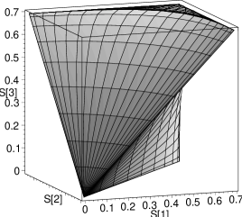
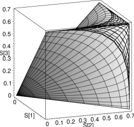
Figure 1: The Pod: Here is the space of all possible pure states of three spin-$\tfrac{1}{2}$ particles, shown from two angles. The “hiccup” or seam in the parametrisation lines is not a graphical artefact, it is the line where the pod surface ceases to be identical to the beechnut surface (see figure 3).

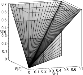
Figure 2: The Slice States: The von Neumann entropies for all three sets of slice states. The central spine linking all three fins is the subspace of generalised GHZ states, with the maximally entangled GHZ state at the top end, and the spin eigenstate at the bottom. The outside corners are the three possible two-particle maximally entangled states (with the other particle a bystander), and the edges running from those corners to the spin eigenstate have non-maximal two-particle entanglement, but are still bystander states. The edges that run from the points of each maximal two-particle entanglement to the maximal GHZ state are the slice ridges.

Figure 3: The Beechnut: Here’s how the Beechnut states got their name. These are the same graph, seen from two angles. Note that the dome at the top of the Beechnut doesn’t reach the maximally entangled GHZ state.

References

• [1] Schrödinger E., The Present Situation in Quantum Mechanics: A translation of Schrödinger’s “Cat Paradox” paper in Quantum Theory and Measurement eds Wheeler, J. A., and Zurek W. H., Princeton Series in Physics (1983) p152.
• [2] Lo, H. K., Popescu, S., and Spiller, T., Introduction to Quantum Computing and Information. World Scientific (1998), ISBN 981-02-3399-X
• [3] Popescu S., and Rohrlich D., Thermodynamics and the measure of entanglement. Phys. Rev. A. 56 R3319 (1997)
• [4] Vidal, G., Entanglement Monotones. J. Mod. Optics 47, 355 (2000); quant-ph/9807077
• [5] Thapliyal, A. V., On Multipartite Pure State Entanglement. Phys. Rev. A 59 3336 (1999); quant-ph/9811091
• [6] Bennett, C. H., Popescu S., Rohrlich D., Smolin J. A., and Thapliyal A. V., Exact and Asymptotic Measures of Multipartite Pure State Entanglement. quant-ph/9908073
• [7] Wootters, W. K., Quantum entanglement as a quantifiable resource. Phil. Trans. Roy. Soc. A 356, 1717 (1998)
• [8] Coffman, V., Kundu, J., and Wootters, W. K., Distributed Entanglement. Phys Rev A 61, 2306 (2000); quant-ph/9907047
• [9] Grassl, M., talk presented at the Isaac Newton workshop, Complexity, Computation and the Physics of Information Processing July 1999.
• [10] Horodecki, M., Horodecki, P., Horodecki, R., Limits for entanglement measures. Phys Rev Lett 84, 2014 (2000) quant-ph/9908065
• [11] Nielsen, M. A., Continuity bounds for entanglement. quant-ph/9908086
• [12] Vinberg E. B., and Onishchik, A. L., Seminar on Lie Groups & algebraic groups (Moscow, 1988) p. 144 (in Russian) English translation: Lie groups and algebraic groups (Springer series in Soviet Mathematics) Springer (1990) ISBN 3-540-50614-4, 0-387-50614-4, Chapter 3 “Algebraic Groups”, paragraph 4: “Compact Linear Groups”, Theorem 3: The orbits of a linear group acting in a real vector space are separated by the invariants.
• [13] Linden, N., and Popescu, S., On multiparticle entanglement. quant-ph/9711016 and Fortsch. Phys. 46, 567 (1998)
• [14] Schlienz, J., Ph.D. thesis.