Quantum limit of optical magnetometry in the presence of ac-Stark shifts
Abstract
We analyze systematic (classical) and fundamental (quantum) limitations of the sensitivity of optical magnetometers resulting from ac-Stark shifts. We show that in contrast to absorption-based techniques, the signal reduction associated with classical broadening can be compensated in magnetometers based on phase measurements using electromagnetically induced transparency (EIT). However due to ac-Stark associated quantum noise the signal-to-noise ratio of EIT-based magnetometers attains a maximum value at a certain laser intensity. This value is independent on the quantum statistics of the light and defines a standard quantum limit of sensitivity. We demonstrate that an EIT-based optical magnetometer in Faraday configuration is the best candidate to achieve the highest sensitivity of magnetic field detection and give a detailed analysis of such a device.
pacs:
42.50.Lc, 07.55.-w,07.60.-jI Introduction
The detection of magnetic fields by optical means is a well developed technique with applications ranging from geology and medicine [1] to fundamental tests of violations of parity and time-reversal symmetry [2].
In spite of their great variety, optical magnetometers can be divided in two basic classes. In the first class light absorption at a magnetic resonance is used to detect Zeeman level shifts, while the second class makes use of the associated changes of the index of refraction. So called optical pumping magnetometer (OPM) [1] as well as dark-state magnetometers based on absorption measurements [3] belong to the first class. The recently developed magnetometers based on phase-coherent atomic media [4, 5] and the mean-field laser magnetometer of ref.[6] belong to the second class.
If systematic measurement errors can be avoided, which in practice can be a challenging task, the smallest detectable Zeeman shift (in units of frequency) is determined by the ratio of the noise level of the signal to its rate of change with respect to frequency
| (1) |
A fundamental lower limit of results from photon counting errors due to shot-noise of the probe electromagnetic wave. , which characterizes a “quality factor” of the system, is determined by an effective width of the magnetic resonance. The ultimate goal of magnetometer design is to minimize the noise level and the effective width at the same time.
The width of magnetic resonances in optical magnetometers is subject to two types of broadening: resonant power-broadening due to the coupling of the optical fields to the probe-transition and a broadening due to ac-Stark shifts resulting from non-resonant couplings to other transitions. As shown in [4] and [5] power-broadening limits the simultaneous minimization of noise and in absorption based magnetometers. In such devices increasing the probe laser power reduces the shot-noise but does reduce the signal at the same time. As a consequence the sensitivity saturates at a rather low power level. On the other hand, as shown in [4] and [5], this effect can be compensated in a magnetometer that detects phase shifts of the probe electromagnetic wave propagating in an optically thick atomic medium under conditions of electromagnetically induced transparency (EIT) [7]. Theoretically a complete elimination is possible in a 3-level -type system.
In any real atomic system, however, there are non-resonant couplings to additional levels which lead to ac-Stark shifts and an additional broadening of the magnetic resonance proportional to the laser intensity. In the present paper we analyze the influence of ac-Stark shifts and show that they (i) can diminish the magnetometer signal and (ii) lead to additional noise contributions. We show that in absorption based devices ac-Stark broadening leads to a further reduction of the signal. In contrast it only gives rise to a bias phase shift in an phase-sensitive EIT magnetometer. This bias phase shift can be calibrated but is still a major source of systematic errors. It can be eliminated, if an EIT magnetometer with Faraday configuration is considered.
However, in both, absorptive and dispersive type devices, ac-Stark shifts give also rise to fundamental noise contributions which increase with the laser power more rapidly than shot noise. Hence the magnetometer sensitivity decreases above a certain power level. The maximum value of sensitivity constitutes the standard quantum limit. For an EIT magnetometer based on phase-shift measurements this limit is determined by the dispersion-absorption ratio of the medium and the intensity-phase noise coupling due to the self-phase modulation associated with ac-Stark shifts.
We also discuss the possibility of further increasing the sensitivity by means of non-classical light fields and show that the maximum sensitivity is essentially independent of the light statistics.
The paper is organized as follows: In Sec. II we discuss the fundamental broadening mechanisms of magnetic resonances, power-broadening and ac-Stark associated broadenings. It is shown in Sec. III that the classical signal reduction due to these broadenings can be compensated in phase-sensitive EIT magnetometers in contrast to absorption-based techniques. In Sec. IV fundamental quantum noise sources are discussed and the standard quantum limit of magnetometer sensitivity derived. A detailed analysis of an EIT-Faraday magnetometer is given in Sec. V and the prospects of using non-classical input states are discussed.
II broadening of magnetic resonances
Optical magnetometers measure in essence the position of certain resonances which are sensitive to magnetic level shifts. An important quantity that determines the signal strength of such a measurement is the width of the magnetic resonance. As a rule the narrower the resonance, the easier it is to detect level shifts.
Magnetic resonances with small natural width can be obtained e.g. by coupling Zeeman or hyperfine components of ground states in atoms either with an RF field or via an optical Raman transition. In an optical magnetometer these ground-state sub-levels are then coupled by laser fields to excited atomic states. The optical coupling is also used to detect energy shifts of the ground-state sub-levels induced by a magnetic field. However, at the same time this coupling leads to a broadening of the magnetic resonances via two mechanisms: (i) power-broadening and (ii) broadening due to ac-Stark shifts.
A Power-broadening
The first mechanism is power-broadening due to the resonant interaction with the probe transition. When the Rabi-frequency of the optical probe field exceeds the value
| (2) |
where is the unbroadened width of the magnetic resonance and the homogeneous linewidth of the optical transition, the magnetic resonance becomes power-broadened. (Here and below we assume that .) The effective width scales linearly with the Rabi-frequency of the optical field or the square root of the corresponding power
| (3) |
is some numerical pre-factor of order unity that depends on the specific model [5, 9]. This broadening effect leads to a substantial limitation of the signal in an optical pumping magnetometer, as shown in [5] and [9].
B Broadening due to ac-Stark shifts
The second broadening mechanism is due to non-resonant couplings of the probe electromagnetic wave with other than the probe transition and the associated ac-Stark shifts. The ac-Stark effect leads to a shift of the magnetic resonance of
| (4) |
where is some effective detuning of non-resonant transitions from the frequency of the probe field weighted with relative oscillator strengths. is again the Rabi-frequency of the probe field corresponding to the resonant probe transition. ( is of course just a model-dependent coupling parameter. We have used this notation here for simplicity of the discussions.)
In the classical limit and for a homogeneous laser intensity throughout the atomic vapor, there is only a constant frequency shift due to the ac-Stark effect. This shift can be calibrated. However, maximum signal is usually achieved when the atomic density is chosen such that there is a substantial absorption of the probe field. Hence when the probe Rabi-frequency exceeds the value
| (5) |
the resonance frequency changes as a function of propagation through the medium. This leads to an effective inhomogeneous broadening of the magnetic resonance. For example, the transmission of a cell containing atoms with a Lorentzian magnetic resonance subject to ac-Stark shifts is determined by the integrated imaginary part of the susceptibility ()
| (6) |
characterizes the -dependent power of the probe field and the detuning from the un-shifted transition frequency. It is easy to see, that there is a broadening of the magnetic resonance depending on the magnitude of the ac-Stark shifts and the details of the absorption process. An important feature is that this broadening is proportional to the square of the Rabi-frequency or the laser power. Thus above a certain power level, determined by Eq.(5) ac-Stark associated broadening can exceed power broadening, which leads e.g. to further reduction of the signal in an optical pumping magnetometer.
III compensation of broadening effects in EIT magnetometer
We here demonstrate that the classical broadening mechanisms discussed in the previous section do not necessarily lead to a reduction of the magnetometer signal if phase measurement techniques are used. It has been shown in detail in [5] and [8], that power-broadening can be completely compensated in a phase measurement by making use of EIT in optically dense -type systems.
The 3-level configuration of an EIT magnetometer as well as the associated linear susceptibility spectrum of the probe field are shown in Fig.1. Here and in the following we consider closed systems i.e. we assume that there are no effective decay mechanism due to time-of-flight limitations. The upper level of the probe-field transition is coupled to a meta-stable lower level by a coherent and strong driving field of Rabi-frequency . The probe field Rabi-frequency is denoted as () and the coherence decay rate of the probe transition as . is the one-photon detuning of the drive field and the two-photon detuning. The transverse decay rate of the two-photon resonance (magnetic resonance) is denoted as . It is assumed that the corresponding population exchange between the ground-state sub-levels is small and will be neglected
As in the case of an OPM there is power-broadening in an EIT magnetometer as soon as . A unique property of an EIT resonance is however that the dispersion-absorption ratio of the optical transition is given by the inverse of the width of the ground-state transition and is independent on the drive power if . Under conditions of one-photon resonance () one finds for small two-photon detuning
| (7) | |||||
| (8) |
The residual absorption at the EIT resonance decreases with increasing laser power in the same way as the dispersion. Thus in a phase shift measurement power broadening can be compensated by increasing the density and keeping a constant optical depth of the medium.
Similarly one finds that as long as the drive-field Rabi-frequency is large compared to probe-induced ac-Stark shifts, which is very well satisfied, ac-Stark shifts of the magnetic resonance (eq.(4)) lead only to a bias phase shift.
| (9) |
where is the length of the atomic vapor cell. This phase shift can in principle be calibrated but gives rise to systematic errors. As will be discussed in detail later on, there is no such bias phase shift in a resonant Faraday configuration.
We conclude this section by emphasizing that in phase-detection schemes based on EIT the detrimental (classical) effects of power-broadening and ac-Stark associated broadening are eliminated. In the following section we will discuss the fundamental quantum noise sources of such magnetometer schemes.
IV quantum-noise limit of magnetic field detection via optical phase shifts in the presence of ac-Stark effects
The problem of sensitive detection of phase shifts is common in optics. On the quantum level, the sensitivity of such kind of measurements is restricted by (i) vacuum fluctuations in the system and (ii) self-action noise due to nonlinearities in the system, as for example caused by ac-Stark shifts. The simultaneous presence of both noises usually leads to an absolute limit of the sensitivity.
Let us discuss this problem for the particular case of optical magnetometry based on phase-shift measurements in an atomic medium. The ultimate limit for the smallest detectable phase shift is set by the generalized uncertainty relation [10] between phase- [11] and photon-number fluctuations of the output field.
| (10) |
where denotes the anti-commutator. If phase- and photon-number fluctuations are uncorrelated, the second term on the r.h.s. vanishes and one recovers the familiar Heisenberg relation. In any real magnetometer schemes phase and intensity fluctuations are however correlated due to e.g. ac-Stark shifts (self phase modulation), and thus the second term in Eq.(10) is in general nonzero. When the intensity-phase coupling is small, it can be characterized by a linear coupling coefficient in the form , where denotes phase fluctuations not correlated to intensity fluctuations. Thus we find
| (11) |
The signal phase accumulated during the propagation through an atomic vapor cell is proportional to the Zeeman splitting , the length of the cell , and the dispersion of the real part of the susceptibility at the laser frequency . The cell length is restricted by the absorption at the laser frequency, and a reasonable upper limit for is the (amplitude) absorption length .
Thus the maximum phase shift is
| (12) |
One recognizes, that the sensitivity of phase measurements to Zeeman shifts is determined by the dispersion-absorption ratio .
The limit for the smallest detectable Zeeman shift is therefore given by
| (13) |
Under the condition, that the dispersion-absorption ratio is independent on the laser power, the r.h.s. of this expression is minimized when . Therefore there is an absolute lower limit or “quantum limit” of magnetic field detection via phase-shift measurements independent on the photon-number fluctuations
| (14) |
The absorption-dispersion ratio of a magnetic resonance is usually given by its natural width, which can be rather small if a two-photon Raman process between Zeeman- or hyperfine components is used as in an EIT magnetometer.
We will show later on that different measurement strategies as well as the use of non-classical light fields do in general not improve this result.
V EIT-based Faraday magnetometer
Let us now discuss in detail an EIT magnetometer in resonant nonlinear Faraday configuration. For this we consider the propagation of a strong, linear polarized light field through an optically dense medium, consisting of resonant -type systems (atoms, quantum wells etc.) as shown in Fig. 2. For simplicity we ignore optical pumping into lower states other than those shown in the figure and assume a closed system. For a resonant transition (say), optical pumping into the lower state depletes both states in the same way and thus effectively diminishes the optical density but does not affect the signal. Symmetric re-pumping can be used to maintain the population in the relevant sub-system without affecting the detection scheme. We include a dephasing of the ground-state coherence with rate and a population exchange rate between the ground states .
The two circular components and of the linear polarized light generate a coherent superposition (dark state) of the states . A magnetic field parallel to the propagation axis leads to an anti-symmetric level shift of and thus by virtue of the large linear dispersion at an EIT-resonance to an opposite change in the index of refraction for both components. As a result the polarization direction is rotated, which is the so-called resonant nonlinear Faraday effect [12]. The difference to the linear Faraday effect is the presence of the intensity-dependent dark resonance generated by the action of the strong laser field as opposed to a usual absorption resonance in the weak-field limit. The rotation of the plane of polarization at the output can be measured by detecting the intensity difference of two linear polarized components 45o rotated with respect to the input polarization.
An aspect of the system, which becomes particularly important when strong fields are considered, are non-resonant couplings of the two circular components to other levels, which to lowest order give rise to ac-Stark shifts of the states . In a Faraday configuration the ac-Stark shifts of and are exactly equal and opposite in sign due to symmetry and thus there is no average effect on the signal and no bias phase shift or rotation. Thus the Faraday magnetometer is not subject to systematic errors associated with ac-Stark shifts. However, as mentioned before, ac-Stark shifts cause a coupling between intensity and phase fluctuations which need to be taken into account.
A Detection scheme
We here consider the detection scheme shown in Fig. 3. A strong linear polarized field initially polarized in direction propagates through a cell of length with the magneto-optic medium. Due to the nonlinear Faraday effect the plane of polarization is rotated by an angle .
In order to detect this angle the intensity difference of the two orthogonal output directions and is measured. The operator for the number of counts is given by
| (15) |
where denote the positive and negative frequency part of the output electric field operators, is the measurement time, and , being the beam cross-section and the resonance frequency. Making use of the field commutation relations and , we can express the mean number of counts as well as the fluctuations in terms of normal-ordered correlation functions. The latter allows to apply a c-number approach where the operators are approximated by stochastic complex functions .
| (16) | |||||
| (17) |
where follows form Eq.(15) by replacing the field operators by c-numbers
| (18) |
In the usual configuration only the -polarized component of the input field is excited and we will restrict the discussion to a vacuum input of the -polarized component. The propagation of the field through the magneto-optical medium is most conveniently described in terms of right and left circular components , and we therefore have
| (19) |
The propagation of the circular components can be characterized by two parameters, the intensity transmission coefficient and the phase shift of the respective component at the output.
| (20) |
In the limit of small magnetic fields the absorption of both circular components is identical for symmetry reasons i.e. there is no dichroism. With this we obtain for cw-input fields
| (21) |
where is the (stationary) signal phase shift. Similarly we can estimate the fluctuations in lowest order of the small rotation angle in the case of an initially coherent field
| (22) |
The first term corresponds to the vacuum noise level and the second term proportional to
| (23) |
describes fluctuations due to an intensity-phase noise coupling in the medium. ()
In the following we calculate the loss factor , the signal phase shift and the fluctuations due to the intensity-phase noise coupling for the EIT-Faraday magnetometer.
B Medium susceptibility and field propagation
The stationary propagation of the right and left circular polarized electric field components through the atomic vapor is described by Maxwell equations in slowly-varying amplitude and phase approximation
| (24) |
is the atomic number density, are the dipole moments of the respective transitions, and are the c-number analogues of the atomic lowering operators . Analytic expressions for can be obtained from the stationary solution of the c-number Bloch equations for the atomic populations
| (26) | |||||
| (28) | |||||
and polarizations
| (30) | |||||
| (31) |
where
| (32) | |||||
| (33) |
is the radiative linewidth of the transitions , and is the homogeneous transverse linewidth of the optical transitions . is the Zeeman splitting and are the ac-Stark shifts of levels . are the complex Rabi-frequencies of the two optical fields, . We have disregarded Langevin noise forces in Eqs.(26-31) associated with spontaneous emission and collisional decay processes, since it was shown in [5] that atomic noises have a negligible effect on the magnetometer sensitivity.
We calculate the stationary solutions of the Bloch-equations by considering only the lowest order in , , and . In this limit we find
| (36) | |||||
where . Usually the coherence decay between the ground levels dominates the population exchange and thus .
It is convenient to separately consider the spatial evolution of amplitudes and phases of the complex Rabi-frequencies . The intensities of the two fields are attenuated in the same way
| (37) |
where .
Eq. (37) can be easily solved when the length of the cell is small enough, such that . In the Faraday set-up discussed here , and therefore . We thus arrive at
| (38) | |||||
| (39) |
It is interesting to note that under conditions of EIT the residual absorption is not exponential but linear. The intensity transmission coefficient is then given by
| (40) |
The approximation sets an upper limit for the losses, such that .
Similarly we find the phase equations
| (41) | |||||
| (42) |
The contributions from the one-photon detuning cancel when the relative phase is considered
| (43) |
The first term describes the signal-phase shift due to a magnetic field and the second term the ac-Stark contribution. Integration of Eq.(43) yields for the signal
| (44) |
and the ac-Stark contribution
| (45) |
C Ac-Stark shifts and associated noise
Let us now discuss the average ac-Stark shift and the corresponding noise contributions. For this we first consider the effect of an off-resonant quantized field on the energy of a single atom in lowest non vanishing order of perturbation. We then generalize the results for the average ac-Stark shift and its fluctuations to an ensemble of atoms by making the physically reasonable assumption that ac-Stark shifts of different atoms are uncorrelated.
We decompose the Hamiltonian of the single atom interacting with the quantized field in a rotating frame in the form , where is the unperturbed part
| (47) | |||||
and are the detunings of the and transitions.
| (48) | |||
| (49) |
describes the resonant and non-resonant couplings of the quantized fields to the atom. The non-resonant couplings to the excited states cause ac-Stark shifts. We here have assumed that both fields are nearly monochromatic and have set the energy of level equal to zero. are the dipole moments of the transitions .
We proceed by formally eliminating the excited states by means of a canonical transformation in second order perturbation
| (50) |
where obeys the equation
| (51) |
Under conditions of exact two-photon resonance for the fields we obtain the transformation operator
| (52) |
Assuming that the population of all excited levels is small, we eventually find for the transformed Hamiltonian
| (53) | |||
| (54) | |||
| (55) |
Let us assume now, that is much larger than the natural width of the excited states, and therefore the population transfer due to the non-resonant coupling is negligible. We identify , where is some effective detuning. The dipole moments and have usually alternating signs for different excited states . We therefore set . Then the ac-Stark shift of the single atom can be represented by the operator expression
| (56) |
where specifies the atom and its location. Thus we find for the average ac-Stark shift
| (57) |
where . Similarly we obtain for the second-order moments of the ac-Stark shifts
| (58) | |||
| (59) | |||
| (60) | |||
| (61) |
or after normal ordering
| (62) | |||
| (63) | |||
| (64) | |||
| (65) | |||
| (66) |
The first terms in Eqs.(64) and (66) correspond to classical fluctuations, while the second term in (64) is vacuum or shot noise. If the applied fields are in a coherent state only the shot noise term survives. In any practical realizations there are however large excess noise contributions and the first terms are usually the dominant ones. We will show that all excess noise contributions are canceled in a Faraday magnetometer and only the vacuum contribution survives.
We generalize the above single-atom results to an ensemble of atoms assuming independent fluctuations of the ac-Stark shifts of different atoms, i.e.
| (67) |
where . We introduce the continuous variable
| (68) |
In a continuum approximation, , and we have
| (69) |
Similarly
| (70) | |||
| (71) | |||
| (72) |
and
| (73) | |||
| (74) |
We here have used that in continuum approximation for any smooth function holds
| (75) |
It is now straight forward to evaluate the quadratic deviation of the relative ac-Stark shift
| (76) | |||
| (77) |
We note that the classical excess noise contributions exactly cancel and only the vacuum contribution is left over. Due to the intrinsic balancing in the EIT-Faraday magnetometer excess noise contributions are automatically canceled. This is an important advantage of the Faraday configuration as compared to the asymmetric EIT-magnetometer discussed in [4] and [5].
D Signal-to-noise ratio and minimum detectable Zeeman shift
The minimum detectable Zeeman shift is obtained by setting the mean number of counts
| (79) |
equal to the quantum mechanical uncertainty
| (80) | |||
| (81) |
This yields the signal-to-noise ratio
| (82) |
which is maximized for an optimal power of the field corresponding to
| (83) |
Substituting the optimum Rabi-frequency (83) into (82) yields a maximum SNR for . Thus we find the quantum limit for the detection of Zeeman level shifts
| (84) |
where
| (85) |
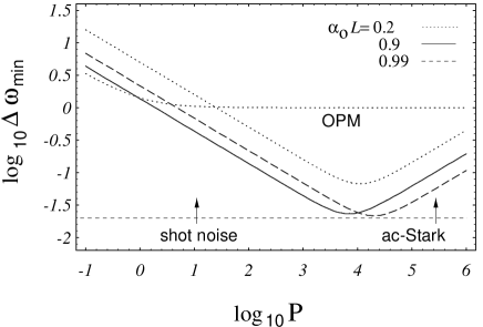
is a numerical factor which varies between 1 and 2 for . (Note that is the transmission coefficient under conditions of EIT. Without EIT the medium would be totally opaque.) In Fig. 4 we have shown the minimum detectable Zeeman splitting (proportional to the magnetic field) as function of the laser input power for different transmission coefficients.
One clearly sees that for small laser powers shot-noise is dominant, while for larger laser powers ac-Stark associated fluctuations take over. Also shown is the saturation behavior of an OPM [5]. Due to power broadening the sensitivity of an OPM saturates as soon as the Rabi-frequency reaches the value . In the EIT-Faraday magnetometer, on the other hand, the optimum Rabi-frequency corresponding to the quantum limit is of the order of . Since much higher sensitivities can be achieved here.
E Compensation of ac-Stark associated noise by use of non-classical input fields
It is well known, that the effect of self-phase modulation due to refractive nonlinearities can be compensated, at least in part, by means of an optimum detection procedure (for example, by measuring not the phase, but an appropriately chosen quadrature amplitude of the probe electromagnetic wave) and/or by using non-classical light [13, 14]. The properties of the input quantum state in the methods utilizing non-classical light are thereby chosen such that after the interaction the probe wave is in the coherent or phase-squeezed state.
In the case of an optical magnetometer, ac-Stark shifts appear due to non-resonant nonlinearities and it would seem that these shifts can in principle be compensated by an adapted measurement strategy and the use of non-classical light. An essential condition for such methods is however that the system is nearly lossless in order to preserve the non-classical state of light. On the other hand, as discussed above, the maximum signal in an optical magnetometer is achieved under conditions of substantial absorption. (We note that the SNR is proportional to ln.) We will show in the following with simple estimates that this feature makes it impossible to increase the sensitivity by using non-classical light.
Let us consider the simplest example of compensation of ac-Stark associated noise by non-classical light. We assume, that the slowly varying field operators in the Heisenberg picture are represented in the form , where is the fluctuation part. To discuss the compensation of ac-Stark effects let us disregard the resonant coupling with the medium and the associated absorption. Then we find that the field fluctuations at the end of the vapor cell can be written as
| (86) | |||
| (87) |
The second terms in these equations are due to ac-Stark shifts. One can see that the uncertainty of the phase difference increases as a result of ac-Stark shifts, which leads to the sensitivity restriction, discussed above.
Let us assume now, that the incident field is squeezed in such a way, that the operators of the field fluctuations at the input obey the relations
| (88) | |||
| (89) |
Here are free-field operators (the corresponding state is the field vacuum), which obey the commutation relations and . Then, in the absence of losses, the effects of ac-Stark shifts are completely compensated in the output and the output fields are coherent.
| (90) | |||
| (91) |
The sensitivity of the phase measurement would thus be determined by shot-noise only, .
In the absence of losses, the sensitivity of the detection can even be better than the shot-noise limit, if the initial state of the field is appropriately chosen [14]. Making use of a SU(2) Lie-group description, Yurke showed that the sensitivity of a phase shift measurement in a Mach-Zehnder interferometer can approach the so-called Heisenberg limit , where is the total number of registered quanta [15, 16].
However, in the presence of losses resulting from the resonant coupling the noise compensation by means of non-classical light is only partial due to unwanted noises added by the medium. Taking into account linear losses and assuming, that the entrance field is squeezed in the way discussed above, we can rewrite the equation for the residual noises in the phase as follows:
| (92) |
is the -dependent transmission coefficient. The expression indicates, that for small losses in the medium, the noise can be almost completely suppressed. A maximum signal is achieved however when and thus the use of non-classical light only leads to a marginal reduction of the ac-Stark associated noise. This is in contrast to the measurement schemes discussed in [13, 14] which utilize squeezing to improve sensitivity. The change of the expression for the ac-Stark associated noise leads to a change of the sensitivity factor according to
| (93) |
It is easy to see, that for all relevant values of , which means that squeezing does not improve the sensitivity of the detection.
The same conclusion can be drawn for any kind of optimal strategy of measurement to compensate ac Stark shifts. The main reason for this is that both, the magnitude of the signal and absorption losses increase with the density-length product of the atomic vapor cell.
VI Summary
We have discussed the influence of ac-Stark shifts on the sensitivity of optical magnetometers. We have shown that these shifts cause a broadening of the relevant resonances and give rise to additional noise contributions. In absorption-type magnetometers, such as OPMs, the ac-Stark associated broadening as well as power-broadening lead to a reduction of the signal. We have shown that the classical part of these effects can be completely compensated in an EIT magnetometer in Faraday configuration where polarization rotation or, equivalently, the relative phase shift of two circular components is measured.
In a magnetometer based on phase measurements ac-Stark shifts lead also to a coupling between intensity and phase fluctuations. As a result there are additional, ac-Stark associated fluctuations which dominate over shot noise beyond a critical laser power. For a certain optimum intensity the fundamental signal-to-noise ratio attains a maximum value which represents the standard quantum limit of optical magnetometer based on phase-shift measurements. This quantum limit is determined by the dispersion-absorption ratio of the atomic medium and the strength of the intensity-phase noise coupling. The unique property of EIT is to provide a dispersion-absorption ratio which is independent of power-broadening and is given by the lifetime of a ground-state coherence. The minimum magnetic level shift corresponding to the quantum limit of EIT magnetometers can thus be orders of magnitude smaller than that of optical pumping devices.
We have shown that the best candidate to reach the standard quantum limit is a magnetometer in Faraday configuration, which has been analyzed in detail. In an EIT-Faraday magnetometer the signal reduction due to power- and ac-Stark broadenings is compensated by large densities of the atomic vapor. The influence of classical excess noise is completely eliminated due to symmetry and there are much less sources for systematic errors. We have also shown that the use of non-classical light and different detection techniques only marginally improves the attainable sensitivity since a maximum signal is associated with substantial losses in the atomic medium.
Acknowledgements
The authors would like to thank M. Lukin for stimulating discussions on the role of ac-Stark shifts. A.M. and M.O.S. gratefully acknowledge further useful discussions with Y. Rostovtsev and the support from the Office of Naval Research, the National Science Foundation, the Welch Foundation, the Texas Advanced Research and Technology Program and the Air Force Research Laboratories. M.F. gratefully acknowledges the financial support of the Alexander-von-Humboldt foundation through the Feodor-Lynen Program.
REFERENCES
- [1] for a review on optical pumping magnetometers see: E. B. Alexandrov and V. A. Bonch-Bruevich, Opt. Eng. 31, 711 (1992); E. B. Alexandrov et al., Laser Physics 6, 244 (1996).
- [2] E. A. Hinds, Atomic Physics Vol.11 (1988), S. Haroche, J. C. Gray and G. Gryndberg, Eds.; L. R. Hunter, Science 252, 73 (1991); D. Budker, V. Yashchuk, and M. Zolatorev, Phys. Rev. Lett.81, 5788 (1998); V. Yashuk et al. preprint LBNL-42228 (1998).
- [3] A. Nagel et al., Europhys. Lett. 44, 31 (1998).
- [4] M. O. Scully and M. Fleischhauer, Phys. Rev. Lett. 69, 1360 (1992).
- [5] M. Fleischhauer and M. O. Scully, Phys. Rev. A 49, 1973 (1994).
- [6] F. Bretenaker, B. Lépine, J. C. Cotteverte, and A. Le Floch, Phys. Rev. Lett. 69, 909 (1992).
- [7] for a review on EIT see: S. E. Harris, Physics Today 50, 7, 36 (1997).
- [8] M. D. Lukin, M. Fleischhauer, A. S. Zibrov, H. G. Robinson, V. L. Velichansky, L. Hollberg, and M. O. Scully, Phys. Rev. Lett. 79, 2959 (1997).
- [9] M. Fleischhauer and M. O. Scully, Quantum Semiclass. Opt. 7, 297 (1995).
- [10] H. P. Robertson, Phys. Rev. A 35, 667 (1930); E. Schrödinger, “Zum Heisenbergschen Unschärfeprinzip”, Ber. Kgl. Akad. Wiss., Berlin, p.296, 1930;
- [11] Although there is no rigorous definition of a hermitian phase operator, we nevertheless use it here noting that we restrict ourselves to states of the radiation field which have no significant overlap with the vacuum. In this case phase and photon number operators nearly coincide with the phase and amplitude quadrature operators.
- [12] W. Gawlik, J. Kowalski, R.Neumann, and F. Träger, Phys. Lett. A48, 283 (1974); W. Gawlik, in Modern Nonlinear Optics, part 3, M. Evans and S. Kielich, eds., Wiley (1994); K. H. Drake, W. Lange, and J. Mlynek, Opt. Comm. 66, 315 (1988); S. Giraud-Cotton et al. Phys.Rev.A 32, 2211 (1985), ibid 2223 (1985); L. M. Barkov et al. Opt.Comm. 70, 467 (1989); F. Schuller et al. ibid 71, 61 (1989).
- [13] C. M. Caves, Phys. Rev. D 23, 1693 (1981).
- [14] W. G. Unruh, in Quantum Optics, Experimental Gravitation, and Measurement Theory, eds. P. Meystre and M. O. Scully, (Plenum, 1982), p. 647; M. T. Jaekel and S. Reynaud, Europhys. Lett. 13, 301 (1990); D. V. Kupriyanov and I. M. Sokolov, Quantum Opt. 4, 55 (1992); A. F. Pace, M. J. Collett and D. F. Walls, Phys. Rev. A 47, 3173 (1993); S. P. Vyatchanin and A. B. Matsko, JETP 77, 218 (1993); G. J. Milburn, K. Jacobs, and D. F. Walls, Phys. Rev. A 50, 5256 (1994).
- [15] B. Yurke, S. L. McCall, J. R. Clauder, Phys. Rev. A 33, 4033 (1986).
- [16] C. Brif and A. Mann, Phys. Rev. A 54, 4505 (1996); T. Kim, O. Phister, M. J. Holland, J. Noh, and J. L. Hall, Phys. Rev. A 57, 4004 (1998) and references therein.