Hardy-type experiment for the maximally entangled state: Illustrating the problem of subensemble postselection

Abstract

By selecting a certain subensemble of joint detection events in a two-particle interferometer arrangement, a formal nonlocality contradiction of the Hardy type is derived for an ensemble of particle pairs configured in the maximally entangled state. It is argued, however, that the class of experiments exhibiting this kind of contradiction does not rule out the assumption of local realism.

PACS: 03.65.Bz

Key words:  Two-particle interferometry; Subensemble postselection; Hardy’s
nonlocality theorem; Bell’s inequality; Interaction-free measurement

1 Introduction

A remarkable feature of Hardy’s nonlocality theorem [1, 2] is that it applies to any pure entangled states of a bipartite two-level system, except, curiously, those states which are maximally entangled such as the singlet state of two spin-half particles. As Hardy says [1], “The reason for this is that the proof relies on a certain lack of symmetry that is not available in the case of a maximally entangled state.” Indeed, for this class of states, every single-particle observable is perfectly, symmetrically correlated with some other observable associated with the other particle. As a result, the set of Hardy equations (3a)-(3d) (see below) upon which the nonlocality contradiction is constructed cannot be satisfied for the maximally entangled case [3, 4]. An attempt to extend Hardy’s theorem to cover maximally entangled state was made by Wu et al. in Ref. [5] where the authors, using a quantum-optical setting, demonstrate local-realism violations for a maximally entangled state of two particles without using inequalities. It was later pointed out [6], however, that the nonlocality argument in [5] requires a minimum total of six dimensions in Hilbert space, and so there is no contradiction with the fact that no Hardy-type nonlocality argument can be constructed for the maximally entangled state if the observables to be measured on each particle are truly dichotomic. The extra dimensions needed to properly describe the experiment in Ref. [5] arise due to the use of three independent detectors for each of the particles. Moreover, the probabilistic nonlocality contradiction derived in [5] is conditioned on the fact that the statistical analysis involved is restricted to a particular subensemble of joint detection events. The authors define this subensemble by saying that [5], “We shall only be interested in those runs of the experiment for $K=L=0$, which means that particle 1 does not go to end $k$, while at the same time particle 2 does not go to end $l$.” Although there are situations in which subensemble selection may be a legitimate means to observe local-realism violations [7, 8, 9], we will see that this is not the case for the class of experiments considered in this Letter. Specifically, by using an arrangement for two-particle interferometry, we will show that, (a) if each particle is subjected to a single ideal (von Neumann-type) measurement (chosen at random between two such possible measurements), then it is necessary to perform subensemble postselection (or, equivalently, to reject some ‘undesirable’ subset of measurement data) if we want to obtain a Hardy-type nonlocality contradiction for the maximally entangled state; and (b) this procedure to get local-realism violations does not constitute a valid method to rule out all possible local hidden variable models since, for the class of experiments discussed, no Bell-type inequality is violated if the whole ensemble of measurement data is included in the statistical analysis. The conclusion to be drawn from these two statements is that the class of experiments adhering to Wu et al.’s approach does not provide a true test of quantum mechanics versus local realism, not even in the case of ideal behaviour of the experimental hardware.

The Letter is organized as follows. In Section 2 we consider a two-particle interferometer arrangement where a source emits pairs of particles, 1 and 2, in some quantum-mechanical superposition state. The outgoing particle 1 (2) is monitored by ideal detectors $L_{1}$ and $U_{1}$ ($L_{2}$ and $U_{2}$) so that, for this arrangement, each particle is subjected to a binary choice between the detection in either $L_{i}$ or $U_{i}$ (where $i=1$ (2) for particle 1 (2)). We will show that, under this dichotomic choice, no Hardy-type contradiction can be obtained when the experiment is performed on an ensemble of particle pairs prepared in the maximally entangled state (1) (see below). In Section 3, the ‘standard’ interferometric arrangement used in Section 2 is modified so that a partially absorbing material is placed in one of the routes available to one of the particles (say, particle 2) inside the interferometer. Naturally, the absorber is a kind of detector (call it, say, $A_{2}$) which detects some of the particles, namely those which are absorbed, while the rest pass through. Therefore, particle 2 is no longer subjected to a binary choice since it can be detected in either $L_{2}$, $U_{2}$, or $A_{2}$. The measurement data we are interested in will now consist of the subensemble of registration events for which both particles in a pair end at the corresponding detector $L_{i}$ or $U_{i}$, while the remaining two-particle coincidence detections (namely, those for which particle 1 ends in either $L_{1}$ or $U_{1}$ while particle 2 gets absorbed before reaching $L_{2}$ or $U_{2}$) are discarded. On the other hand, as shown in Refs. [10, 11], Hardy’s nonlocality argument can be cast in the form of an inequality which is just a particular case of the Clauser-Horne (CH) inequality [12, 13]. As we shall see, this inequality is violated for the above selected subensemble of joint detection events. The amount of this violation is found to be as large as $\frac{1}{2}\leq 0$. However, since this approach does involve a postselection procedure, then, it can be justifiably claimed [14] that one runs directly into the so-called subensemble postselection problem [12, 13, 14, 15, 16, 17] which, in our case, essentially means that the above local-realism violation would not be truly significant, as a Bell inequality could always be violated (even by purely classical correlations [17]) if one restricts the analysis to a suitable subensemble of the original ensemble of particle pairs. In Section 4 it is shown that, in fact, no CH inequality is violated if the entire pattern of localization correlations is analysed. Finally, in Section 5, we show how our interferometer set-up can be used to perform an interaction-free measurement of the presence of the absorber. Conclusions are presented in Section 6.

2 Failure of Hardy’s proof for the maximally entangled state in the standard interferometer set-up

In what follows we specialize in photons, although any other suitable interfering particle could equally be considered. For the present purpose, we consider a two-photon interferometer arrangement of the kind first discussed by Horne and Zeilinger [18] (see Fig. 1).

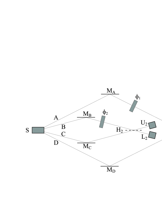
Fig. 1: An arrangement for two-particle interferometry of the kind proposed in Ref. [18]. All four detectors $L_{i}$ and $U_{i}$ ($i=1,2$) are assumed to be 100% efficient. Eventually, we will consider a modified version of this arrangement in which photon 2 has a nonvanishing probability of being absorbed by the phase shifter placed in path $B$.

A parametric down-conversion source is arranged to emit an ensemble of photon pairs along the beams $A$, $B$, $C$, and $D$, in such a way that the two photons 1 and 2 in each pair emerge coherently downstream from the source in the state

$$\left|\psi\right\rangle\,=\,\frac{1}{\sqrt{2}}\left(\left|A\right\rangle_{1}\left|C\right\rangle_{2}+\left|D\right\rangle_{1}\left|B\right\rangle_{2}\right),$$ (1)

where ket ${|A\rangle}_{1}$ designates photon 1 in beam $A$, etc. Beams $A$ and $D$ ($B$ and $C$) are totally reflected by respective mirrors $M_{A}$ and $M_{D}$ ($M_{B}$ and $M_{C}$), and subsequently recombined at the (nonpolarising) beam splitter $H_{1}$ ($H_{2}$) from which photon 1 (2) proceeds either to detector $L_{1}$ or $U_{1}$ ($L_{2}$ or $U_{2}$). Figure 1 also shows two adjustable phase shifters $\phi_{1}$ and $\phi_{2}$ placed into beams $A$ and $B$, respectively. For the initial state (1), and for symmetric, 50-50 beam splitters and lossless optical elements, the probabilities of joint detection of the two photons by the various detectors are, in an obvious notation,

$$P(L_{1},\phi_{1};L_{2},\phi_{2}) =P(U_{1},\phi_{1};U_{2},\phi_{2})=\tfrac{1}{4}\left[1+\cos(\phi_{1}-\phi_{2})\right],$$ (2a)

$$P(L_{1},\phi_{1};U_{2},\phi_{2}) =P(U_{1},\phi_{1};L_{2},\phi_{2})=\tfrac{1}{4}\left[1-\cos(\phi_{1}-\phi_{2})\right].$$ (2b)

It is easy to show that, in these cirscumstances, no Hardy-type contradiction can be obtained for the maximally entangled state (1). For the interferometric arrangement we are considering, Hardy’s argument for nonlocality involves four alternative experimental configurations each of which being characterized by a particular setting of the phase shifters. Specifically, these four configurations are defined by the respective settings: $(\phi_{1},\phi_{2})$, $(\phi_{1},\phi^{\prime}_{2})$, $(\phi^{\prime}_{1},\phi_{2})$, and $(\phi^{\prime}_{1},\phi^{\prime}_{2})$, where the first (second) entry inside each bracket is the value of the phase shifter acting on beam $A$ ($B$). In terms of joint detection probabilities, the state of the emerging down-converted pair of correlated photons will show Hardy-type nonlocality contradiction if the following four conditions are simultaneously fulfilled for such a state

$$P(L_{1},\phi_{1};L_{2},\phi_{2}) =0\,,$$ (3a)

$$P(U_{1},\phi_{1};U_{2},\phi_{2}^{\prime}) =0\,,$$ (3b)

$$P(U_{1},\phi_{1}^{\prime};U_{2},\phi_{2}) =0\,,$$ (3c)

$$P(U_{1},\phi_{1}^{\prime};U_{2},\phi_{2}^{\prime}) >0\,.$$ (3d)

Using predictions (3a)-(3d) one can construct an argument against the notion of local realism. In short, the argument is like this [1]: Suppose that, for a particular run of the experiment, we get photon 1 at $U_{1}$ and photon 2 at $U_{2}$ when the interferometer set-up is operated in the configuration $(\phi^{\prime}_{1},\phi^{\prime}_{2})$. From Eq. (3d), there is a nonzero probability for this joint detection event to occur. (We further assume that the event corresponding to detection of photon 1 in $L_{1}$ or $U_{1}$ is spacelike separated from that corresponding to detection of photon 2 in $L_{2}$ or $U_{2}$.) Then, by invoking local realism, and taking into account the prediction (3c), we can deduce that, had the phase shifter in path $B$ been set to $\phi_{2}$, photon 2 would have been detected in $L_{2}$. Likewise, from prediction (3b), and according to local realism, we can assert that photon 1 would have ended in $L_{1}$, had the phase shifter in path $A$ been set to $\phi_{1}$. Therefore, by combining the assumption of local realism with the quantum predictions (3d), (3c), and (3b), we are led to conclude that there is a nonzero probability that both photons in a pair end in the corresponding $L$-detector when the configuration is set to $(\phi_{1},\phi_{2})$. The remaining quantum prediction in Eq. (3a), however, tells us that no joint detection of photons 1 and 2 in $L_{1}$ and $L_{2}$ will take place when the interferometer set-up is arranged to operate in the configuration $(\phi_{1},\phi_{2})$. Hence a contradiction between quantum mechanics and local realism arises without using inequalities.

Now, if conditions (3a), (3b), and (3c) are to be fulfilled for the state (1), and assuming that the joint detection probabilities accounting for our experiment are those given by Eqs. (2a) and (2b), it is necessary that (see Eq. (2a)) $\phi_{1}-\phi_{2}=n_{1}\pi$, $\phi_{1}-\phi^{\prime}_{2}=n_{2}\pi$, and $\phi^{\prime}_{1}-\phi_{2}=n_{3}\pi$, with $n_{1},n_{2},n_{3}=\pm 1,\pm 3,\ldots$ . From these three equalities we obtain immediately that $\phi^{\prime}_{1}-\phi^{\prime}_{2}=\linebreak(n_{2}+n_{3}-n_{1})\pi$. As the number $n_{2}+n_{3}-n_{1}$ is an odd integer, we have $\cos(\phi^{\prime}_{1}-\phi^{\prime}_{2})=-1$, and then $P(U_{1},\phi_{1}^{\prime};U_{2},\phi_{2}^{\prime})=0$. So, the fulfillment of all three conditions (3a), (3b), and (3c), precludes the fulfillment of the condition in Eq. (3d), and thus no Hardy-type contradiction will be obtained for the maximally entangled state if each particle is subjected to a binary choice between detection in either $L_{i}$ or $U_{i}$. This impossibility can equivalently be established by stating that the fulfillment of conditions (3a)-(3c) by the state (1) implies that $P(L_{1},L_{2})=P(U_{1},U_{2})=0$ and $P(L_{1},U_{2})=P(U_{1},L_{2})=1/2$ for any one of the four configurations $(\phi_{1},\phi_{2})$, $(\phi_{1},\phi^{\prime}_{2})$, $(\phi^{\prime}_{1},\phi_{2})$, and $(\phi^{\prime}_{1},\phi^{\prime}_{2})$. Clearly this means that, for such configurations, whenever photon 1 is detected at $L_{1}$ ($U_{1}$) then with certainty photon 2 will be detected at $U_{2}$ ($L_{2}$), and vice versa. So, if one assigns a value ‘$-1$’ (‘$+1$’) to a count in either $L_{1}$ or $L_{2}$ ($U_{1}$ or $U_{2}$), then the expectation value of the product of the two outcomes over a large number of counts will be $E(\phi_{1},\phi_{2})=E(\phi_{1},\phi^{\prime}_{2})=E(\phi^{\prime}_{1},\phi_{2})=E(\phi^{\prime}_{1},\phi^{\prime}_{2})=-1$. These four perfect correlations, however, saturate the Bell-CHSH inequality [13, 19, 20]

$$\left|E(\phi_{1},\phi_{2})+E(\phi_{1},\phi^{\prime}_{2})+E(\phi^{\prime}_{1},\phi_{2})-E(\phi^{\prime}_{1},\phi^{\prime}_{2})\right|\leq 2.$$ (4)

So it is concluded, once again, that, for the interferometric arrangement under consideration, the maximally entangled state (1) cannot be used to exhibit Hardy-type nonlocality.

3 Hardy-like proof for the maximally entangled state in the modified interferometer set-up

Now the question arises about how to modify the ‘standard’ interferometer set-up we have used, in order that the resulting joint detection probabilities for the initial state (1) do satisfy all four conditions (3a)-(3d). The basic step towards this end is to introduce a partially absorbing material into one of the paths available to either one of the photons (say, photon 2), so that, actually, only a certain subensemble of the whole ensemble of emitted photon pairs is analysed for coincidences (see below). This subensemble will consist of all those pairs of photons 1 and 2 for which photon 2 is not absorbed and so ends up either in detector $L_{2}$ or $U_{2}$ (photon 1 always ends either in $L_{1}$ or $U_{1}$). In the following we shall assume that the phase shifter in beam $B$, besides imparting a variable phase shift $\phi_{2}$ to it, multiplies the amplitude of that beam by $u$ (with $0\leq u\leq 1$). More precisely, $u$ is the probability amplitude that a photon striking into this phase shifter passes straight through it, while $v$ is the probability amplitude that the photon gets absorbed (or, more generally, scattered), hence $u^{2}+v^{2}=1$. Therefore, the state of a photon propagating along path $B$ will evolve upon interacting with the phase shifter as

$$\left|B\right\rangle_{2}\rightarrow i\left(ue^{i\phi_{2}}\left|L_{2}\right\rangle+v\left|PS^{\ast}\right\rangle\right),$$ (5)

where the factor $i$ arises from reflection at $M_{B}$, $\left|L_{2}\right\rangle$ denotes the photon transmitted towards detector $L_{2}$, and $\left|PS^{\ast}\right\rangle$ denotes an excited state of the phase shifter due to the absortion of the photon (of course, the amplitude of absortion $v$ is generally complex, although this is not relevant for our purpose).

Another necessary modification with respect to the standard experimental set-up is that the beam splitter $H_{i}$, $i=1,2$, is no longer assumed to be 50-50 (for simplicity, we suppose that it continues to be symmetric), so that its reflectivity $r_{i}$ and transmittivity $t_{i}$ are any positive real numbers satisfying the relation $r_{i}^{2}+t_{i}^{2}=1$. So, any given experimental configuration for our interferometer set-up is now defined by the values of the local parameters $\phi_{1}$, $r_{1}$ (or $t_{1}$), $\phi_{2}$, $r_{2}$ (or $t_{2}$), and $u$. In particular, the four configurations involved in Hardy’s nonlocality argument are determined by the respective settings: $(\Phi_{1},\Phi_{2})$, $(\Phi_{1},\Phi^{\prime}_{2})$, $(\Phi^{\prime}_{1},\Phi_{2})$, and $(\Phi^{\prime}_{1},\Phi^{\prime}_{2})$, where the arguments $\Phi_{1}$, $\Phi^{\prime}_{1}$, $\Phi_{2}$, and $\Phi^{\prime}_{2}$ are a shorthand for the parameters ($\phi_{1},\,r_{1}$), ($\phi^{\prime}_{1},\,r^{\prime}_{1}$), ($\phi_{2},\,r_{2},\,u$), and ($\phi^{\prime}_{2},\,r^{\prime}_{2},\,u^{\prime}$), respectively. With all these ingredients, and taking into account the transformation (5), we can calculate again the joint probabilities in Eq. (2a) for the initial state (1). These are given by

$$P(L_{1},\Phi_{1};L_{2},\Phi_{2}) =\tfrac{1}{2}\left[u^{2}r_{1}^{2}t_{2}^{2}+t_{1}^{2}r_{2}^{2}+2ur_{1}r_{2}t_{1}t_{2}\cos(\phi_{1}-\phi_{2})\right],$$ (6a)

$$P(U_{1},\Phi_{1};U_{2},\Phi_{2}) =\tfrac{1}{2}\left[u^{2}t_{1}^{2}r_{2}^{2}+r_{1}^{2}t_{2}^{2}+2ur_{1}r_{2}t_{1}t_{2}\cos(\phi_{1}-\phi_{2})\right].$$ (6b)

Of course, in the case in which $r_{i}=t_{i}=1/{\sqrt{2}}$, and $u=1$, we retrieve the probabilities in Eq. (2a). Hardy’s nonlocality conditions are now defined by

$$P(L_{1},\Phi_{1};L_{2},\Phi_{2}) =0\,,$$ (7a)

$$P(U_{1},\Phi_{1};U_{2},\Phi_{2}^{\prime}) =0\,,$$ (7b)

$$P(U_{1},\Phi_{1}^{\prime};U_{2},\Phi_{2}) =0\,,$$ (7c)

$$P(U_{1},\Phi_{1}^{\prime};U_{2},\Phi_{2}^{\prime}) >0\,.$$ (7d)

So, in view of Eqs. (6a) and (6b), we must have the following relations in order for the conditions (7a), (7b), and (7c), respectively, to be satisfied by the state (1)

$$\cos(\phi_{1}-\phi_{2}) =-\frac{u^{2}r_{1}^{2}t_{2}^{2}+t_{1}^{2}r_{2}^{2}}{2ur_{1}r_{2}t_{1}t_{2}},$$ (8a)

$$\cos(\phi_{1}-\phi_{2}^{\prime}) =-\frac{(u^{\prime})^{2}t_{1}^{2}(r_{2}^{\prime})^{2}+r_{1}^{2}(t_{2}^{\prime})^{2}}{2u^{\prime}r_{1}r_{2}^{\prime}t_{1}t_{2}^{\prime}},$$ (8b)

$$\cos(\phi_{1}^{\prime}-\phi_{2}) =-\frac{u^{2}(t_{1}^{\prime})^{2}r_{2}^{2}+(r_{1}^{\prime})^{2}t_{2}^{2}}{2ur_{1}^{\prime}r_{2}t_{1}^{\prime}t_{2}}.$$ (8c)

It is straightforward to see that the right-hand side for each of the Eqs. (8a)-(8c) has the value $-1$ as its upper bound. Therefore, the only way to satisfy the conditions (7a)-(7c) is to choose the parameters in the right-hand sides of Eqs. (8a)-(8c) such that each of these sides equals $-1$. The necessary and sufficient condition in order for the right-hand side of Eqs. (8a), (8b), and (8c) to be equal to $-1$ is, respectively,

$$ur_{1}t_{2} =t_{1}r_{2}\,,$$ (9a)

$$u^{\prime}t_{1}r^{\prime}_{2} =r_{1}t^{\prime}_{2}\,,$$ (9b)

$$ut^{\prime}_{1}r_{2} =r^{\prime}_{1}t_{2}\,.$$ (9c)

The set of equations (9a)-(9c) admits an infinite number of solutions. So, we shall assume that the parameters $r_{i}$, $t_{i}$, $r^{\prime}_{i}$, $t^{\prime}_{i}$, $u$, and $u^{\prime}$ have been chosen such that they satisfy that set of equations. An immediate consequence of Eqs. (9a)-(9c) is

$$u^{2}u^{\prime}t^{\prime}_{1}r^{\prime}_{2}=r^{\prime}_{1}t^{\prime}_{2}\,.$$ (10)

On the other hand, since $\cos(\phi_{1}-\phi_{2})=-1$, $\cos(\phi_{1}-\phi_{2}^{\prime})=-1$, and $\cos(\phi_{1}^{\prime}-\phi_{2})=-1$ (see Eqs. (8a)-(8c) and (9a)-(9c)), we have necessarily $\cos(\phi_{1}^{\prime}-\phi_{2}^{\prime})=-1$. Thus, taking into account this latter equality, and the relation (10), we arrive at the following expression for the probability in Eq. (7d)

$$P(U_{1},\Phi_{1}^{\prime};U_{2},\Phi_{2}^{\prime})=\frac{1}{2}\left[u^{\prime}t_{1}^{\prime}r_{2}^{\prime}(1-u^{2})\right]^{2}.$$ (11)

The value of the probability (11) is a direct measure of the degree of nonlocality inherent in the Hardy equations (7a)-(7d). It is obvious that, for given $t_{1}^{\prime}$, $r_{2}^{\prime}$, and $u$, the maximum value of (11) is attained for the choice $u^{\prime}=1$. So, unless otherwise stated, we shall throughout fix the parameter $u^{\prime}$ to be unity.

A few remarks concerning the probability (11) should be added here. In the first place, we can see that $P(U_{1},\Phi_{1}^{\prime};U_{2},\Phi_{2}^{\prime})$ vanishes whenever $u^{2}=1$. This fact conforms to the analysis made in the preceding section according to which no Hardy-type contradiction for the maximally entangled state is possible if each particle is subjected to a dichotomic choice. Therefore, in order for the state (1) to satisfy all four conditions (7a)-(7d), there must be a nonzero probability that photon 2 in beam $B$ gets absorbed inside the phase shifter when the experimental set-up is arranged to be in the configuration $(\Phi_{1},\Phi_{2})$ or $(\Phi^{\prime}_{1},\Phi_{2})$. Accordingly, for these configurations, only a statistical fraction $u^{2}$ (with $u<1$) of the ensemble of emitted photons following path $B$ will reach detectors $L_{2}$ or $U_{2}$. On the other hand, it should be noticed that the probability function (11) (with $u^{\prime}=1$) involves only two independent variables as, from Eq. (10), the parameter $u$ is constrained to obey the relation

$$u^{2}=\frac{r^{\prime}_{1}t^{\prime}_{2}}{t^{\prime}_{1}r^{\prime}_{2}}=\frac{\sqrt{[1-(t^{\prime}_{1})^{2}][1-(r^{\prime}_{2})^{2}]}}{t^{\prime}_{1}r^{\prime}_{2}}.$$ (12)

Therefore, by inserting the expression (12) into Eq. (11), we make the probability $P(U_{1},\Phi_{1}^{\prime};U_{2},\Phi_{2}^{\prime})$ to depend on the parameters $t^{\prime}_{1}$ and $r^{\prime}_{2}$. It is important to realize, however, that, although $t^{\prime}_{1}$ and $r^{\prime}_{2}$ are two independent variables with range of variation $0\leq t^{\prime}_{1},r^{\prime}_{2}\leq 1$, not all the combinations of values $(t^{\prime}_{1},r^{\prime}_{2})$ are to be permitted, if we want the squared parameter $u^{2}$ in Eq. (12) to represent a physical probability. Specifically, the allowed values of $t^{\prime}_{1}$ and $r^{\prime}_{2}$ are those for which the quotient in Eq. (12) is less than (or equal to) unity. One can easily verify that the values of $t^{\prime}_{1}$ and $r^{\prime}_{2}$ for which $u^{2}\leq 1$ are those satisfying

$$(t^{\prime}_{1})^{2}+(r^{\prime}_{2})^{2}\geq 1,$$ (13)

with $u^{2}=1$ for $(t^{\prime}_{1})^{2}+(r^{\prime}_{2})^{2}=1$, and $u^{2}<1$ for $(t^{\prime}_{1})^{2}+(r^{\prime}_{2})^{2}>1$. Note that the pair of values $(t^{\prime}_{1}=1/{\sqrt{2}},r^{\prime}_{2}=1/{\sqrt{2}})$ fulfills the equality in Eq. (13), and then, for such values, $P(U_{1},\Phi_{1}^{\prime};U_{2},\Phi_{2}^{\prime})=0$. Hence, in order for all the equations (7a)-(7d) to be satisfied for the initial state (1), either beam splitter $H^{\prime}_{1}$ or $H^{\prime}_{2}$ should not be 50-50. It will further be noted that the remaining parameters $r_{1}$ and $r_{2}$ (recall that $t_{i}=\sqrt{1-r_{i}^{2}}$) turn out to be determined by the values of $t^{\prime}_{1}$ and $r^{\prime}_{2}$. Indeed, by Eq. (9b) (with $u^{\prime}=1$) and Eq. (9c), we have, respectively, $r_{1}/t_{1}=r^{\prime}_{2}/t^{\prime}_{2}$ and $t_{2}/r_{2}=ut^{\prime}_{1}/r^{\prime}_{1}$. Regarding the phases $\phi_{1}$, $\phi^{\prime}_{1}$, $\phi_{2}$, and $\phi^{\prime}_{2}$, we can choose one of them in an unrestricted way, while the three other are forced to accommodate. So, for instance, suppose $\phi^{\prime}_{2}$ is set to $\phi_{0}$, with $\phi_{0}$ taking on any arbitrary value. Then, as $\phi_{1}-\phi_{2}=n_{1}\pi$, $\phi_{1}-\phi_{0}=n_{2}\pi$, and $\phi^{\prime}_{1}-\phi_{2}=n_{3}\pi$ (with $n_{1}$, $n_{2}$, and $n_{3}$ being odd integers), the remaining phases $\phi_{1}$, $\phi_{2}$, and $\phi^{\prime}_{1}$, are fixed to be $n_{2}\pi+\phi_{0}$, $(n_{2}-n_{1})\pi+\phi_{0}$, and $(n_{3}+n_{2}-n_{1})\pi+\phi_{0}$, respectively. On the other hand, for the particular case in which $t^{\prime}_{1}=r^{\prime}_{2}\equiv q$, $1/{\sqrt{2}}\leq q\leq 1$, Eq. (11) (with $u^{\prime}=1$) reduces to

$$P(U_{1},\Phi_{1}^{\prime};U_{2},\Phi_{2}^{\prime})=\frac{1}{2}\left(2q^{2}-1\right)^{2}.$$ (14)

It is worth noting, incidentally, that, whenever $t^{\prime}_{1}=r^{\prime}_{2}\equiv q$, the beam splitter $H_{2}$ turns out to be 50-50, irrespective of the value taken by $q$. Indeed, since $u^{2}=\frac{1}{q^{2}}-1$ for this case, we find that the expression $(r_{2}/t_{2})^{2}=u^{-2}(\frac{1}{q^{2}}-1)$ is, identically, unity. Eq. (14) has a maximum value of $\frac{1}{2}$ when $q=1$. Clearly, this extremum corresponds to the maximum absolute value attainable by the probability (11), which is achieved for $u^{\prime}=1$, $u=0$, and $t^{\prime}_{1}=r^{\prime}_{2}=1$.

Suppose now that the two-photon interferometer is operating in the initial configuration $(\Phi_{1},\Phi_{2})$. Then we can use predictions (7a)-(7d) to obtain a probabilistic contradiction with the assumption of local realism, provided we restrict the analysis to the subensemble of joint detection events for which photon 1 ends either in $L_{1}$ or $U_{1}$ and photon 2 ends either in $L_{2}$ or $U_{2}$. So, from Eq. (7a), we can quickly deduce that, (i) either one or both of photons 1 and 2 in a pair pertaining to this selected subensemble must have reached the corresponding $U$-detector, that is, we must have either $U_{1}=1$ or $U_{2}=1$ (or else $U_{1}=U_{2}=1$), where the notation $U_{i}=1$ is used to indicate that a count is registered by detector $U_{i}$. On the other hand, from Eq. (7b), and applying the notion of local realism, we can infer that, (ii) if $U_{1}=1$, then we would have obtained the null result $U_{2}=0$ if the experimental configuration had been set to $(\Phi_{1},\Phi^{\prime}_{2})$, instead of $(\Phi_{1},\Phi_{2})$, where the notation $U_{i}=0$ is meant to signify the very absence of a count triggering detector $U_{i}$. Similarly, from Eq. (7c), and according to local realism, we can conclude that, (iii) if $U_{2}=1$, then we would have obtained $U_{1}=0$, had the configuration been set to $(\Phi^{\prime}_{1},\Phi_{2})$. Therefore, from results (i)-(iii), and applying once more the assumption of local realism, it follows that, if the interferometer set-up had been arranged to operate in the configuration $(\Phi^{\prime}_{1},\Phi^{\prime}_{2})$, then at least one of the two photons 1 or 2 in a pair pertaining to the above-defined subensemble would not have impinged on the corresponding $U$-detector (that is, $U_{1}U_{2}=0$), in contradiction with the quantum prediction in Eq. (7d) which allows the possibility that both photons of any emitted pair end in the corresponding $U$-detector for the configuration $(\Phi^{\prime}_{1},\Phi^{\prime}_{2})$ (that is, $U_{1}U_{2}=1$). The statistical fraction of emitted photon pairs for which photon 2 reaches either $L_{2}$ or $U_{2}$ in the configuration $(\Phi_{1},\Phi_{2})$ is $\frac{1}{2}(1+u^{2})$. This fraction can be made arbitrarily close to unity by letting $u$ tend to $1$. It is to be noted, however, that the probability (7d) tends to zero as the parameter $u$ approaches unity. Thus we deduce that, in order to get a finite probability of contradiction with the assumption of local realism, one must necessarily consider a proper subensemble of the total ensemble of emitted photon pairs. In addition to this, it should be noticed that the above argument for nonlocality does not hinge on the choice $u^{\prime}=1$ but works for any value of $u^{\prime}$ different from zero (the value $u^{\prime}=0$ is excluded since, for this value, the probability (7d) is zero, as can be seen from Eq. (11)). This follows from the fact that the local realistic prediction (ii) above is a negative statement in the sense that it says nothing about which detector photon 2 will actually hit. Instead, it tells us where photon 2 will not be found. Of course, if $U_{2}=0$ and $u^{\prime}<1$, photon 2 can still end either in detector $L_{2}$ or inside the absorber, but the specific location of photon 2 is not relevant to the argument. The important thing to be learned from prediction (ii) is that photon 2 will not be detected by $U_{2}$. Applying this kind of prediction (specifically, predictions (ii) and (iii) above) to a certain subensemble of postselected photon pairs leads us ultimately to a contradiction with the quantum prediction in Eq. (7d).

As is known [10, 11], Hardy’s nonlocality argument can equally be cast in the form of a simple inequality involving the four probabilities in Eqs. (7a)-(7d):

$$\negthickspace\negthickspace\negthickspace\negthickspace\negthickspace\negthickspace\negthickspace P(U_{1},\Phi_{1}^{\prime};U_{2},\Phi_{2}^{\prime})\leq P(L_{1},\Phi_{1};L_{2},\Phi_{2})+P(U_{1},\Phi_{1};U_{2},\Phi_{2}^{\prime})+P(U_{1},\Phi_{1}^{\prime};U_{2},\Phi_{2}),$$ (15)

which is a particular case of the CH inequality [12, 13]. For the interferometric set-up devised in this section, the inequality (15) is maximally violated for the values $P(L_{1},\Phi_{1};L_{2},\Phi_{2})=P(U_{1},\Phi_{1};U_{2},\Phi_{2}^{\prime})=P(U_{1},\Phi_{1}^{\prime};U_{2},\Phi_{2})=0$, and $P(U_{1},\Phi_{1}^{\prime};U_{2},\Phi_{2}^{\prime})=1/2$. So our proof gives a probability of contradiction with local realism of up to $50\%$, which substantially improves on the maximum probability of contradiction ($\approx 9\%$) obtained in the standard Hardy’s proof for less-than-maximally entangled states [1]. It should be emphasized, however, that, as far as the above nonlocality proof is concerned, only a restricted ensemble of joint detection events has been used to get the contradiction. In the next section we shall derive a more general Bell inequality which refers to the total set of localization correlations, without any selection of any subsensemble. As we shall see, this latter inequality is not violated in any case by the quantum-mechanical predictions.

4 Bell-CH inequality for the entire pattern of correlations

We now deduce the Bell inequality that obtains when all the coincidence detection events are taken into account in the statistical analysis, including those events for which photon 2 gets absorbed inside the phase shifter. In this section we relax the condition $u^{\prime}=1$, so that, as was already implicitly assumed at the end of the preceding section when we developed the argument for nonlocality, it is supposed that $u^{\prime}$ may take on any value different from zero. Let us consider the Clauser-Horne formulation [12, 13] of the probabilistic approach to local realism. The notion of realism is introduced by assuming that some hidden variables $\lambda$ exist that represent the complete physical state of each individual pair of correlated photons emanating from the source. Within this probabilistic approach, the hidden variable description does not uniquely determine the outcome of any given measurement but only determines the respective probabilities for the various possible outcomes that may occur in a given measurement. So, for example, $P_{\lambda}(U_{1},\Phi_{1}^{\prime})$ is the probability of detecting photon 1 in $U_{1}$, given the state $\lambda$ of the individual pair of photons and the parameters ($\phi^{\prime}_{1},\,r^{\prime}_{1}$) of the ‘outer’ interferometer with arms $A$ and $D$ (see Fig. 1); $P_{\lambda}(U_{2},\Phi_{2}^{\prime})$ is the probability for photon 2 to end in $U_{2}$, given $\lambda$ and the parameters ($\phi^{\prime}_{2},\,r^{\prime}_{2},\,u^{\prime}$) of the ‘inner’ interferometer with arms $B$ and $C$; and $P_{\lambda}(U_{1},\Phi_{1}^{\prime};U_{2},\Phi_{2}^{\prime})$ is the joint probability that photons 1 and 2 in the state $\lambda$ are detected by $U_{1}$ and $U_{2}$, respectively, when the experimental configuration is set to $(\Phi^{\prime}_{1},\Phi^{\prime}_{2})$. The assumption of locality, on the other hand, is expressed by the following factorizability condition

$$P_{\lambda}(U_{1},\Phi_{1}^{\prime};U_{2},\Phi_{2}^{\prime})=P_{\lambda}(U_{1},\Phi_{1}^{\prime})P_{\lambda}(U_{2},\Phi_{2}^{\prime}).$$ (16)

The ensemble (observable) probability $P(U_{1},\Phi_{1}^{\prime};U_{2},\Phi_{2}^{\prime})$ of jointly obtaining $U_{1}=1$ and $U_{2}=1$ for the configuration $(\Phi^{\prime}_{1},\Phi^{\prime}_{2})$ is expressible as a weighted average of the individual probabilities

$$P(U_{1},\Phi_{1}^{\prime};U_{2},\Phi_{2}^{\prime})=\langle P_{\lambda}(U_{1},\Phi_{1}^{\prime};U_{2},\Phi_{2}^{\prime})\rangle=\langle P_{\lambda}(U_{1},\Phi_{1}^{\prime})P_{\lambda}(U_{2},\Phi_{2}^{\prime})\rangle.$$ (17)

It is further assumed that the underlying normalised probability distribution $\rho(\lambda)$ corresponding to the initial state of the emitted photon pairs as well as the set $\Lambda$ of values of $\lambda$ are independent of the actual configuration of the experimental set-up.

When the configuration is $(\Phi_{1},\Phi_{2})$, photon 1 ends in either $L_{1}$ or $U_{1}$, whereas photon 2 ends in either $L_{2}$, $U_{2}$, or $A_{2}$ (where $A_{2}$ denotes the absorbing phase shifter acting on beam $B$). Therefore, the individual probabilities should satisfy the following relations

$$P_{\lambda}(L_{1},\Phi_{1}) +P_{\lambda}(U_{1},\Phi_{1})=1,$$ (18a)

$$P_{\lambda}(L_{2},\Phi_{2}) +P_{\lambda}(U_{2},\Phi_{2})+P_{\lambda}(A_{2},\Phi_{2})=1.$$ (18b)

Thus the joint probability (17) can equivalently be written as

$$P(U_{1},\Phi_{1}^{\prime};U_{2},\Phi_{2}^{\prime})$$

$$=\langle P_{\lambda}(U_{1},\Phi_{1}^{\prime}) \!\!\!\!\!\!\!\!\!\!P_{\lambda}(L_{1},\Phi_{1})\,P_{\lambda}(L_{2},\Phi_{2})\,P_{\lambda}(U_{2},\Phi_{2}^{\prime})\rangle$$

$$+\;\langle P_{\lambda}(U_{1}, \Phi_{1}^{\prime})\,P_{\lambda}(U_{1},\Phi_{1})\,P_{\lambda}(L_{2},\Phi_{2})\,P_{\lambda}(U_{2},\Phi_{2}^{\prime})\rangle$$

$$+\;\langle P_{\lambda}(U_{1}, \Phi_{1}^{\prime})\,P_{\lambda}(L_{1},\Phi_{1})\,P_{\lambda}(U_{2},\Phi_{2})\,P_{\lambda}(U_{2},\Phi_{2}^{\prime})\rangle$$

$$+\;\langle P_{\lambda}(U_{1}, \Phi_{1}^{\prime})\,P_{\lambda}(U_{1},\Phi_{1})\,P_{\lambda}(U_{2},\Phi_{2})\,P_{\lambda}(U_{2},\Phi_{2}^{\prime})\rangle$$

$$+\;\langle P_{\lambda}(U_{1}, \Phi_{1}^{\prime})\,P_{\lambda}(L_{1},\Phi_{1})\,P_{\lambda}(A_{2},\Phi_{2})\,P_{\lambda}(U_{2},\Phi_{2}^{\prime})\rangle$$

$$+\;\langle P_{\lambda}(U_{1}, \Phi_{1}^{\prime})\,P_{\lambda}(U_{1},\Phi_{1})\,P_{\lambda}(A_{2},\Phi_{2})\,P_{\lambda}(U_{2},\Phi_{2}^{\prime})\rangle$$ . (19)

Each of the factors $P_{\lambda}(\cdots)$ inside the angular brackets $\langle\;\rangle$ appearing in Eq. (19) is nonnegative and fulfills the relation $P_{\lambda}(\cdots)\leq 1$. So it is evident that the average values on the right of Eq. (19) can be bounded as follows [10]

$$\langle P_{\lambda}(U_{1},\Phi_{1}^{\prime})\, P_{\lambda}(L_{1},\Phi_{1})\,P_{\lambda}(L_{2},\Phi_{2})\,P_{\lambda}(U_{2},\Phi_{2}^{\prime})\rangle$$

$$\leq\langle P_{\lambda}(L_{1},\Phi_{1})\,P_{\lambda}(L_{2},\Phi_{2})\rangle=P(L_{1},\Phi_{1};L_{2},\Phi_{2})\,,$$ (20a)

$$\langle P_{\lambda}(U_{1},\Phi_{1}^{\prime})\, P_{\lambda}(U_{1},\Phi_{1})\,P_{\lambda}(L_{2},\Phi_{2})\,P_{\lambda}(U_{2},\Phi_{2}^{\prime})\rangle$$

$$\leq\langle P_{\lambda}(U_{1},\Phi_{1})\,P_{\lambda}(U_{2},\Phi_{2}^{\prime})\rangle=P(U_{1},\Phi_{1};U_{2},\Phi_{2}^{\prime})\,,$$ (20b)

$$\langle P_{\lambda} (U_{1},\Phi_{1}^{\prime})\,P_{\lambda}(L_{1},\Phi_{1})\,P_{\lambda}(U_{2},\Phi_{2})\,P_{\lambda}(U_{2},\Phi_{2}^{\prime})\rangle$$

$$+\langle P_{\lambda}(U_{1},\Phi_{1}^{\prime})\,P_{\lambda}(U_{1},\Phi_{1})\,P_{\lambda}(U_{2},\Phi_{2})\,P_{\lambda}(U_{2},\Phi_{2}^{\prime})\rangle$$

$$\qquad=\,\langle P_{\lambda}(U_{1},\Phi_{1}^{\prime})\,P_{\lambda}(U_{2},\Phi_{2})\,P_{\lambda}(U_{2},\Phi_{2}^{\prime})\rangle$$

$$\qquad\qquad\leq\langle P_{\lambda}(U_{1},\Phi_{1}^{\prime})\,P_{\lambda}(U_{2},\Phi_{2})\rangle=P(U_{1},\Phi_{1}^{\prime};U_{2},\Phi_{2})\,,$$ (20c)

and

$$\langle P_{\lambda} (U_{1},\Phi_{1}^{\prime})\,P_{\lambda}(L_{1},\Phi_{1})\,P_{\lambda}(A_{2},\Phi_{2})\,P_{\lambda}(U_{2},\Phi_{2}^{\prime})\rangle$$

$$+\langle P_{\lambda}(U_{1},\Phi_{1}^{\prime})\,P_{\lambda}(U_{1},\Phi_{1})\,P_{\lambda}(A_{2},\Phi_{2})\,P_{\lambda}(U_{2},\Phi_{2}^{\prime})\rangle$$

$$\qquad\leq\langle P_{\lambda}(L_{1},\Phi_{1})\,P_{\lambda}(A_{2},\Phi_{2})\rangle+\langle P_{\lambda}(U_{1},\Phi_{1})\,P_{\lambda}(A_{2},\Phi_{2})\rangle$$

$$\qquad\qquad=\langle P_{\lambda}(A_{2},\Phi_{2})\rangle=P(A_{2},\Phi_{2})\,,$$ (20d)

where $P(A_{2},\Phi_{2})=P(L_{1},\Phi_{1};A_{2},\Phi_{2})+P(U_{1},\Phi_{1};A_{2},\Phi_{2})$ corresponds to the probability that photon 2 is absorbed by the phase shifter, given the configuration $\Phi_{2}$ for the inner interferometer. From Eqs. (19) and (20a)-(20d), we finally obtain

$$P(U_{1},\Phi_{1}^{\prime};U_{2},\Phi_{2}^{\prime})\leq \,P (L_{1},\Phi_{1};L_{2},\Phi_{2})+P(U_{1},\Phi_{1};U_{2},\Phi_{2}^{\prime})$$ (21)

$$\,+ P(U_{1},\Phi_{1}^{\prime};U_{2},\Phi_{2})+P(A_{2},\Phi_{2})\,.$$

Inequality (21) should be satisfied by any local realistic theory, and it is applicable in the case that the entire pattern of localization correlations is analysed. In the case where only those events for which photon 2 reaches either $L_{2}$ or $U_{2}$ are considered (with the actual configuration of the inner interferometer being $\Phi_{2}$), we may dispense with the last term on the right of Eq. (21), and then the above inequality (21) reduces to the inequality (15). On the other hand, when the Hardy nonlocality conditions in Eqs. (7a)-(7d) are fulfilled, the inequality (21) simplifies to

$$P(U_{1},\Phi_{1}^{\prime};U_{2},\Phi_{2}^{\prime})\,\leq\,P(A_{2},\Phi_{2}).$$ (22)

It is straightforward to see that the quantum-mechanical predictions always satisfy the inequality (22). Indeed, recalling the quantum prediction (11), and taking into account that $P(A_{2},\Phi_{2})=\frac{1}{2}(1-u^{2})$, inequality (22) reads as (provided $u^{2}\neq 1$)

$$\left(u^{\prime}t_{1}^{\prime}r_{2}^{\prime}\right)^{2}(1-u^{2})\,\leq\,1.$$ (23)

Obviously, inequality (23) is satisfied for any values of $u^{\prime}$, $t_{1}^{\prime}$, $r_{2}^{\prime}$, and $u$. (Of course, as we know, the variables $u^{\prime}$, $t_{1}^{\prime}$, $r_{2}^{\prime}$, and $u$ are not all independent. They must fulfill the relation (10) if the conditions (7a)-(7c) are to be satisfied.)

In view of the fulfillment of the relevant inequality (22) by the quantum-mechanical predictions, one might wonder whether some other Bell-type inequality might be violated for the same situation. To answer this question we note that the inequality (21) is completely general in the sense that no assumption other than local realism has been used in its derivation. Therefore, for the situation in which the Hardy conditions (7a)-(7d) hold for the maximally entangled state, we argue that no Bell-type inequality exists that is violated by the predictions of quantum mechanics, provided the total set of localization correlations is considered. Moreover, the inequality in Eq. (21) appears to be the most obvious one for comparison with earlier work on the subject.

5 Interaction-free measurement in the modified interferometer set-up

As already emphasized, the parameter $u$ must be strictly less than unity if we want the initial state (1) to satisfy all the Hardy conditions (7a)-(7d). So there must be a nonvanishing probability for a photon traveling path $B$ to be absorbed by the phase shifter (which, in what follows, will be referred to as the ‘object’) in either configuration $(\Phi_{1},\Phi_{2})$ or $(\Phi^{\prime}_{1},\Phi_{2})$. We now show how our interferometer set-up can be used to detect the presence of the (in general partially) absorbing object in path $B$, without any photon being scattered from it. Actually, our method generalises the original proposal of Elitzur and Vaidman (EV) who demonstrate the principle of an interaction-free measurement (IFM) by placing a perfect absorber in one arm of a standard Mach-Zehnder one-particle interferometer [23, 24]. A previous extension of EV’s original scheme from single-particle to two-particle case has been recently carried out by Noh and Hong [25] who developed a new scheme of IFM that is based on nonclassical fourth-order (i.e. two-photon) interference effect. Although the IFM scheme presented here is based on this same effect, it differs from that of Ref. [25] in that the latter utilizes a single Mach-Zehnder type two-photon interferometer, whereas the former utilizes two Mach-Zehnder type one-photon interferometers (see Fig. 1). As we shall see, our IFM scheme gives a maximum fraction of successful (interaction-free) measurements greater than that obtained in Ref. [25].

In the original EV scheme the interferometer is arranged so that, due to destructive interference, no photon is detected at one of the two output ports (the ‘dark’ port). Blocking one of the two arms of the interferometer destroys the interference and then some of the photons will reach the dark output port, thus indicating that something stands in one of the two possible paths inside the interferometer [23]. Likewise, as a matter of fact, the insertion of a partially absorbing object in one of the paths (say path $B$) of our interferometer set-up, modifies the two-photon interference pattern obtained when no absorbing material is present. Therefore, the observation of a previously forbidden two-photon coincidence count would entail an interaction-free measurement of the presence of the object. To see this, let us consider, for example, the configuration $(\Phi_{1}^{\prime},\Phi_{2})$ with the phases $\phi_{1}^{\prime}$ and $\phi_{2}$ fulfilling $\phi_{1}^{\prime}-\phi_{2}=n_{3}\pi$ ($n_{3}=\pm 1,\pm 3,\ldots$ ). Then, from Eq. (6a), we have

$$P(L_{1},\Phi_{1}^{\prime};L_{2},\Phi_{2})=\frac{1}{2}\left(ur_{1}^{\prime}t_{2}-t_{1}^{\prime}r_{2}\right)^{2}.$$ (24)

Now, if the parameters $u$, $r_{1}^{\prime}$, $t_{2}$, $t_{1}^{\prime}$, and $r_{2}$ are constrained to obey the relation (9c), we can readily express the joint detection probability (24) as a function of the two parameters $u$ and $r_{2}$ as follows

$$P(L_{1},\Phi_{1}^{\prime};L_{2},\Phi_{2})=\frac{1}{2}\left[\frac{(1-r_{2}^{2})r_{2}^{2}(1-u^{2})^{2}}{1-r_{2}^{2}(1-u^{2})}\right].$$ (25)

From Eq. (25) we see that $P(L_{1},\Phi_{1}^{\prime};L_{2},\Phi_{2})=0$ whenever $u^{2}=1$ (that is, for a perfectly transmitting object), whereas $P(L_{1},\Phi_{1}^{\prime};L_{2},\Phi_{2})>0$ whenever $u^{2}<1$ and $r_{2}\neq 0,\,1$. So, when a partially absorbing object is introduced in path $B$, there will be a chance for photon 1 to be registered by detector $L_{1}$ and, at the same time, for photon 2 to be registered by $L_{2}$. Thus, whenever a coincidence registration in detectors $L_{1}$ and $L_{2}$ is observed, one can deduce that a partially absorbing object is certainly present in one of routes available to the photons inside the interferometer, without actually any photon having been scattered by the object. The maximum probability for this coincidence detection event to occur is 1/2. The probability (25) tends to the upper limit of 1/2 when $u=0$ and $r_{2}\rightarrow 1$, that is, for a perfectly absorbing object and for an almost perfectly reflecting beam splitter $H_{2}$. Under these conditions (namely, $u=0$ and $r_{2}\rightarrow 1$) the reflectivity of beam splitter $H_{1}^{\prime}$ turns out to be equal to zero (as $r_{1}^{\prime}/t_{1}^{\prime}=ur_{2}/t_{2}$). On the other hand, when $u=0$, the probability for photon 2 to be absorbed by the object is 1/2 since, for the state (1), photon 2 enters beam $B$ with probability 1/2. So, the maximum fraction of measurements that can be interaction-free in the present IFM procedure is

$$\eta_{\mathrm{max}}=\frac{P_{\mathrm{max}}(L_{1},\Phi_{1}^{\prime};L_{2},\Phi_{2})}{P_{\mathrm{max}}(L_{1},\Phi_{1}^{\prime};L_{2},\Phi_{2})+P_{\mathrm{max}}(\mathrm{abs})}=\frac{1}{2}.$$ (26)

Thus, for $u=0$ and $r_{2}\rightarrow 1$, about half of the measurements yields conclusive information about the presence of the object, apparently without interacting with it. This 50%-efficiency of the IFM scheme just described is greater than the nominal value $\eta=\frac{1}{3}$ obtained for the IFM scheme of Ref. [25], although both of them are based on the same principle, namely nonclassical fourth-order interference.

Furthermore, it is to be mentioned that the insertion of a partially absorbing object in path $B$ does not change the probabilities of single detections $P(L_{1})$ and $P(U_{1})$ by detectors $L_{1}$ and $U_{1}$, respectively. Indeed, it is easily shown that $P(L_{1})=P(U_{1})=1/2$, irrespective of the value of $u$. On the other hand, the single detection probabilities $P(L_{2})$ and $P(U_{2})$ are found to be $P(L_{2})=\frac{1}{2}(u^{2}t_{2}^{2}+r_{2}^{2})$ and $P(U_{2})=\frac{1}{2}(u^{2}r_{2}^{2}+t_{2}^{2})$. Obviously, the quantity $1-(P(L_{2})+P(U_{2}))=\frac{1}{2}(1-u^{2})$ corresponds to the probability of photon 2 being absorbed by the object. For a perfectly absorbing object and for an almost perfectly reflecting beam splitter $H_{2}$ we can make $P(L_{2})\rightarrow 1/2$ and $P(U_{2})\rightarrow\nolinebreak 0$. However, even in the extreme case in which the count rate of detector $U_{2}$ practically vanishes, we cannot conclude at all from the sole observation of a count at either detector $L_{2}$ or $U_{2}$ that an absorbing object is in place, since the photon could have reached detector $L_{2}$ or $U_{2}$ in both cases: when the object is, or when the object is not, inserted in path $B$ of the interferometer. This is in sharp contrast with the situation described in the preceding paragraph where the observation of a single coincidence count at detectors $L_{1}$ and $L_{2}$ enables one to conclusively determine the presence of the object without scattering a single photon.

6 Conclusions and final remarks

Hardy’s original proof of nonlocality [1, 2] does not work for the maximally entangled state. Nevertheless, as we have shown by using a modified two-particle interferometer set-up, a formal nonlocality contradiction of the Hardy type can be established for the maximally entangled state if not all the coincidence detections are taken into account in the statistical analysis. Within the selected subensemble, a Bell inequality may be violated. A proof of nonlocality of this kind was already derived by Wu et al. in Ref. [5] where the authors considered only those runs of the experiment for which neither detector $K$ nor $L$ fires ($K=L=0$). Analogously, in our interferometric experiment, we have discarded all those joint detection cases for which photon 2 gets absorbed inside the phase shifter when the configuration of the inner interferometer is $\Phi_{2}$. We refer to this kind of proof as ‘formal’ because all four Hardy’s nonlocality conditions (7a)-(7d) are formally fulfilled for the maximally entangled state. However, since this approach involves a postselection procedure then, at least, one might reasonably doubt that this class of experiments indeed constitutes a valid test for nonlocality. In this Letter we have shown that, in fact, this class of experiments does not provide us with such a test. Indeed, if one wants to regard these experiments as true tests of local realism, one should consider the entire pattern of joint detection events since there is necessarily a nonzero probability that photon 2 is detected by the absorber when the configuration of the inner interferometer is $\Phi_{2}$, or that either detector $K$ or $L$ does fire for any given run of the experiment [6]. But, as we have shown, the resulting Bell-type inequality that obtains when the total set of localization correlations is considered, is not violated in any case by the quantum-mechanical predictions. It is therefore concluded that, in spite of the fact that it is indeed possible to obtain a formal Hardy-type nonlocality contradiction for the maximally entangled state, the class of experiments exhibiting this kind of contradiction cannot be used to rule out the assumption of local realism. This situation illustrates the problem of subensemble postselection (see, for example, Ref. [17]): whilst no local-realism violations arise for the whole ensemble of emitted photon pairs, a Bell-type inequality may be violated as a result of faulty (postselected) statistics.

It is worth mentioning that a somewhat similar situation to that examined in this Letter arises in the context of ‘entangled entanglement’ [26, 27]. In this case we have an ensemble of three-particle systems described by the Greenberger-Horne-Zeilinger state [28, 29]. Spin measurements along arbitrary directions are performed on the particles in spacelike separated regions by three observers. Then it can be shown that the correlation function $E_{12}$ obtained by unconditionally averaging the product of the results of the measurements on, say, particles 1 and 2 factorises into a product $E_{12}=E_{1}E_{2}$, and, therefore, it will be unable to yield a violation of Bell’s inequality. By unconditionally we mean that all the measurement results for particles 1 and 2 are analysed, irrespective of the result obtained in the corresponding measurement on particle 3. Suppose, however, that one decides to analyse the results for particles 1 and 2 only when observer 3 obtains the result, say, $+1$ in the corresponding measurement on particle 3. Within this selected subensemble of measurement results for particles 1 and 2, the resulting correlation function $E^{+}_{12}$ can yield a violation of Bell’s inequality for a suitable choice of measurement directions. Needless to say, this procedure to get local-realism violations rests on a biased statistical protocol and, thereby, once again, one runs into the problem of subensemble postselection.

We finally remark that there is still another interpretation of the experiment at issue which does not rely on the concept of subensemble postselection ​. So, referring to Fig. 1, let us suppose there is a device inside the interferometer such that, for any emitted pair of photons emerging from the source $S$, it prevents photon 1 from exiting the beam splitter $H_{1}$ whenever its accompanying photon 2 is absorbed by the phase shifter. The remaining pairs of photons for which photon 2 is not detected by $A_{2}$ are not affected at all by the device. Thus we may think of the whole arrangement of Fig. 1 (excluding the final detectors $L_{i}$ and $U_{i}$) as a source of pairs of correlated photons in which photon 1 exits beam splitter $H_{1}$ and, and the same time, photon 2 exits beam splitter $H_{2}$. We will refer to this latter source as the ‘secondary’ source, to be distinguished from the down-conversion crystal $S$, or ‘primary’ source. All photons 1 (2) emerging from the secondary source reach detectors $L_{1}$ or $U_{1}$ ($L_{2}$ or $U_{2}$). The intensity of this source is $\frac{1}{2}(1+u^{2})$ times the intensity of the primary source. Without loss of generality, we may take the intensity of $S$ to be unity (in arbitrary units), so that the intensity of the secondary source is simply $\frac{1}{2}(1+u^{2})$. Now, the quantum state of the two photons just before entering the final detectors can be expressed as

$$|\psi\rangle=|\psi(L_{1},L_{2})\rangle+|\psi(L_{1},U_{2})\rangle+|\psi(U_{1},L_{2})\rangle+|\psi(U_{1},U_{2})\rangle,$$ (27)

where, for example, the term $|\psi(L_{1},L_{2})\rangle$ corresponds to cases where photon 1 is detected by $L_{1}$ and photon 2 is detected by $L_{2}$. It is important to realize that, for $u^{2}<1$, the state in Eq. (27) is not normalised since the intensity radiated by the secondary source is less than unity. Moreover, for the considered case in which the conditions in Eqs. (7a)-(7d) are fulfilled for the initial state (1), it can be shown that the unnormalised state (27) does not produce any violation of the CHSH inequality,

$$\left|E(\Phi_{1},\Phi_{2})+E(\Phi_{1},\Phi^{\prime}_{2})+E(\Phi^{\prime}_{1},\Phi_{2})-E(\Phi^{\prime}_{1},\Phi^{\prime}_{2})\right|\leq 2.$$ (28)

It is only if normalisation of the state (27) is imposed that the wave function of the pair of photons emerging from the secondary source will lead to a violation of inequality (28). As a matter of fact, for the experimental set-up considered in Fig. 1, the normalisation of the state (27) amounts to ‘erasing’ all the events for which photon 2 is detected by the absorber, so that, in a sense, only those events for which both photons of a pair impinge on the final detectors have physical reality (indeed, if we think of the secondary source as a kind of black box, this will be the impression experienced by any observer standing outside the box, since all what such an observer ‘sees’ are photons emanating in pairs from the box). This interpretation is consistent with the analysis made in Section 4 where we saw that, if one just cuts out the last term on the right-hand side of the inequality (21), then this latter inequality is automatically violated by the relevant predictions (7a)-(7d) that quantum mechanics makes for the maximally entangled state (1).

The interpretation of the experiment presented in the last paragraph, however, is not equivalent to that explained in the rest of the Letter (see, in particular, the last two paragraphs of Section 3 and Section 4). This is because, for the considered case in which the conditions (7a)-(7d) are satisfied for the state (1), the quantum-mechanical violation of the inequality (21) rests on subensemble postselection whereas the violation associated with the inequality (28) essentially involves a preselection procedure, in that the selection of the CHSH-violating subensemble out of the original ensemble takes place before proceeding to the final measurements. Furthermore, the CH-type inequality in Eq. (15) can be violated by unnormalised probabilities $P(L_{1},\Phi_{1};L_{2},\Phi_{2})$, $P(U_{1},\Phi_{1};U_{2},\Phi_{2}^{\prime})$, $P(U_{1},\Phi_{1}^{\prime};U_{2},\Phi_{2})$, and $P(U_{1},\Phi_{1}^{\prime};U_{2},\Phi_{2}^{\prime})$, because, in contrast with the CHSH inequality (28), it involves only ratios of probabilities, rather than their absolute magnitudes [13]. In any case, both approaches together show up the fact that, if one wants to obtain a Hardy-type contradiction for the maximally entangled state, then one must either sift the measurement data according to some given procedure or else manipulate the original two-photon state emerging from the primary source before the photons arrive at the final detectors.

References

- [1] L. Hardy, Phys. Rev. Lett. 71 (1993) 1665.
- [2] S. Goldstein, Phys. Rev. Lett. 72 (1994) 1951.
- [3] A. Chefles and S.M. Barnett, Phys. Lett. A 236 (1997) 177.
- [4] J.L. Cereceda, Found. Phys. Lett. 12 (1999) 211. This paper is also available at Los Alamos e-print archive, quant-ph/9908039.
- [5] X. Wu, R. Xie, X. Huang and Y. Hsia, Phys. Rev. A 53 (1996) R1927.
- [6] J.L. Cereceda, Phys. Rev. A 55 (1997) 3968.
- [7] B. Yurke and D. Stoler, Phys. Rev. A 46 (1992) 2229.
- [8] S. Popescu, Phys. Rev. Lett. 74 (1995) 2619; N. Gisin, Phys. Lett. A 151 (1996) 210.
- [9] A. Peres, Phys. Rev. A 54 (1996) 2685.
- [10] N.D. Mermin, Am. J. Phys. 62 (1994) 880. See also a contribution of this author, in: Fundamental Problems in Quantum Theory: A Conference held in Honor of Professor John A. Wheeler, eds. D.M. Greenberger and A. Zeilinger, Ann. N.Y. Acad. Sci. 755 (1995) 616.
- [11] L. Hardy, Phys. Rev. Lett. 73 (1994) 2279.
- [12] J.F. Clauser and M.A. Horne, Phys. Rev. D 10 (1974) 526.
- [13] J.F. Clauser and A. Shimony, Rep. Prog. Phys. 41 (1978) 1881.
- [14] S. Popescu, L. Hardy and M. Żukowski, Phys. Rev. A 56 (1997) R4353.
- [15] E. Santos, Phys. Rev. Lett. 66 (1991) 1388; Phys. Rev. A 46 (1992) 3646.
- [16] L. De Caro and A. Garuccio, Phys. Rev. A 50 (1994) R2803.
- [17] A. Peres, in: Potentiality, Entanglement and Passion-at-a-Distance: Quantum Mechanical Studies for Abner Shimony, vol. 2, eds. R.S. Cohen, M.A. Horne and J. Stachel, Kluwer Academic, Dordrecht, The Netherlands, 1997, p. 191. This paper can also be found in Los Alamos e-print archive, quant-ph/9512003.
- [18] M.A. Horne and A. Zeilinger, in: Proc. Symp. on the Foundations of Modern Physics, eds. P. Lahti and P. Mittelstaedt, World Scientific, Singapore, 1985, p. 435. See also, M.A. Horne, A. Shimony and A. Zeilinger, Phys. Rev. Lett. 62 (1989) 2209.
- [19] J.F. Clauser, M.A. Horne, A. Shimony and R.A. Holt, Phys. Rev. Lett. 23 (1969) 880.
- [20] J.S. Bell, Speakable and Unspeakable in Quantum Mechanics, Cambridge University Press, Cambridge, 1987.
- [21] J.P. Jarrett, Noûs 18 (1984) 569; L.E. Ballentine and J.P. Jarrett, Am. J. Phys. 55 (1987) 696.
- [22] A. Shimony, in: Proc. 1st Int. Symp. on Found. of Quantum Mechanics in the Light of New Technology, eds. S. Kamefuchi et al., Physical Society of Japan, Tokyo, 1984, p. 225. Reprinted in A. Shimony, Search for a Naturalistic World View, vol. II, Cambridge University Press, Cambridge, 1993, p. 130.
- [23] A. Elitzur and L. Vaidman, Found. Phys. 23 (1993) 987.
- [24] L. Vaidman, Quantum Opt. 6 (1994) 119; Los Alamos e-print archive, quant-ph/9610033.
- [25] T.G. Noh and C.K. Hong, Quantum Semiclass. Opt. 10 (1998) 637.
- [26] G. Krenn and A. Zeilinger, Phys. Rev. A 54 (1996) 1793.
- [27] J.L. Cereceda, Phys. Rev. A 56 (1997) 1733.
- [28] D.M. Greenberger, M.A. Horne and A. Zeilinger, in: Bell’s Theorem, Quantum Theory, and Conceptions of the Universe, ed. M. Kafatos, Kluwer Academic, Dordrecht, The Netherlands, 1989, p. 69.
- [29] D.M. Greenberger, M.A. Horne, A. Shimony and A. Zeilinger, Am. J. Phys. 58 (1990) 1131.
- [30] A. Cabello, Nonlocality without inequalities has not been proved for maximally entangled states, submitted preprint, 1999.