Bibliographische Beschreibung

Kilin, Dmitri: ”Die Rolle der Umgebung in molekularen Systemen.”
Dissertation, Technische Universität Chemnitz, Chemnitz 1999
98 Seiten, 26 Abbildungen, 4 Tabellen.

Referat

Die Dissipation von Energie von einem molekularen System in die Umgebung und die damit verbundene Zerstörung der Phasenkohärenz hat einen Einfluss auf mehrere physikalische Prozesse wie Bewegung der Schwingungsmoden eines Moleküls, eines Ions in einer Falle oder einer Strahlungsfeldmode, sowie auf Exzitonen- und Elektronentransfer. Elektronentransfer spielt eine wichtige Rolle in vielen Bereichen der Physik und Chemie.

In dieser Arbeit wird die Elektronentransferdynamik mit Bewegungsgleichungen für die reduzierte Dichtematrix beschrieben, deren Herleitung ausgehend von der Liouville–von Neumann-Gleichung über die Kumulanten-Entwicklung führt. Durch Ankopplung an ein Wärmebad werden dissipative Effekte berücksichtigt. Zunächst wird diese Theorie auf Modellsysteme angewendet, um die verschiedenen Einflüsse der Umgebung auf Depopulation, Dephasierung und Dekohärenz besser zu verstehen. Dann wird die Dynamik von konkreten intramolekularen Transferreaktionen in realen Molekülen berechnet und die Ergebnisse mit denen von Experimenten und anderer Theorien verglichen. Zu den untersuchten Systemen zählen die Komplexe ${\rm H_{2}P-}$ ${\rm ZnP-}$ ${\rm Q}$ und ${\rm ZnPD-}$ ${\rm H_{2}P}$.

Schlagwörter

Elektronentransfer, Moleküle, Transferraten, Dichtematrixtheorie, Wärmebad, Dissipation, Relaxation, thermisch aktivierter Transfer, vibronische Zustände, Marcus-Theorie, Superaustausch.

Dmitri S. Kilin
The Role of the Environment
in Molecular Systems

Contents

1. 1 Introduction
2. 2 Reduced Density Matrix Method
   1. 2.1 Theoretical models for dissipation
   2. 2.2 Hamiltonian and density matrix
   3. 2.3 Green’s matrix
   4. 2.4 Cumulant expansion
   5. 2.5 Master Equation
3. 3 First Application: Harmonic Oscillator
   1. 3.1 Introduction to the decoherence problem
   2. 3.2 Generalized master equation
   3. 3.3 Analytical solution for wave packet dynamics
   4. 3.4 Coherent states and their superpositions
      1. 3.4.1 Coherent states
      2. 3.4.2 Superposition of two coherent states. Creation
      3. 3.4.3 Superposition of two coherent states. Decoherence
      4. 3.4.4 Partial conservation of superposition
   5. 3.5 Summary
4. 4 Electron Transfer via Bridges
   1. 4.1 Introduction to the electron transfer problem
      1. 4.1.1 Mechanism of the electron transfer in bridge systems
      2. 4.1.2 Known mathematical theories
      3. 4.1.3 Porphyrin-quinone complex as model for electron transfer
   2. 4.2 Model without vibrations
      1. 4.2.1 System part of the Hamiltonian
      2. 4.2.2 Microscopic motivation of the system-bath interaction and the thermal bath
      3. 4.2.3 Reduced density matrix approach
      4. 4.2.4 Scaling of the relaxation coefficients
   3. 4.3 Model parameters
   4. 4.4 Results
   5. 4.5 Discussion
      1. 4.5.1 Sequential versus superexchange
      2. 4.5.2 Different solvents
      3. 4.5.3 Comparison with the steady-state solution
   6. 4.6 Vibronic model
   7. 4.7 Comparison of models with and without vibrations
   8. 4.8 Summary
5. 5 Mixture of Solvents
   1. 5.1 Self-assembled triad of porphyrins
   2. 5.2 Photophysics of a porphyrin triad
   3. 5.3 Density matrix model parameters
   4. 5.4 Physical processes
      1. 5.4.1 Fluorescence quenching: simulations and experiment
      2. 5.4.2 Reaction mechanisms
   5. 5.5 Summary
6. 6 Conclusions
7. 7 Outlook
8. A Comparison with the Haken-Strobl-Reineker formalism
9. B Full Model: Vibrations, Optics, Memory Effects

List of Figures

1. 3.1 Time-dependent relaxation coefficients
2. 3.2 Dynamics of the wave packet
3. 3.3 Preparation of superpositional state
4. 3.4 Time evolution of the superposition of coherent states
5. 3.5 Time dependence of $P_{\rm int}$
6. 3.6 Two-quanta process
7. 3.7 Influence of different baths. Coordinate mean value.
8. 3.8 Influence of different baths. Dynamics of wave packets
9. 4.1 Chemical structure of ${\rm H_{2}P-ZnP-Q}$
10. 4.2 Schematic presentation of the energy levels in the ${\rm H_{2}P}-{\rm ZnP}-{\rm Q}$
11. 4.3 Schematic view of the multiple cavities model
12. 4.4 Schematic view of the single cavity model
13. 4.5 Schematic presentation of the model without vibrational substructure
14. 4.6 Dependence of the transfer rate on the coherent couplings
15. 4.7 Dependence of the transfer rate on the relaxation intensities
16. 4.8 Dependence of the transfer rate on the energy of the bridging state
17. 4.9 The transfer rate $k_{\rm ET}$ versus static dielectric constant
18. 4.10 Electronic potentials and parameters of the vibronic model.
19. 4.11 Variation of the potential minima for different solvents.
20. 4.12 Transfer rate as a function of the dielectric constant for two models
21. 5.1 Schematic presentation of ${\rm ZnPD-H_{2}P}$
22. 5.2 Scheme of the photoinduced processes
23. 5.3 Energy difference between states $\left|2\right>$ and $\left|3\right>$
24. 5.4 Solvent and freezing induced fluorescence quenching
25. 5.5 Influence of concentration on the reaction mechanism
26. 5.6 Thermally activated mechanism
27. B.1 Schematic presentation of full model

List of Tables

1. 4.1 Low-energy bands of the porphyrin spectra
2. 4.2 Energy of the charged B state in different solvents and corresponding ET rates
3. 4.3 Parameters and transfer rates for different solvents
4. 5.1 Coherent and dissipative couplings between the electronic states

List of Abbreviations

A	acceptor
B	bridge
CYCLO	cyclohexane
D	donor
DGME	differential generalized master equation
DM	density matrix
ET	electron transfer
GME	generalized master equation
GSLE	generalized stochastic Liouville equation
${\rm H_{2}P}$	free-base porphyrin
HO	harmonic oscillator
HOMO	highest occupied molecular orbital
HSR	Haken, Reineker, Strobl
IGME	integrodifferential generalized master equation
JCM	Jaynes-Cummings model
LUMO	lowest unoccupied molecular orbital
MTHF	methyltetrahydrofuran
Q	quinone
RDM	reduced density matrix
RDMEM	reduced density matrix equation of motion
RWA	rotating wave approximation
SLE	stochastic Liouville equation
TB	tight-binding
TLS	two level system

Chapter 1 Introduction

The behavior of many quantum systems strongly depends on their interaction with the environment. The dissipative processes induced by interaction with the environment have a broad area of applications from isolated molecules to biomolecules. In order to achieve a realistic description of a molecular process, it is important to take the dissipation into account for systems like, e.g., vibrational levels in a big molecule, the quantized mode of an electromagnetic field, or a trapped ion.

The interaction of a system with an environment also plays the main role in the modeling of electron transfer (ET) processes as it ensures their irreversibility. ET is a very important process in biology, chemistry, and physics [1, 2, 3, 4, 5]. It constitutes a landmark example for intramolecular, condensed-phase, and biophysical dissipative dynamics. ET plays a significant role in nature in connection with conversion of energy. In the photosynthetic reaction center, ET creates charge imbalance across the membrane, which drives the proton pumping mechanism to produce adenosine triphosphate. In chemical systems, surface ET between metals and oxygen is responsible for corrosion processes. In organic chemistry, mechanisms involving bond fracture or bond making often proceed by ET mechanism. In inorganic chemistry, mixed-valence systems are characterized by ET between linked metal sites. Finally, the nascent area of molecular electronics depends, first and foremost, on understanding and controlling the ET in specially designed chemical structures. That is exactly why the ET problem is the main topic of this work.

Of special interest is the ET in configurations where a bridge between donor and acceptor mediates the transfer. The primary step of the charge transfer in the bacterial photosynthetic reaction centers is of this type [6], and a lot of work in this direction has been done after the structure of the protein-pigment complex of the photosynthetic reaction center of purple bacteria was clarified in 1984 [7]. Many artificial systems, especially self-organized porphyrin complexes, have been developed to model this bacterial photosynthetic reaction centers [3, 8, 9]. The bridge-mediated ET reactions can occur via different mechanisms [4, 10, 11, 12]: incoherent sequential transfer when the mediating bridge level is populated or coherent superexchange [13, 14] when the mediating bridge level is not populated but nevertheless is necessary for the transfer. In the case of the sequential transfer the influence of environment has to be taken into account.

Apart from these aspects, one of the fundamental questions of quantum physics has attracted a lot of interest: why does the general principle of superposition work very well in microscopic physics but leads to paradox situations in macroscopic physics as for instance the Schrödinger cat paradox [15]. One possible explanation of the paradox and the non-observability of the macroscopic superposition is that systems are never completely isolated but interact with their environment [16]. Interactions with the environment lead to continuous loss of coherence and drive the system from superposition into a classical statistical mixture. The question about the border between classical and quantum effects and systems, which model this problem, are also under considerations in this work. The interest in the decoherence problem is explained not only by its relation to the fundamental question: ”Where is the borderline between the macroscopic world of classical physics and microscopic phenomena ruled by quantum mechanics?”, but also by the increasing significance of potential practical applications of quantum mechanics, such as quantum computation and cryptography [17, 18].

The rapid development of experimental techniques in the above-mentioned and other branches of physics and chemistry requires to describe, to model, and to analyse possible experiments by numerical and analytical calculations. The mathematical description of the influence of environment for all these examples has attracted a lot of interest but remains a quite complicate problem nowadays. The theory has been developed in recent years and a brief review of its progress is represented in the next chapter of this work. Despite of the intensive attention and investigations of this problem there is a necessity to consider basic model concepts in more detail in order to apply the mathematical techniques to real physical systems, which are studied experimentally in an appropriate way.

In the present work we throw a glance on the known principles of the relaxation theory and we are mainly interested in the application of the relaxation theory to some concrete systems, such as a single vibrational mode modelled by a harmonic oscillator (HO), an artificial photosynthetic molecular aggregate, and a porphyrin triad, using simulations and numerical calculations as well as some analytical methods. The questions of the influence of environment on these systems are discussed in detail in this work. Our theoretical arsenal is based on the relaxation theory of dissipative processes containing calculations of coherent effects for electronic states and wave-packet dynamics, which provide the conceptual framework for the study of ET and decoherence.

The basic concepts of the relaxation theory, based on the density matrix formalism, are reviewed in chapter 2. This technique will be used throughout this work. Chapter 3 deals with the question of the border between classical and quantum effects and reports on a study of the environmental influence on the time evolution of a coherent state or the superposition of two coherent states of a HO as a simple system displaying the peculiarities of the transition from quantum to classical regime. Chapters 4 and 5 concern the ET problem, namely the mathematical description of the ET in molecular zinc-porphyrin-quinone complexes modeling artificial photosynthesis (chapter 4) and photoinduced processes in the porphyrin triad (chapter 5). Each chapter starts with an introduction and ends with a brief summary. The main achievements of the present work are summarized in the Conclusions.

Chapter 2 Reduced Density Matrix Method

The goal of this chapter is to introduce the reader to the main mathematical tools for calculating the system dynamics induced by the interaction with an environment, which are used in all parts of this work. It should be noted that usually an environment is modelled by a heat bath, thus here and below we use environment and bath as synonyms for each other. The chapter starts with a review of historical developments of the theoretical models for dissipation processes and a brief consideration of various types of master equations, their characteristics, and different techniques used to describe these models (section 2.1). Using the Hamiltonian for system plus bath in the common form (section 2.2), the Green’s matrix technique (section 2.3), and the cumulant expansion method (section 2.4) we arrive at a differential form of the generalized master equation (GME) (secion 2.5), which is applied in the later chapters for the description of particular systems. Although some steps of this derivation are known in the literature we present them here in order to be rigorous and to reach completeness of notation in this work.

2.1 Theoretical models for dissipation

In the first quantum consideration of the system “atom + field” Landau [19] has introduced an analog of the density matrix (DM), its averaging over the field states and its equation of motion. The rigorous introduction of the statistical operator and its equation of motion has been done by von Neumann in the early 30s [20]. The first derivation of the master equations based on the Liouville equation for the system “atom + field + environment” were closely connected to the radio frequency range and to the saturation of signals in nuclear magnetic resonance [21, 22, 23, 24]. For those systems the projector operator technique has been used in order to derive an exact integro-differential master equation [23]. One started to describe optical processes with the GME a bit later [25] because in the 50s and earlier 60s there were still no experimental hints to the non-Markovian nature of the relaxation [26] for optical processes. Nowadays a quantum dissipation theory has been much sought after as the goal of five communities: quantum optics [27, 28, 29, 30, 31], condensed matter physicists [32, 33, 34, 35], mathematical physicists [36, 37, 38, 39, 40], astrophysicists [41], and condensed phase chemical physicists [42, 43, 44, 45, 46, 47, 48, 49, 50, 51, 52].

Theories of quantum dissipation can be divided into three main classes. The first class begins with a full system + bath Hamiltonian and then projects the dynamics onto a reduced subspace. Notable examples of this approach are the path integral approach of Feynman and Vernon [32], Redfield theory [24], and the projection operator technique of Nakajima [43] and Zwanzig [44]. As also mentioned by Pollard and Friesner [49] this theory can be divided into two subclasses: quantum and classical bath. At the opposite extreme the second class begins with linear equations of motion for the reduced density matrix (RDM) and then deduces a form for the equations of motion compatible with relevant characteristics of the relaxation theory. Examples of this approach are the semigroup approach of Lindblad [36] and the Gaussian ansatz of Yan and Mukamel [46]. An intermediate procedure is to describe the bath as exerting a fluctuating force on the system. This approach is often used in the laser physics community, for example by Agarwal [27], Louisell [30], Gardiner [31] and others. This class of theory was also used for the exciton transfer description [53]. Pollard and Friesner [49] denote this class as “stochastic bath theory”.

In all mentioned theories the system is described with the RDM which evolves in time under master equations. It is known that the GME can be obtained by the following methods: (i) Decoupling of the relaxation perturbations and the DM of a full system [25, 54, 55], (ii) averaging over the fast motions taking into account the hierarchy of characterisctic times [55, 56, 57], (iii) coupled multiparticle Bogolyubov equations [58], (iv) Nakajima-Zwanzig projection operators technique [59, 60], (v) the diagrammatic technique [61], (vi) cumulant expansions [62, 63], (vii) the method of Green’s functions for the full system, averaged over the realizations of the environment [64], and (viii) stochastic models [65, 66].

The GMEs can be divided into two groups: integrodifferential GMEs (IGME), e.g., [23, 58, 60, 66] derived using Nakajima-Zwanzig projection operators techniques [44] or differential GME (DGME) [61, 62, 63] often derived with the help of the cumulant expansion technique [21, 47, 67, 68].

In most cases the IGMEs are transformed into the DGME at the outset, based on the assumption that the DM varies slowly over the bath correlation times [54, 55, 56, 57, 59, 66]. In linear optics the question of the relationship between IGMEs and DGMEs was discussed in [69, 70]. In the theory of relaxation it was shown (neglecting the effect of radiation on the relaxation) that IGME can also be constructed with the help of the cumulant expansion [71].

It is generally assumed [36, 72] that a fully satisfactory theory of quantum dissipation should have the following characteristics: (1) The RDM should remain positive semidefinite for all time (i. e., no negative eigenvalues, which would in turn imply negative probabilities). Below we use the word “positivity” in order to point out this property. (2) The RDM should approach an appropriate equilibrium state at long times. (3) The RDM should satisfy the principle of translational invariance, if a coordinate and translation are defined. This condition requires that the frictional force be independent of the coordinate as is generally the case in the classical theory of Brownian motion.

In the Markov approximation any GME can be reduced to one of the following types: Redfield (R), Agarwal (A), Caldeira-Leggett (C), Louisell-Lax (Lou), and Lindblad (Li). Now we simply list these types of master equations together with their characteristics.

R. In the derivation of Redfield [24] one uses a quantum bath theory to model the environment. In the appropriate basis this master equation coincide with the equation of Agarwal’s type. This equation is not of Lindblad form [36], while in the Pollard and Friesner parametrisation [49] the two types of master equations seem to be similar. The positivity of the DM which evolves under Redfield equation is violated for large system-bath coupling. At infinite time the DM reaches the thermal state of the bare system. The Redfield equation satisfies the requirement of the translational invariance.

A. In the derivation of Agarwal’s master equation [27] one models the environment with a stochastic bath. In the relevant basis this master equation coincides with the equation of Redfield type and does not coincides with Lindblad form. The positivity of the DM which evolves under Agarwal’s equation is violated for large system-bath coupling. At infinite time the DM reaches the thermal state for the bare system. The Agarwal equation satisfies the requirement of translational invariance. System frequencies are modulated because of momentum and coordinate relax in different ways. The approach of Yan and Mukamel [46] ensures the same properties as theories by Redfield and Agarwal.

C. In the derivation of the master equation of Caldeira-Leggett type [33] one models the environment with a quantum bath. One derives such a master equation with the path integral technique. A master equation of Caldeira-Leggett type is compatible with the equations of Redfield and Agarwal only in the high temperature limit. This equation is not of Lindblad form. The positivity of the DM is violated in this equation. The DM arrives at the equilibrium state only in the high temperature limit. The Caldeira-Legget master equation satisfies translational invariance requirement.

Lou. In the Louisell-Lax [30] approach one accounts for the environment with a quantum bath. It differs from Redfield and Agarwal equations by performing the rotating wave approximation (RWA) and agrees with Lindblad form. So the positivity of DM is maintained in this approach. At infinite time the DM reaches the thermal state of the bare system. In the equations of the Louisell-Lax type translational invariance is violated, because there is a coordinate dependent friction force. The system frequencies are constant in time.

Li. The Lindblad master equation [36] are constructed in a special form to conserve the positivity of the RDM. In the same basis this master equation coincides with the equation of Louisell-Lax type. At infinite time the DM reaches the thermal state, but the translational variance is violated. In order to preserve the translational invariance Lindblad [38] has included additional terms into the Hamiltonian and into the master equation. In that case the RDM at large times does not approach the equilibrium state of the bare system but some other state. This state is expected to be a projection of the equilibrium state of system plus bath onto the system subspace [72].

In our contribution we start with the demonstration of the derivation of the GME in differential form using the cumulant expansion technique. Afterwards, in chapter 3 we arrive at a master equation of Agarwal type. In chapter 4 we use the GME in the Louisell-Lax form. The derived master equation with or without RWA is extensively used in all parts of this work.

2.2 Hamiltonian and density matrix

In the common form the Hamiltonian “system + environment” can be written as

$$H=H^{\rm S}+H^{\rm E}+H^{\rm SE}$$ (2.1)

where $H^{\rm S}=\sum\limits_{\mu}E_{\mu}V_{\mu\mu}+\hbar\sum\limits_{\mu\nu}v_{\mu\nu}V_{\mu\nu}$ represents a quantum system in the diabatic representation, $E_{\mu}$ the energy of the diabatic state $\mu$, $H^{\rm E}=\sum\limits_{\xi}\hbar\omega_{\xi}\left(b_{\xi}^{+}b_{\xi}+\frac{1}{2}\right)$ a bath of HOs, and $H^{\rm SE}=\hbar\sum\limits_{\mu\nu}\left(r_{\mu\nu}+r_{\mu\nu}^{+}\right)$ $\left(V^{+}_{\mu\nu}+V_{\mu\nu}\right)$ the linear interaction between them. Here $V_{\mu\nu}=\left|\mu\right\rangle\left\langle\nu\right|$ is the transition operator of the system, $v_{\mu\nu}$ the coupling of the diabatic states $\mu$ and $\nu$, $r_{\mu\nu}=\sum\limits_{\xi}\mathcal{K}_{\mu\nu}^{\xi}b_{\xi}$ the generalized annihilation operator of the bath, $b_{\xi}$ the annihilation operator of the bath mode $\xi$ having the frequency $\omega_{\xi}$, $\mathcal{K}_{\mu\nu}^{\xi}$ the frequency-dependent interaction constant. Note, that rather often one factorizes the interaction constant on system and bath contributions.

The DM of system plus bath $\rho$ evolves under the von Neumann equation [20] $\dot{\rho}=-i/\hbar\left[H,\rho\right]$. The RDM $\sigma={\rm Tr}^{\rm E}\rho$ is obtained by tracing out the environmental degrees of freedom [73]. The coherent and dissipative dynamics of the system is described by the following equation

$$\dot{\sigma}=-i/\hbar\left[H^{\rm S},\sigma\right]-i/\hbar{\rm Tr}^{\rm E}\left(\left[H^{\rm SE},\bar{\rho}\right]\right)=-i/\hbar\left[H^{\rm S},\sigma\right]+{\rm Tr}^{\rm E}\left(\dot{\bar{\rho}}\right),$$ (2.2)

where $\bar{\rho}$ denotes the DM $\rho$ in the Heisenberg picture $\bar{\rho}=\exp\left(i/\hbar H^{\rm E}t\right)$ $\rho$ $\exp{\left(-i/\hbar H^{\rm E}t\right)}$ with respect to environment degrees of freedom. Then we substitute the unit operator of the form $\exp{(-i/\hbar H^{\rm S}t)}\exp{(i/\hbar H^{\rm S}t)}$ before and after ${\rm Tr}^{\rm E}\left(\dot{\bar{\rho}}\right)$

$$\dot{\sigma}=-i/\hbar\left[H^{\rm S},\sigma\right]\\ +\exp{\left(-i/\hbar H^{\rm S}t\right)}\exp{\left(i/\hbar H^{\rm S}t\right)}{\rm Tr}^{\rm E}\left(\dot{\bar{\rho}}\right)\exp{\left(-i/\hbar H^{\rm S}t\right)}\exp{\left(i/\hbar H^{\rm S}t\right)}.$$

Thus reduced density matrix equation of motion (RDMEM) takes the following form

$$\dot{\sigma}=-i/\hbar\left[H^{\rm S},\sigma\right]+\exp{\left(-i/\hbar H^{\rm S}t\right)}{\rm Tr}^{\rm E}\left(\dot{\tilde{\rho}}\right)\exp{\left(i/\hbar H^{\rm S}t\right)},$$ (2.3)

where tilde denotes the interaction representation $\tilde{\rho}(t)=\exp{\left(i/\hbar H^{\rm S}t\right)}\bar{\rho}\exp{\left(-i/\hbar H^{\rm S}t\right)}$. Equation (2.3) is in Schrödinger picture with respect to $H^{\rm S}$ and in Heisenberg picture with respect to $H^{\rm E}$; nevertheless it contains the interaction dynamics in the interaction picture. This representation is convenient because the relevant von Neumann equation for system plus environment $\dot{\tilde{\rho}}=-i/\hbar\left[\tilde{H}^{\rm SE}(t),\tilde{\rho}\right]$ contains neither $H^{\rm S}$ nor $H^{\rm E}$.

2.3 Green’s matrix

The commutator of an operator with the Hamiltonian can be represented symbolically as follows $\left[\tilde{H}^{\rm SE}(t),\tilde{\rho}\right]\equiv\tilde{L}(t)\tilde{\rho}$ where $\tilde{L}(t)=\tilde{L}^{\rm SE}(t)$ is Liouville’s operator in the interaction picture. Here we assume, that system and bath are disentangled at the initial moment of time

$$\tilde{\rho}(0)=\rho(0)=\rho^{\rm E}(0)\sigma(0).$$ (2.4)

In all calculations below we suppose that the initial states of the bath oscillators are thermalized $\rho_{\xi}(0)\sim\exp(-\hbar\omega_{\xi}b_{\xi}^{+}b_{\xi}/k_{\mathrm{B}}T)$. In accordance with [64, 74] the evolution of the system is described by a Green’s matrix

$$\tilde{\rho}=D^{\rm SE}(t,0)\rho(0),$$ (2.5)

where $D^{\rm SE}{\left(t,0\right)}\rho\left(0\right)={\rm T}\exp{\left[-i/\hbar\int\limits_{0}^{t}d\tau L(\tau)\right]}$, ${\rm T}$ stands for the time ordering operator. The ansatz of the disentanglement Eq. (2.4) allows us to decouple the evolution of the system from the evolution of the environment on the basis of the reduced Green’s matrix $\mathbf{D}^{\rm SE}{(t,0)}={\rm Tr}^{\rm E}\left[D^{\rm SE}{\left(t,0\right)}\rho^{\rm E}(0)\right]$ so that

$${\rm Tr}^{\rm E}\tilde{\rho}(t)={\rm Tr}^{\rm E}\left[D^{\rm SE}{\left(t,0\right)}\rho^{\rm E}(0)\sigma(0)\right]=\mathbf{D}^{\rm SE}{(t,0)}\sigma(0)$$ (2.6)

The connection between $\sigma$ and $\tilde{\rho}$ reads

$$\sigma={\rm Tr}^{\rm E}\rho={\rm Tr}^{\rm E}\tilde{\rho} = {\rm Tr}^{\rm E}\left[\exp{\left(-i/\hbar H^{\rm S}t\right)}\tilde{\rho}\exp{\left(i/\hbar H^{\rm S}t\right)}\right]$$ (2.7)

$$= \exp{\left(-i/\hbar H^{\rm S}t\right)}{\rm Tr}^{\rm E}\tilde{\rho}\exp{\left(i/\hbar H^{\rm S}t\right)}.$$

Formula (2.6) ensures the following property

$$({\bf D}^{\rm SE})^{-1}\left(t,0\right){\rm Tr}^{\rm E}{\tilde{\rho}}=\sigma\left(0\right).$$ (2.8)

Substituting Eq. (2.6) into Eq. (2.3) gives:

$$\dot{\sigma}=-i/\hbar\left[H^{\rm S},\sigma\right]+\exp\left(-i/\hbar H^{\rm S}t\right)\dot{\bf D}^{\rm SE}{\left(t,0\right)}\sigma\left(0\right)\exp\left(i/\hbar H^{\rm S}t\right).$$ (2.9)

In the last equation the whole influence of the bath is included in $\mathbf{\dot{D}}^{\rm SE}{\left(t,0\right)}$. In order to obtain a differential equation for $\sigma$ which is local in time we substitute the property Eq. (2.8) into Eq. (2.9) so that

$$\dot{\sigma}=-i/\hbar\left[H^{\rm S},\sigma\right]+\exp\left(-i/\hbar H^{\rm S}t\right)\dot{\bf D}^{\rm SE}{\left(t,0\right)}\left[({\bf D}^{\rm SE})^{-1}{\left(t,0\right)}{\rm Tr}^{\rm E}{\tilde{\rho}}\right]\exp\left(i/\hbar H^{\rm S}t\right).$$ (2.10)

Factorizing the operator and the DM term one obtains

$$\dot{\sigma} = -i/\hbar\left[H^{\rm S},\sigma\right]+\exp\left(-i/\hbar H^{\rm S}t\right)\mathbf{\dot{D}}^{\rm SE}{\left(t,0\right)}({\bf D}^{\rm SE})^{-1}{\left(t,0\right)}\exp\left(i/\hbar H^{\rm S}t\right)$$ (2.11)

$$\times\left[\exp\left(-i/\hbar H^{\rm S}t\right){\rm Tr}^{\rm E}{\tilde{\rho}}\exp\left(i/\hbar H^{\rm S}t\right)\right].$$

Substituting Eq. (2.7) in Eq. (2.11) gives:

$$\dot{\sigma}=-i/\hbar\left[H^{\rm S},\sigma\right]+\exp\left(-i/\hbar H^{\rm S}t\right){\dot{\bf D}}^{\rm SE}{\left(t,0\right)}({\bf D}^{\rm SE})^{-1}{\left(t,0\right)}\exp\left(i/\hbar H^{\rm S}t\right)\sigma.$$ (2.12)

So we have obtained a differential RDMEM instead of the integral Eq. (2.5).

2.4 Cumulant expansion

Equation (2.12) is found to be exact for the initially disentangled system and bath if the bath does not change in time. Such a precise description of the bath influence is possible with the path inetgral technique [75] but found to be numerically expensive. Here we perform some approximations to consider the influence of the bath in leading order. Taking into account Eq. (2.5) and Eq. (2.6) the reduced Green’s matrix for Eq. (2.12) reads:

$$\mathbf{D}^{\rm SE}{\left(t,0\right)}={\rm Tr}^{\rm E}\left\{{\rm T}\exp\int\limits_{0}^{t}d\tau\left[-i/\hbar L\left(\tau\right)\right]\rho^{\rm E}\left(0\right)\right\}$$ (2.13)

Below we define a function $F\left(\lambda\right)$ as follows:

$${\rm Tr}^{\rm E}\left[F\left(\mathbf{\lambda}\right)\right]=\left\langle F\left(\mathbf{\lambda}\right)\right\rangle={\rm Tr}^{\rm E}\left\{{\rm T}\exp\mathbf{\lambda}\int\limits_{0}^{t}d\tau\left[-i/\hbar L\left(\tau\right)\right]\rho^{\rm E}\left(0\right)\right\}$$ (2.14)

To expand this expression in the cumulant form $\left\langle F\right\rangle=\exp\left\{\sum\limits_{n}\mathbf{\lambda}^{n}K_{n}\right\}$ we solve the following differential equation: $\frac{d}{dt}F=-i/\hbar\mathbf{\lambda}L\left(t\right)F$. The solutions of this equation in zeroth, first, and second orders of perturbation theory are, respectively:

$$F^{\left(0\right)} = 1$$

$$F^{\left(1\right)} = 1-\mathbf{\lambda}i/\hbar\int\limits_{0}^{t}L\left(\tau\right)d\tau$$

$$F^{\left(2\right)} = 1-\mathbf{\lambda}i/\hbar\int\limits_{0}^{t}L\left(\tau\right)d\tau-\mathbf{\lambda}i/\hbar\int\limits_{0}^{t}L\left(\tau\right)d\tau\left[-\mathbf{\lambda}i/\hbar\int\limits_{0}^{\tau}L\left(\tau^{\prime}\right)d\tau^{\prime}\right]$$ (2.15)

The expression for $\mathbf{D}^{\rm SE}{\left(t,0\right)}$ in second order of the perturbative and the cumulant expansions read, respectively

$$\left\langle F\left(\mathbf{\lambda},t\right)\right\rangle\approx 1-\mathbf{\lambda}i/\hbar\int\limits_{0}^{t}\left\langle L\left(\tau\right)\right\rangle d\tau+\left(\frac{-i\lambda}{\hbar}\right)^{2}\int\limits_{0}^{t}\int\limits_{0}^{\tau}\left\langle L\left(\tau\right)d\tau L\left(\tau^{\prime}\right)\right\rangle d\tau^{\prime}$$ (2.16)

$$\left\langle F\left(\mathbf{\lambda},t\right)\right\rangle=\exp\left\{\sum\limits_{n}\mathbf{\lambda}^{n}K_{n}\right\}\approx 1+\sum\limits_{n}\mathbf{\lambda}^{n}K_{n}+\left(\sum\limits_{n}\mathbf{\lambda}^{n}K_{n}\right)^{2}+\ldots$$ (2.17)

As Eq. (2.16) is equal to Eq. (2.17) so

$$K_{1}=-i/\hbar\int\limits_{0}^{t}d\tau\left\langle L\left(\tau\right)\right\rangle$$ (2.18)

$$K_{2}+\frac{1}{2}\left(K_{1}\right)^{2}=\left(\frac{-i}{\hbar}\right)^{2}\int\limits_{0}^{t}\int\limits_{0}^{\tau}\left\langle L\left(\tau\right)d\tau L\left(\tau^{\prime}\right)\right\rangle d\tau^{\prime}$$

$$K_{2}=\left(\frac{-i}{\hbar}\right)^{2}\int\limits_{0}^{t}\int\limits_{0}^{\tau}\left\langle L\left(\tau\right)L\left(\tau^{\prime}\right)\right\rangle d\tau d\tau^{\prime}-\frac{1}{2}\left(-i/\hbar\int\limits_{0}^{t}\left\langle L\left(\tau\right)\right\rangle d\tau\right)^{2}$$ (2.19)

Now we shall use the well known fact that $\left[\int\limits_{0}^{t}f\left(\tau\right)d\tau\right]^{2}=2\int\limits_{0}^{t}f\left(\tau\right)d\tau\int\limits_{0}^{\tau}f\left(\tau^{\prime}\right)d\tau^{\prime}$. This fact helps to rewrite the second cumulant Eq. (2.19) in the following form:

$$K_{2}=\left(\frac{-i}{\hbar}\right)^{2}\int\limits_{0}^{t}d\tau\int\limits_{0}^{\tau}d\tau^{\prime}\left\{\left\langle L\left(\tau\right)L\left(\tau^{\prime}\right)\right\rangle-\left\langle L\left(\tau\right)\right\rangle\left\langle L\left(\tau^{\prime}\right)\right\rangle\right\}.$$ (2.20)

If we know $K_{1}$ and $K_{2}$ from Eq. (2.18) and Eq. (2.20) then the trace of $F$ given by Eq. (2.14) yields:

$$\mathbf{D}^{\rm SE}{\left(t,0\right)}=\left.\left\langle F\left(\mathbf{\lambda}\right)\right\rangle\right|_{\mathbf{\lambda}=1}=\exp\mathbf{K}.$$ (2.21)

where $\mathbf{K}\approx K_{1}+K_{2}$. Equation (2.21) allows to express the kernel of the differential Eq. (2.12) as $\mathbf{\dot{D}}{\mathbf{D}}^{-1}=\mathbf{\dot{K}}$, where

$$\mathbf{\dot{K}}=\frac{d}{dt}\left(K_{1}+K_{2}\right)=-i/\hbar\left\langle L\left(t\right)\right\rangle+\left(-i/\hbar\right)^{2}\int\limits_{0}^{t}d\tau\left\{\left\langle L\left(t\right)L\left(\tau\right)\right\rangle-\left\langle L\left(t\right)\right\rangle\left\langle L\left(\tau\right)\right\rangle\right\}$$ (2.22)

Transforming back from Liouvillian to Hamiltonian form yields

$$\mathbf{\dot{K}}\sigma = -i/\hbar\left[\left\langle\tilde{H}^{\rm SE}\left(t\right)\right\rangle,\sigma\right]-\hbar^{-2}\int\limits_{0}^{t}d\tau\left\{\left\langle\left[\tilde{H}^{\rm SE}\left(t\right),\left[\tilde{H}^{\rm SE}\left(\tau\right),\sigma\right]\right]\right\rangle\right.$$ (2.23)

$$\left.-\left[\left\langle\tilde{H}^{\rm SE}\left(t\right)\right\rangle,\left[\left\langle\tilde{H}^{\rm SE}\left(\tau\right)\right\rangle,\sigma\right]\right]\right\}$$

It is easy to show that $\left\langle\tilde{H}^{\rm SE}\left(t\right)\right\rangle=0$ since

$$\mathbf{\dot{K}}\sigma=\hbar^{-2}\int\limits_{0}^{t}d\tau\left\langle\left[\tilde{H}^{\rm SE}\left(t\right),\left[\tilde{H}^{\rm SE}\left(\tau\right),\sigma\right]\right]\right\rangle$$ (2.24)

This expression is found to be precise up to the second order cumulant expansion. Taking some approximation this equation can be transformed into either Agarwal-type master equation used for the analysis of the HO in chapter 3 or Louisell-Lax-type master equation used for the calculation of the ET ansfer dynamics in artificial photosynthetic molecular aggregates in chapter 4. Below we show some steps of derivation for the Louisell-Lax-type master equation.

2.5 Master Equation

Making the RWA in Eq. (2.24) and performing averaging over the bath degrees of freedom one gets bath correlation functions [73, 24] $\left<b_{\lambda^{\prime}}(\tau)b^{+}_{\lambda}(t)\right>=\delta_{\lambda^{\prime}\lambda}\left[n(\omega_{\lambda})+1\right]\exp{\left[i\omega_{\lambda}(t-\tau)\right]}$, where $n(\omega)=[\exp{(\hbar\omega/k_{B}T)}-1]^{-1}$ denotes the Bose-Einstein distribution. Back in the Schrödinger picture Eq. (2.3) reads

$$\dot{\sigma}= - i/\hbar[H^{\rm S},\sigma]-1/\hbar^{2}\sum_{\mu{}\nu}\int_{0}^{t}d\tau$$

$$\times{} \left\{\left[R_{n+1}(\omega_{\mu\nu},t-\tau)(V_{\mu{}\nu}^{+}V_{\mu{}\nu}\sigma-V_{\mu{}\nu}\sigma V_{\mu{}\nu}^{+})-R_{n+1}(\omega_{\mu\nu},\tau-t)(V_{\mu{}\nu}\sigma V_{\mu{}\nu}^{+}-\sigma V_{\mu{}\nu}^{+}V_{\mu{}\nu})\right]\right.$$

$$+ \left.\left[R_{n}(\omega_{\mu\nu},\tau-t)(V_{\mu{}\nu}V_{\mu{}\nu}^{+}\sigma-V_{\mu{}\nu}^{+}\sigma V_{\mu{}\nu})-R_{n}(\omega_{\mu\nu},t-\tau)(V_{\mu{}\nu}^{+}\sigma V_{\mu{}\nu}-\sigma V_{\mu{}\nu}V_{\mu{}\nu}^{+})\right]\right\},$$

where

$$R_{n}(\omega,\tau)=\sum_{\lambda}n_{\lambda}K_{\lambda}^{2}\exp{[-i(\omega_{\lambda}-\omega)\tau]}$$ (2.26)

are the correlation functions of the environment perturbations. The subscript $n$ in Eq. (2.5) refers to the factor $n_{\lambda}$ in Eq. (2.26). To obtain $R_{n+1}$ one replaces $n_{\lambda}$ by $n_{\lambda}+1$. The integral in Eq. (2.5) has different behavior on short and long time scales. On the time scale comparable to the bath correlation time the function $R$ allows that non-resonant bath modes $\omega_{\lambda}\neq\omega_{\mu\nu}$ give a contribution to the system dynamics. Here we apply the Markov approximation, i.e., we restrict ourselves to the limit of long times and then the above mentioned integral is an approximation of the delta function $\lim_{t\to\infty}\int_{0}^{t}R_{n}(\omega,t-\tau)/n_{\lambda}d\tau=\pi\sum_{\lambda}K_{\lambda}^{2}\delta(\omega-\omega_{\lambda})$. Furthermore, we replace the discrete set of bath modes with a continuous one. To do so one has to introduce the spectral density of bath modes $J(\omega)=\pi\sum_{\lambda}K_{\lambda}^{2}\delta(\omega-\omega_{\lambda})$ and to replace the summation by an integration. Finally one obtains the following master equation

$$\dot{\sigma}=-\frac{i}{\hbar}[\hat{H}^{\rm S},\sigma]+L\sigma~{},$$ (2.27)

with

$$L\sigma = \sum_{\mu{}\nu}\Gamma_{\mu{}\nu}\left\{\left[n\left(\omega_{\mu\nu}\right)+1\right]([\hat{V}_{\mu{}\nu}\sigma,\hat{V}^{+}_{\mu{}\nu}]+[\hat{V}_{\mu{}\nu},\sigma\hat{V}^{+}_{\mu{}\nu}])\right.$$

$$+\left.n(\omega_{\mu\nu})([\hat{V}^{+}_{\mu{}\nu}\sigma,\hat{V}_{\mu\nu}]+[\hat{V}^{+}_{\mu{}\nu},\sigma\hat{V}_{\mu{}\nu}])\right\}~{},$$

where the damping constant

$$\Gamma_{\mu\nu}=\hbar^{-2}J(\omega_{\mu\nu})$$ (2.29)

depends on the coupling of the transition $\left|\mu\right>\to\left|\nu\right>$ to the bath mode of the same frequency. Formally, the damping constant depends on the density of bath modes $J$ at the transition frequency $\omega_{\mu\nu}$. Equation (2.5) belongs to Louisell-Lax type and maintains the Lindblad form. We apply this equation to the system of discrete levels to describe the ET process in chapter 4. A version of this equation without RWA is carefully investigated in chapter 3 in application to a single HO.

Chapter 3 First Application: Harmonic Oscillator

In this chapter we develop and adopt the theoretical method, introduced in the previous chapter to the HO. This approach is well suited for systems with negligible electronic coupling between different diabatic states and a single reaction coordinate modelled by a HO. Although it is a quite simple system, the study of its dynamics allows to answer the question about the border between classical and quantum effects. This question deals with the superposition of coherent states of the HO.

We begin this chapter with the introduction of the superpositional states and a brief review of decoherence problem (section 3.1). In sections 3.2 and 3.3 we briefly rederive the methods of investigation of the HO coupled to a thermal bath. In section 3.4 we discuss the behavior of the superpositional states either using the analytical method derived in section 3.3 or by numerical simulation.

One of the goals of this contribution is to present a consistent analysis of the decoherence on the basis of a DM approach starting from von Neumann’s equation for the DM of the whole system, i.e. the microscopic quantum system and the ”macroscopic” environment.

3.1 Introduction to the decoherence problem

There is a number of propositions how to create the superposition states in mesoscopic systems, or systems that have both macroscopic and microscopic features. A representative example is the superposition of two coherent states of the HO

$$\left|\alpha,\phi\right\rangle=N^{-1}\left(\left|\alpha\right\rangle+e^{{{i}}\phi}\left|-\alpha\right\rangle\right)$$ (3.1)

for a relatively large amplitude ($\alpha\sim 3\div 5$). Here, $\left|\alpha\right\rangle$ is a coherent state and $N=\left[2+2\cos\phi\exp\left(-2\left|\alpha\right|^{2}\right)\right]^{1/2}$ is a normalization constant. These states have been observed recently for the intracavity microwave field [76] and for motional states of a trapped ion [77]. Additionally, it has been predicted that superpositions of coherent states of molecular vibrations could be prepared by appropriately exciting a molecule with two short laser pulses [78] and the practical possibilities of realizing such an experiment have been discussed [79]. In this scheme the quantum interference would survive on a picosecond time scale, which is characteristic for molecular vibrations.

From the theoretical point of view, quantum decoherence has been studied extensively [16, 80, 81, 82, 83, 84, 85, 86, 87]. Most efforts focused on the decoherence of the HO states due to the coupling to the heat bath, consisting of a large number of oscillators representing the environment. The energetic spectrum of the bath is usually taken to be broad and dense to provide the transfer of excitation energy from the system to the bath. The system is usually described on the basis of the master equation for the reduced density operator. There are few general approaches for this method. In most approaches listed in chapter 2 one adopts the Markov approximation for real calculations. It means that all details of the complex system-environment interaction are neglected and relaxation is described by the characteristic decay constants. The physical analysis of the system behavior beyond the Markov approximation have been proposed by Zurek [16]: the coupling with the environment singles out a preferred set of states, called ”the pointer basis”. Only vectors of this basis survive the quantum dynamics. The vectors of the pointer basis are the eigenvectors of operators, which commute with the (full) interaction Hamiltonian of the system. This basis depends on the form of the coupling. Very often this pointer basis consists of the eigenstates of the coordinate operator. The density operator describing the system evolves to diagonal form in the pointer basis, which is usually connected to the disappearance of quantum interference. The two approaches give different pictures of the same decoherence processes.

3.2 Generalized master equation

Let us consider a single molecule vibrational mode as a one-dimensional harmonic potential. For this case the common Hamiltonian Eq. (2.1) contains the molecular system $H_{\rm S}=\hbar\omega\left(a^{+}a+1/2\right)$. The molecule interacts with a number of harmonic oscillators modeling the environment. In the interaction Hamiltonian

$$H_{{\rm SE}}=\hbar\sum_{\xi}K_{\xi}\left(b_{\xi}^{+}+b_{\xi}\right)\left(a+a^{+}\right).$$ (3.2)

$a$ ($a^{+}$) are annihilation (creation) operators of molecular vibrations with frequency $\omega$, $b_{\xi}$ ($b_{\xi}^{+}$) operators for the environmental vibrations having the frequencies $\omega_{\xi}$. $K_{\xi}$ is the coupling between them.

 

Figure 3.1: Time-dependent relaxation coefficients $\gamma_{n+1}$ (solid line), $\gamma_{n}$ (diamonds), $\tilde{\gamma}_{n+1}$ (boxes), $\tilde{\gamma}_{n}$ (crosses) of the master Eq. (3.3), calculated for a bath containing 60 modes in the range $[0,6\omega]$, with coupling function $K(\omega_{\xi})\equiv\sqrt{0.1}$.

Performing the same steps of derivation as for Eq. (2.5) but without RWA we arrive at the non-Markovian master equation for the HO

$$\dot{\sigma}=-{i}\omega\left[a^{+}a,\sigma\right]+L\sigma,$$ (3.3)

where the action of the relaxation operator $L$ is defined by

$$L\sigma = \left[\left(A_{n+1}+A_{n}^{+}\right)\sigma,a^{+}+a\right]+\left[a^{+}+a,\sigma\left(A_{n}+A_{n+1}^{+}\right)\right].$$ (3.4)

Here, the operators $A_{n}$ and $A_{n+1}$ are defined by the linear combinations of the operators $a$ and $a^{+}$ as

$$A_{n} = \gamma_{n}\left(t\right)a+\tilde{\gamma}_{n}\left(t\right)a^{+},$$

$$A_{n+1} = \gamma_{n+1}\left(t\right)a+\tilde{\gamma}_{n+1}\left(t\right)a^{+},$$ (3.5)

with the functions (see Fig. 3.1)

$$\gamma_{n+1}(t)=\int_{0}^{t}R_{n+1}(\tau)d\tau=\sum_{\xi}K_{\xi}^{2}(n_{\xi}+1)\frac{e^{-{{i}}(\omega_{\xi}-\omega)t}-1}{-{{i}}(\omega_{\xi}-\omega)},$$ (3.6)

$$\gamma_{n}(t)=\int_{0}^{t}R_{n}(\tau)d\tau=\sum_{\xi}K_{\xi}^{2}n_{\xi}\frac{e^{-{{i}}(\omega_{\xi}-\omega)t}-1}{-{{i}}(\omega_{\xi}-\omega)},$$ (3.7)

$$\tilde{\gamma}_{n+1}(t)=\int_{0}^{t}R_{n+1}(\tau)e^{-2{{i}}\omega\tau}d\tau=\sum_{\xi}K_{\xi}^{2}(n_{\xi}+1)\frac{e^{-{{i}}(\omega_{\xi}+\omega)t}-1}{-{{i}}(\omega_{\xi}+\omega)},$$ (3.8)

$$\tilde{\gamma}_{n}(t)=\int_{0}^{t}R_{n}(\tau)e^{-2{{i}}\omega\tau}d\tau=\sum_{\xi}K_{\xi}^{2}n_{\xi}\frac{e^{-{{i}}(\omega_{\xi}+\omega)t}-1}{-{{i}}(\omega_{\xi}+\omega)}.$$ (3.9)

Note, that $R_{n}$ and $R_{n+1}$ are the correlation functions of the environmental perturbations (2.26), where $n_{\xi}=[\exp{(\hbar\omega_{\xi}/k_{B}T)}-1]^{-1}$ denotes the number of quanta in the bath mode with the frequency $\omega_{\xi}$. Subscripts $n$ and $n+1$ indicate the character of the temperature dependence, refering to the factors $n_{\xi}$ and $n_{\xi}+1$ in Eqs. (3.6)-(3.9).

The functions $\gamma$ correspond to the friction coefficient in the classical limit. The first two coefficients $\gamma_{n}$ and $\gamma_{n+1}$ strongly depend on the coupling constant $K_{\xi}$ for frequencies $\omega_{\xi}\simeq\omega$ and on the number of quanta in the bath modes with the same frequencies, whilst the coefficients $\tilde{\gamma}_{n}$ and $\tilde{\gamma}_{n+1}$ are very small for all frequencies.

$\gamma_{n+1}$ and $\gamma_{n}$ describe the situation when an emission of a quantum from the system with rate $\gamma_{n+1}$ occurs more probably than an absorption of a quantum with rate $\gamma_{n}$. The terms of the master equation associated with $\tilde{\gamma}_{n+1}$ and $\tilde{\gamma}_{n}$ originate from the non-RWA terms $ab_{\xi}$, $a^{+}b_{\xi}^{+}$ of the Hamiltonian (3.2) and correspond to the reverse situation: an absorption $\tilde{\gamma}_{n+1}$ is more probable than an emission $\tilde{\gamma}_{n}$. As shown in Fig. 3.1 the last two types of terms are essential only for the first stage of relaxation $t\ll\tau_{\rm c}$, where $\tau_{\rm c}$ denotes the correlation time of environmental perturbations.

The obtained master equation (3.3) describes different stages of vibrational relaxation. The initial stage is defined by a period of time smaller than the correlation time $\tau_{c}$. This time can roughly be estimated as $\tau_{c}\sim 2\pi/\Delta\omega$ from the width $\Delta\omega$ of the perturbation spectrum $K_{\xi}^{2}$. For such small times one can approximate the master equation (3.3)-(3.9) in the following form

$$\dot{\sigma}=-{{i}}\omega\left[a^{+}a,\sigma\right]+\Gamma\left\{\left[\left(a^{+}+a\right)\sigma,a^{+}+a\right]+\left[a^{+}+a,\sigma\left(a^{+}+a\right)\right]\right\},$$ (3.10)

where $\Gamma=\sum_{\xi}K_{\xi}^{2}\left(2n_{\xi}+1\right)$ is a real constant. As follows from Eq. (3.10), the pointer basis for this step of relaxation is defined by the eigenstates of the position operator $\hat{Q}\sim a^{+}+a$.

Another period of time, for which the form of the relaxation operator $R$ according to Eq. (3.4) is universal, is the kinetic stage, where $t\gg\tau_{c}$ and the Markov approximation becomes applicable. In this stage the master equation has the form

$$\dot{\sigma} = -{{i}}\omega\left[a^{+}a,\sigma\right]$$

$$+\gamma\left\{\left[\left[(n+1)a+na^{+}\right]\sigma,a^{+}+a\right]+\left[a^{+}+a,\sigma\left[(n+1)a+na^{+}\right]\right]\right\},$$

where $\gamma=\pi K^{2}g$ is the decay rate of the vibrational amplitude. Here $n=n_{\xi}$, $K=K_{\xi}$ and the density of the bath states $g=g(\omega_{\xi})$ are evaluated at the frequency $\omega=\omega_{\xi}$ of the selected oscillator. It should be stressed that Eq. (3.2) differs from the usual master equation for a damped HO for derivation of which the RWA is applied [76, 77, 78, 79, 81, 82, 83, 84]. Still Eq. (3.2) is only a particular case of the more general Eqs. (3.3)-(3.9). To the best of our knowledge Agarwal [27] was the first who derived this equation. The phase-sensitive relaxation leads to the new effect of classical squeezing and to a decrease of the effective HO frequency [88]. Inbetween there is a time interval, where relaxation is specific and depends on the particular spectrum of $K_{\xi}^{2}$.

3.3 Analytical solution for wave packet dynamics

The solution of the equation of motion of the RDM can be conveniently found using the characteristic function formalism [89, 90, 91, 92]. This formalism enables us to use the differential operators $\frac{\partial}{\partial\lambda}$ and $\frac{\partial}{\partial\lambda^{*}}$ instead of $a^{+}$ and $a$. From the set of normally ordered $F={\rm Tr}\left(\sigma e^{\lambda a^{+}}e^{-\lambda^{*}a}\right)$, abnormally ordered $F={\rm Tr}\left(\sigma e^{-\lambda^{*}a}e^{\lambda a^{+}}\right)$ and Wigner $F={\rm Tr}\left(\sigma e^{-\lambda^{*}a+\lambda a^{+}}\right)$ characteristic functions [91] we use here only the first. Multiplying both sides of Eq. (3.3) with the factor $f=\exp{(\lambda a^{+})}\exp{(-\lambda^{*}a)}$ and taking the trace one can rearrange all terms into such a form that $a$ and $a^{+}$ precede the appropriate exponent. For this operation we change the order of operators using the expression $a\exp{(\lambda a^{+})}=\exp{(\lambda a^{+})}\left(a+\lambda\right)$ to make the transformation $a^{+}\exp{(\lambda a^{+})}=\frac{\partial}{\partial\lambda}\exp{(\lambda a^{+})}$. After that every term can be represented by the normally ordered characteristic function

$$F={\rm Tr}(f\sigma),$$ (3.12)

upon which one of the differential operators acts. We obtain, e.g., ${\rm Tr}\left(\left[a^{+}a,\sigma\right]f\right)=\left(\lambda^{*}\frac{\partial}{\partial\lambda^{*}}-\lambda\frac{\partial}{\partial\lambda}\right)F$, ${\rm Tr}\left(\left[a^{+}\sigma,a\right]f\right)=\lambda^{*}\left(\frac{\partial}{\partial\lambda}-\lambda^{*}\right)F$, and ${\rm Tr}\left(\left[a\sigma,a^{+}\right]f\right)=-\lambda^{*}\frac{\partial}{\partial\lambda^{*}}F$. Such manipulations lead us finally to the complex-valued partial differential equation:

$$\dot{F} = -\left[{{i}}\omega\lambda^{*}+\mu\left(\lambda+\lambda^{*}\right)\right]\frac{\partial}{\partial\lambda^{*}}F+\left[{{i}}\omega\lambda-\mu^{*}\left(\lambda+\lambda^{*}\right)\right]\frac{\partial}{\partial\lambda}F$$ (3.13)

$$-\left(\lambda+\lambda^{*}\right)\left(\nu\lambda^{*}+\nu^{*}\lambda\right)F,$$

where

$$\mu(t) = \gamma_{n+1}(t)+\tilde{\gamma}_{n}^{*}(t)-\nu^{*}(t),$$

$$\nu(t) = \gamma_{n}^{*}(t)+\tilde{\gamma}_{n+1}(t)$$ (3.14)

are relaxation functions. An analogous method was used by Puri and Lawande [92], who also treated an HO coupled to the heat bath with the help of the normally ordered characteristic function. They obtained a general expression for time evolution of the characteristic function for an arbitrary initial state of the oscillator, see Eq. (12) in Ref. [92]. This expression is valid for the non-Markovian regime but performed under RWA.

We can solve Eq. (3.13) by using the integral representation for the characteristic function $F\left(\lambda,\lambda^{*},0\right)={\rm Tr}\left(e^{a^{+}\lambda}e^{-a\lambda^{*}}\right)$ which formally allows us to describe the nondiagonal DM. Below the notation $\int\int d\alpha d\beta c(\alpha,\beta)=\left\langle\alpha\right.\left|\beta\right\rangle$ is adopted. An initial characteristic function

$$F\left(\lambda,\lambda^{*},0\right)=\int\int d\alpha d\beta e^{\alpha\lambda-\beta\lambda^{*}}c(\alpha,\beta)$$ (3.15)

will evolve in accordance with Eq. (3.13) as

$$F\left(\lambda,\lambda^{*},t\right)=\int\int d\alpha d\beta\exp\left[\sum_{m,n}K_{mn}^{(\alpha,\beta)}(t)\lambda^{m}\left(-\lambda^{*}\right)^{n}\right]c(\alpha,\beta).$$ (3.16)

Taking the derivatives of the characteristic function (3.12) one obtains the mean values of observables, in particular the mean number of quanta is given by

$$\left<a^{+}a\right> = -\left.\frac{\partial^{2}F}{\partial\lambda\partial\lambda^{*}}\right|_{\lambda=\lambda^{*}=0}-\left.\frac{\partial F}{\partial\lambda}\frac{\partial F}{\partial\lambda^{*}}\right|_{\lambda=\lambda^{*}=0}.$$ (3.17)

Here we restrict the cumulant expansion to the second order, i.e. $m+n\leq 2$ . For a wide class of initial states (coherent, thermal, squeezed, etc.) higher order cumulants vanish and our approximation becomes exact. The cumulants could hold nondiagonal information, such as the DM, in relevant cases we stress it with the upper index $(\alpha)$ or $(\beta)$.

The functions $K_{mn}(t)$ in Eq. (3.16) are given by the solutions of the sets of equations

$$\dot{K}_{01}^{(\beta)} = -\left({{i}}\omega+\mu\right)K_{01}^{(\beta)}+\mu^{*}K_{10}^{(\alpha)},$$

$$\dot{K}_{10}^{(\alpha)} = \left({{i}}\omega-\mu^{*}\right)K_{10}^{(\alpha)}+\mu K_{01}^{(\beta)},$$ (3.18)

$$\dot{K}_{11} = 2\Re\nu-2\left(\Re\mu\right)K_{11}+2\mu K_{02}+2\mu^{*}K_{20},$$

$$\dot{K}_{20} = -\nu^{*}+\mu K_{11}+2\left({{i}}\omega-\mu^{*}\right)K_{20},$$ (3.19)

$$\dot{K}_{02} = -\nu+\mu^{*}K_{11}-2\left({{i}}\omega-\mu\right)K_{02},$$

with the initial values

$$\begin{array}[]{c}{K}_{10}^{(\alpha)}(t=0)=\alpha,\\ {K}_{01}^{(\beta)}(t=0)=\beta,\\ {K}_{11}\left(t=0\right)=K_{20}\left(t=0\right)=K_{02}\left(t=0\right)=0.\end{array}$$ (3.20)

$\Re$ and $\Im$ stands for real and imaginary part of a complex variable, respectively. For the special case $\beta=\alpha^{*}$, these initial conditions represent the coherent state with amplitude $\alpha$. This solution can be used for the construction of wave packets in different representations. Here, we will discuss the coordinate representation, in particular the dependence of the probability density $P$ on the vibrational coordinate $Q$ and on time

$$P\left(Q,t\right)=\frac{1}{2\pi}\int_{-\infty}^{\infty}d\lambda e^{-{{i}}\lambda Q}\chi\left(\lambda,t\right),$$ (3.21)

where

$$\chi\left(\lambda,t\right)={\rm Tr}\left[e^{{{i}}\lambda\left(a^{+}+a\right)}\sigma(t)\right]=e^{-\lambda^{2}/2}F\left({{i}}\lambda,-{{i}}\lambda,t\right)$$ (3.22)

is a characteristic function for the position operator, which is nothing but the diagonal of the Wigner characteristic function [91]. Evaluating the integral (3.21) we finally obtain

$$P\left(Q,t\right)=\int\int d\alpha d\beta P^{(\alpha,\beta)}\left(Q,t\right)c(\alpha,\beta),$$ (3.23)

where

$$P^{(\alpha,\beta)}\left(Q,t\right)=\frac{1}{2\sqrt{\pi V\left(t\right)}}\exp\left\{-\frac{\left[Q-Q^{(\alpha,\beta)}\left(t\right)\right]^{2}}{4V\left(t\right)}\right\}$$ (3.24)

and

$$Q^{(\alpha,\beta)}\left(t\right)=K_{10}^{(\alpha)}\left(t\right)+K_{01}^{(\beta)}\left(t\right),$$ (3.25)

$$V\left(t\right)=\frac{1}{2}+K_{11}\left(t\right)+K_{20}\left(t\right)+K_{02}\left(t\right).$$ (3.26)

For the case $\beta=\alpha^{*}$ the function $Q^{\left(\alpha,\alpha^{*}\right)}$ denotes the expectation values of the coordinate operator of the coherent state, $V$ is the broadening of the Gaussian packet Eq. (3.24). The distribution $P$ can be used for the investigation of relaxation dynamics for any initial state of molecular vibration, but it is best suited for studying the evolution of the states prepared as a superposition of coherent states. Below, we will discuss the relaxation dynamics of initially coherent states and the superposition Eq. (3.1) of two coherent states.

3.4 Coherent states and their superpositions

3.4.1 Coherent states

Here we investigate the relaxation dynamics using the master equation (3.3). For the coherently exited states $\left|\alpha_{0}\right\rangle$ the initial characteristic function is $F\left(\lambda,\lambda^{*},0\right)=\exp\left(\alpha_{0}^{*}\lambda-\alpha_{0}\lambda^{*}\right)$. Thus, the initial values for $K_{10}^{(\alpha)}\left(t\right)$ and $K_{01}^{(\beta)}\left(t\right)$ are $\alpha_{0}^{*}$ and $\alpha_{0}$. In the first stage of relaxation, when $t\ll\tau_{c}$, the relaxation functions are $\mu\left(t\right)=0$, $\nu\left(t\right)=\Gamma t$. Therefore, the solution of the system of Eqs. (3.18)-(3.19) gives

$$Q^{(\alpha_{0}^{*},\alpha_{0})}\left(t\right) = 2{\Re}\left(\alpha_{0}e^{-{{i}}\omega t}\right)$$

$$V\left(t\right) = \frac{1}{2}+\Gamma t^{2}.$$ (3.27)

Even in this early stage there is a small quadratic broadening of the wave packet $P^{\left(\alpha_{0}^{*},\alpha_{0}\right)}$ $\left(Q,t\right)$ without changing its mean amplitude. After the intermediate stage of relaxation the solution of the system goes into the Markovian stage of relaxation, where the master equation (3.2) works. For this stage the solution of Eqs. (3.18)-(3.19) reads

$$Q^{\left(\alpha_{0}^{*},\alpha_{0}\right)}\left(t\right) = 2{\Re}\left[\alpha_{0}z\left(t\right)\right]e^{-\gamma t},$$

$$V\left(t\right) = \frac{1}{2}+n-ne^{-2\gamma t}\left[1+\left(\frac{\gamma}{\tilde{\omega}}\right)^{2}\left(1-\cos 2\tilde{\omega}t\right)+\frac{\gamma}{\tilde{\omega}}\sin 2\tilde{\omega}t\right],$$ (3.28)

where

$$z\left(t\right) = \cos\tilde{\omega}t+(\gamma/\tilde{\omega})\sin\tilde{\omega}t+{{i}}(\omega/\tilde{\omega})\sin\tilde{\omega}t,$$

$$\tilde{\omega} = \sqrt{\omega^{2}-\gamma^{2}},$$ (3.29)

$$n = \left[\exp(\hbar\omega/kT)-1\right]^{-1}.$$

Equation (3.29) demonstrates the decrease of the effective harmonic oscillator frequency due to the phase-dependent interaction with the bath, well-known in classical mechanics, but absent in the majority of quantum considerations performed with RWA [84, 90, 92, 93, 94, 95]. Neglecting the terms $a^{+}b_{\xi}^{+}$, $ab_{\xi}$ in Hamiltonian (2.1), and repeating the derivation for the first-order cumulant moments one obtains the analogs of Eqs. (3.18)

$$\dot{K}_{01}^{(\beta)} = -\left({{i}}\omega+\mu\right)K_{01}^{(\beta)},$$

$$\dot{K}_{10}^{(\alpha)} = \left({{i}}\omega-\mu^{*}\right)K_{10}^{(\alpha)}.$$ (3.30)

The solutions ${K}_{01}^{(\beta)}=\exp{(-{{i}}\omega-\gamma)t}$, ${K}_{10}^{(\alpha)}=\exp{({{i}}\omega-\gamma)t}$ do not present any change of the HO frequency. So we conclude that this reduction of the frequency is due to the phase-sensitivity of the Hamiltonian (3.2).

 

Figure 3.2: Dynamics of the wave packet $P\left(Q,t\right)$ (left plot), its variance $V$(right plot, solid line), and mean number of quanta $\left<a^{+}a\right>$ (right plot, dashed line) for $\gamma=0.1\omega$, $k_{\mathrm{B}}T=3\hbar\omega$, $Q_{0}=4$.

The broadening of the wave packet $V(t)$ is displayed in Fig. 3.2 for the damping $\gamma=0.1\omega$ chosen to present the prediction of Eq. (3.28) most clearly. An extremely rapid relaxation of the same order was assumed for the exciton motion simulation in a photosynthetic complex [96]. However, for the majority of real systems the damping rate is a few orders of magnitude lower. With methods of so-called quantum tomography [97] even the rapid relaxation of the wave packet like in Fig. 3.2 can be observed experimentally. The increase of $V(t)$ appears due to absorption of quanta from the heat bath and can be obtained already using RWA. The oscillation of the broadening which we directly derived in coordinate space is in accordance with the oscillations of second moments of the Green’s function [27, 98, 99]. Ref. [99] assumes initially a squeezed state. Our prediction (3.28) goes further, because the oscillation appears even for the usual coherent state as the initial one. This oscillation does not present quantum squeezing, because the width is never smaller than the ground state width.

The oscillations with frequency $2\tilde{\omega}$ induced by the phase sensitivity of Hamiltonian (2.1) also occur for the mean number of quanta (3.17). For the Markovian stage of relaxation,

$$\left<a^{+}a\right>=n+e^{-2\gamma t}\left[|\alpha_{0}|^{2}-n\left(\frac{\omega}{\tilde{\omega}}\right)^{2}+2|\alpha_{0}|^{2}\frac{\gamma}{\tilde{\omega}}\sin{2\tilde{\omega}t}+n\left(\frac{\gamma}{\tilde{\omega}}\right)^{2}\cos{2\tilde{\omega}t}\right]$$ (3.31)

starts from the number of quanta for the coherent state $|\alpha_{0}|^{2}$ and relaxes to the number of quanta in the resonant bath mode $n$, see Fig. 3.2. Technically the oscillations are induced by the non-RWA relaxation functions $\tilde{\gamma}_{n+1}$ and $\tilde{\gamma}_{n}$, Eqs. (3.8)-(3.9), while Kohen, Marston, and Tannor [72] treat the features of a non-RWA approach with the concept of a dissipation rate oscillating in time.

In Fig. 3.2 we have shown the dynamics of the mean number of quanta $\left<a^{+}a\right>$. Its distribution has been presented by Milburn and Walls [100] for a squeezed state of the HO.

3.4.2 Superposition of two coherent states. Creation

The methods derived in section 3.3 are easy applicable to the evolution of the superposition of two coherent states. Superpositional states attract attention due to specific quantum effects they are involved in. Such effects of quantum nature which can be realized experimentally are discussed for quantum teleportation [101, 102], quantum cryptography [103], and quantum computation [17, 104]. All these effects are possible as long as the states remain pure and keep their superpositional nature.

Such states are created experimentally for the motional states of a trapped atom [77, 105] coupled to its hyperfine transition and for the microresonator mode interacting with a Rydberg atom [106]. The dynamics of such type of systems is successfully predicted by the so-called Jaynes-Cummings Model (JCM) [107] including a HO $\hbar\omega_{0}a^{+}a$ coupled linearly to a two level system (TLS) with $\hbar\omega_{\rm TLS}$ via (in RWA)

$$H_{\rm SB}=g(a^{+}\sigma_{-}+a\sigma_{+}),$$ (3.32)

where $\sigma_{-}=\left|1\right>\left<2\right|$ denotes the TLS lowering operator, and allows the analytical solution [107]. There are investigations considering the JCM coupling without RWA [108]. Another extension of JCM is the introduction of dissipation processes [94, 109] associated with spontaneous emission from a TLS and the loss of energy from the cavity through mirrors [110, 111].

In the simplest generalization of the linear coupling the interaction is proportional to the number of quanta [112]. An intensity dependent interaction was considered by Buzek [113]. Gerry [114] has considered a multiquanta interaction. A particular case, namely two-quanta transitions attracts interest up to nowadays [114, 115, 116, 117, 118].

To illustrate the creation of superpositional cat-like states (3.1) we have performed a calculation with the HO-TLS interaction Eq. (3.32). In our calculation the coupling strength $g=0.2\omega_{\rm TLS}$ is taken a few hundred times larger than in experiment [106] to make the wave packet dynamics more pronounced.

We have calculated the time evolution of the DM $\rho_{MmNn}^{\rm JCM}(t)$ of the TLS ($M$, $N$ denoting, e. g., the Rydberg states of a Rb atom in [106]) and a HO ($m$, $n$ labeling the exitations of, e. g., the electromagnetic field mode in the microresonator which is tuned to $\omega_{\rm TLS}$). Initially the field is prepared in a coherent state, the atom in the excited state:

$$\rho_{MmNn}^{\rm JCM}(t=0)=\delta_{2M}\delta_{N2}\exp{-|\alpha|^{2}}\frac{\alpha^{m}\left(\alpha^{*}\right)^{n}}{\sqrt{m!n!}}.$$ (3.33)

The trace over the field degree of freedom yields the state of the atom

$$\sigma_{MN}^{\rm TLS} = \left[{\rm Tr}_{\rm HO}\rho^{\rm JCM}\right]_{MN}=\sum\limits_{m}\rho_{MmNm}^{\rm JCM}$$ (3.34)

and vice versa

$$\sigma_{mn}^{\rm HO} = \left[{\rm Tr}_{\rm TLS}\rho^{\rm JCM}\right]_{mn}=\sum\limits_{M}\rho_{MmMn}^{\rm JCM}.$$ (3.35)

The field mode is characterized by the wave packet

$$P^{\rm HO}(Q,t)=\sum\limits_{m}\sigma_{mm}^{\rm HO}(t)\psi_{m}(Q),$$ (3.36)

where $\psi_{m}(Q)$ denotes the HO eigenfunctions, and the mean value of the coordinate is

$$\bar{Q}(t)=\int\limits_{-\infty}^{\infty}P^{\rm HO}(Q,t)QdQ.$$ (3.37)

The state of the atom is characterized by its population

$$P^{\rm TLS}(t)=\sigma_{22}^{\rm TLS}(t).$$ (3.38)

The wave packet (3.36) shown in Fig. 3.3(a) evolves from the coherent state with one peak to the superpositional state with two peaks (at $\omega_{0}t\simeq 27$) or interference structure (at $\omega_{0}t\simeq 25$). The mean value (3.37) of the coordinate, see Fig. 3.3(b), reflects this transition from coherent to superpositional state: it oscillates initially and then relaxes to zero, because the wave packet of a superpositional state (3.1) is symmetric with respect to $Q=0$. The TLS population (3.38) in Fig. 3.3(c) also reduces to zero, because the interaction with each pair of HO modes $n$, $n+1$ yields an oscillation of the TLS population (3.38) with frequency given by the effective coupling $g\sqrt{n+1}$, so that the many HO levels initially populated, see Eq. (3.33), lead to destructive interference of these oscillations. When the damping rate is small enough a revival occurs [93, 119]. To prepare the superposition of coherent states we eliminate the revival by restricting the time of the atom-field interaction. Gerry and Knight [120] mention applying two $\pi/2$ pulses to the Rydberg atom before and after its interaction with a field mode.

 

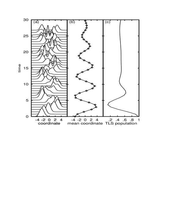
Figure 3.3: Preparation of superpositional state. The HO with $\omega_{0}$ is coupled to a single TLS ($\omega_{\rm TLS}=1.01\omega_{0}$), with coupling $g=0.2\omega_{0}$. Initially the HO is prepared in a coherent state at $Q_{0}=2.5$, the TLS in the excited state. The time axis shows dimensionless time $\omega_{0}t$. (a) Evolution of the HO wave packet $P(Q,t)$. (b) Mean value of the HO coordinate. (c) Population of the TLS.

In this subsection we illustrated a possible method to create a superpositional state (3.1) of a resonator field mode. The preparation of a motional state of a trapped ion in the state  (3.1) is reported in Ref. [77], while the excitation of the molecular vibration in this state by two short laser pulses is discussed in Refs. [78, 79]. In the next subsection we calculate how the superpositional states evolve in time.

3.4.3 Superposition of two coherent states. Decoherence

For the initial superposition of two coherent states (3.1) the normally ordered characteristic function Eq. (3.12) consists of four terms:

$$F\left(\lambda,\lambda^{*},0\right)=N^{-2}\left[F_{\alpha^{*},\alpha}+F_{-\alpha^{*},-\alpha}+e^{-2\left|\alpha\right|^{2}}\left(e^{{{i}}\phi}F_{\alpha^{*},-\alpha}+e^{-{{i}}\phi}F_{-\alpha^{*},\alpha}\right)\right]$$ (3.39)

with $F_{\alpha,\beta}=e^{\alpha\lambda-\beta\lambda^{*}}$. The first terms describe the mixture of two coherent states, $\left|\alpha\right\rangle\left\langle\alpha\right|+\left|-\alpha\right\rangle\left\langle-\alpha\right|$. The last two terms correspond to a quantum interference, i.e., they reflect the coherent properties of the superposition. In accordance with Eqs. (3.18)-(2.20) and the equation of motion (3.2) of the RDM this initial state evolves as

$$P\left(Q,t\right)=\frac{1}{N^{2}}\left[P^{\left(\alpha^{*},\alpha\right)}\left(Q,t\right)+P^{\left(-\alpha^{*},-\alpha\right)}\left(Q,t\right)\right]+P_{\rm int}\left(Q,t\right)$$ (3.40)

with the interference term

$$P_{\rm int}\left(Q,t\right)=\frac{1}{N^{2}}e^{-2\left|\alpha\right|^{2}}\left[e^{{{i}}\phi}P^{\left(\alpha^{*},-\alpha\right)}\left(Q,t\right)+e^{-{{i}}\phi}P^{\left(-\alpha^{*},\alpha\right)}\left(Q,t\right)\right]$$ (3.41)

where $P^{\left(\alpha,\beta\right)}\left(Q,t\right)$ is given by Eq. (3.24) with

$$Q^{\left(\alpha^{*},\alpha\right)}\left(t\right)=-Q^{\left(-\alpha^{*},-\alpha\right)}\left(t\right)=2\Re\left[\alpha z(t)\right]e^{-\gamma t},$$ (3.42)

$$Q^{\left(\alpha^{*},-\alpha\right)}\left(t\right)=-Q^{\left(-\alpha^{*},\alpha\right)}\left(t\right)=2{{i}}{\Im}\left[\alpha z\left(t\right)\right]e^{-\gamma t}.$$ (3.43)

$V\left(t\right)$ and $z\left(t\right)$ are defined by Eqs. (3.28)-(3.29). Rewriting the real part of Eq. (3.41) we finally obtain

$$P_{\rm int}\left(Q,t\right) = \frac{1}{N^{2}}\frac{1}{\sqrt{\pi V\left(t\right)}}\exp\left(-2\left|\alpha\right|^{2}+\frac{4\left\{{\Im}\left[\alpha z(t)\right]\right\}^{2}e^{-2\gamma t}-Q^{2}}{4V(t)}\right)$$

$$\times\Biggl{.}\cos\left\{\phi-Q\frac{{\Im}[\alpha z(t)]}{V(t)}e^{-\gamma t}\right\}.$$

 

Figure 3.4: Time evolution of the superposition of coherent states for $\omega=1$, $\gamma=0.01\omega$, $n=0$, $\alpha=2$, $\phi=\frac{\pi}{2}$.

Figure 3.4 illustrates, how the superpositional state (3.1) evolves in time in accordance with Eq. (3.40). It follows from Eq. (3.4.3), that the interference term describing quantum coherence in the system is only significant when

$$\frac{\left\{{\Im}\left[\alpha z\left(t\right)\right]\right\}^{2}}{V\left(t\right)}e^{-2\gamma t}\approx 2\left|\alpha\right|^{2}.$$ (3.45)

This is true for $\gamma t\ll 1$, and moreover, when the two wave packets of the state (3.1) come close together (i.e., at the moment when $z\left(t_{i}\right)\approx{{i}}$). Expanding Eq. (3.45) into a series at these points and taking into account $\gamma t_{i}\ll 1$, it is easy to see that

$$P_{\rm int}\sim\exp\left(-2\left|\alpha\right|^{2}+\frac{\left\{{\Im}\left[\alpha z\left(t_{{i}}\right)\right]\right\}^{2}}{V\left(t_{i}\right)}\left(1-2\gamma t_{i}\right)\right).$$ (3.46)

The decoherence is due to two reasons: The spreading $V\left(t_{i}\right)=1/2+\Delta V\left(t_{{i}}\right)n$ of the wave packet due to thermal excitations by the bath, and amplitude decoherence. The latter means, that even for the case $n=0$ and ${\Im}\left(\alpha z\left(t_{i}\right)\right)=\left|\alpha\right|$ quantum interference disappears exponentially with the rate

$$t_{\mathrm{dec}}^{-1}\simeq 2\left|\alpha\right|^{2}\gamma$$ (3.47)

This result obtained by Zurek [16] is the main reason why quantum interference is difficult to observe in the mesoscopic and macroscopic world. For example, a physical system with mass 1g in a superposition state with a separation of 1cm shows a ratio of relaxation and decoherence time scales of $10^{40}$. Even if our measuring device is able to reflect the quantum properties of the microsystem, nevertheless objectification [121] occurs due to the coupling between the meter and the environment. The fundamental result of Eq. (3.47) is obtained no matter which approach is used, e.g. the RWA or Zurek’s pointer basis approach or the self-consistent description of the present work. However, the time dependence of the superposition terms of the distribution of Eq. (3.4.3) differs a little bit, which can be seen in Fig. 3.5. As quantum interference is more sensitive, we have used it for comparison of three different approaches to the present problem.

 

Figure 3.5: Time dependence of $P_{\rm int}\left(Q,t\right)$ for $\omega=1$, $\gamma=0.25\omega$, $n=0.4$, $\alpha=2$, $\phi=0$, $Q_{0}=0$. The solid line represents the case Eq. (3.28), the diamonds represent RWA, the bullets represent earliest-time analysis Eq. (3.27).

Figure 3.5 shows the difference between the time evolutions, which result from Eq. (3.27), from Eq. (3.28), and from the corresponding result of the RWA approach.

These differences arise due to the fact that during the relaxation there is no constant pointer basis for all steps of the evolution. As follows from Eqs. (3.10) and (3.2), this basis changes from the position eigenstate basis in Eq. (3.10) to the more complicated basis in Eq. (3.2).

3.4.4 Partial conservation of superposition

As the interference term (3.4.3) of the wave packet decays inevitably, it is difficult to observe the effects mentioned in subsection 3.4.2. The decoherence determines, e. g., the main requirement to the potential elements of quantum computers: the decoherence time should be smaller than the computation time [104]. One should find a system maximally isolated from an environment or increase the decoherence time artificially. One could prolong the coherent interval of the evolution by increasing the number of information transfer channels [122], by feedback methods [123], or by so-called passive methods [124]. Here we discuss in detail one more method of coherence preserving, namely organization of interaction with the environment [16, 125, 126]. The idea of this method is to choose the system or the regime of system evolution which ensures a specific type of system-bath coupling, sometimes a nonlinear one. The linear coupling (3.2) to $A=a^{+}+a$ corresponds to the resonant exchange of quanta between system and bath. A coupling to the number of phonons used in description of a trapped ion [126] and of exciton evolution in molecular crystals [53] describes the bath-induced modulation of the system transition frequency. A coupling of the form $A=(a+\alpha)(a-\alpha)$ is discussed in Ref. [125] and Glauber’s generalized annihilation operator [127, 128]

$$A=a\exp{\left({{i}}\pi a^{+}a\right)}$$ (3.48)

in Ref. [123]. An exotic coupling operator $a\left(a^{+}a-\left\langle a^{+}a\right\rangle\right)$ is discussed in Ref. [126].

Figure 3.6: Schematic presentation of the two-quanta process.

In Zurek’s ansatz [16] the eigenstates $\left|\psi\right>_{A}$ of the coupling operator $A$ (pointer states) are not perturbed by the interaction with the reservoir. For the linear coupling (3.2) and high temperature limit $n\approx n+1$ in Eq. (3.2) such “pointer states” are represented by eigenstates of the coordinate operator [16], namely coherent states. In our approach they evolve in time. For the operator (3.48) the eigen- and, respectively, pointer states coincide with the superpositional states $\left|\alpha,\pi\right>$ given by Eq. (3.1). This coupling preserves the superposition from decoherence, but it is rather difficult to find an experimental system that provides such type of coupling to the environment. We consider a less exotic one, when the majority of the bath modes are not equal in frequency with the selected system, so that loss of amplitude and phase must be delayed. As a simplest example we take the quantum system surrounded by HOs with frequencies doubled to that of the system $\omega_{\xi}=2\omega$ as shown in Fig. 3.6. Although this is still a resonance situation, it leads to unusual behavior compared to the usual case $\omega_{\xi}=\omega$, discussed above. Describing it in RWA we rewrite the interaction (3.2)

$$H_{\rm SE}=\hbar\sum_{\xi}K_{\xi}\left[b^{+}_{\xi}a^{2}+b_{\xi}(a^{+})^{2}\right],$$ (3.49)

as discussed in Ref. [85]. Applying the evolution operator (2.6) we obtain again Eq. (3.3) for the RDM $\sigma$ of the selected system, but with some changes of the relaxational part (3.4)

$$L\sigma = \Gamma(n_{\xi}+1)\left\{\left[a^{2}\sigma,(a^{+})^{2}\right]+\left[(a^{+})^{2},\sigma a^{2}\right]\right\}$$ (3.50)

$$+ \Gamma n_{\xi}\left\{\left[(a^{+})^{2}\sigma,a^{2}\right]+\left[a^{2},\sigma(a^{+})^{2}\right]\right\},$$

where $\Gamma=\pi K_{\xi}^{2}g_{\xi}$ is the decay rate of the vibrational amplitude. Here, the number of quanta in the bath mode $n_{\xi}$, the coupling function $K_{\xi}$, and the density of bath states $g_{\xi}$ are evaluated at $\omega_{\xi}=2\omega$. An analogous equation was derived in Ref. [129]. The zero temperature limit was used in Ref. [85].

In the basis of eigenstates $\left|n\right\rangle$ of the unperturbed oscillator the master eq. (3.50) contains only linear combinations of terms as $\sigma_{m,n}=\left\langle m\right|\sigma\left|n\right\rangle$, $\sigma_{m+2,n+2}$, and $\sigma_{m-2,n-2}$. It distinguishes even and odd initial states of the system. The odd state $\left|1\right\rangle$ cannot relax to the ground state $\left|0\right\rangle$, but the even state $\left|2\right\rangle$ can.

Figure 3.7: Influence of different baths. Evolution of the coherent state: Mean value of the coordinate, for $Q_{0}=-2.2$. Diamonds: system coupled to the bath with $\omega_{\xi}=\omega$, $\gamma=0.15\omega$. Solid line: system coupled to the bath with $\omega_{\xi}=2\omega$, $\Gamma=0.5\omega$.

The evolution of the system from different initial conditions was simulated numerically. The equations of motion of the DM elements are integrated using a fourth-order Runge-Kutta algorithm with stepsize control. To make the set of differential equations a finite one we restrict the number of levels by $m,n\leq 20$.

We show the time dependence of the mean value of the coordinate in Fig. 3.7. The mean value in the usual case $\omega_{\xi}=\omega$ decreases with a constant rate. The same initial value of the system coupled to a bath with $\omega_{\xi}=2\omega$ shows a fast decrement in the first stage and almost no decrement afterwards.

 

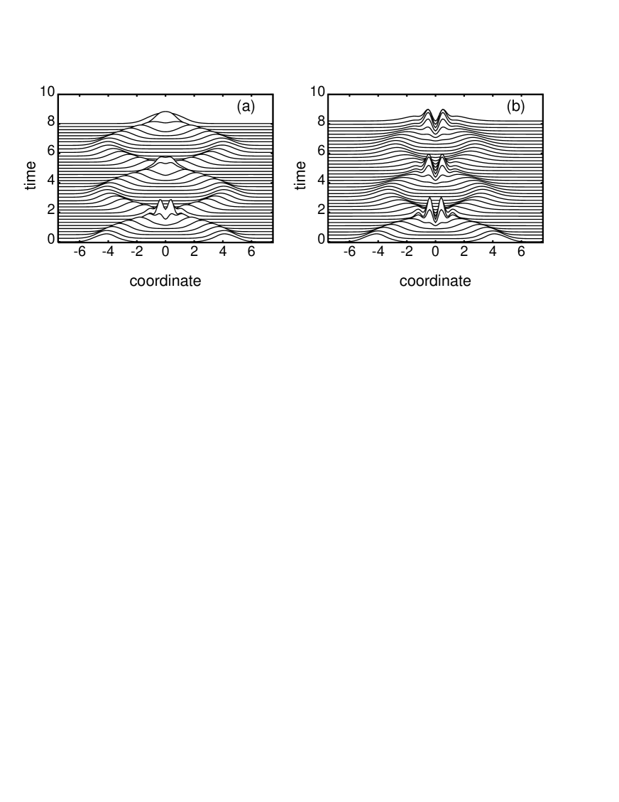
Figure 3.8: Influence of different baths. (a) Time evolution of the superposition of coherent states with initial separation $2Q_{0}=8$ for $\omega_{\xi}=\omega=1$, $\gamma=0.005\omega$, $n=1.36$. (b) Same as (a), but for $\omega_{\xi}=2\omega$ with $\Gamma=0.005\omega$, $n_{\xi}=0.5$.

At temperature $k_{B}T=2\hbar\omega/{\rm ln}3$, corresponding to $n(2\omega)=0.5$, we have simulated the evolution of the same superpositional states for $\omega_{\xi}=\omega$ and for $\omega_{\xi}=2\omega$, presented in Fig. 3.8(a) and 3.8(b). For $\omega_{\xi}=\omega$ the quantum interference disappears already during the first period, while the amplitude decreases only slightly. The bath with $\omega_{\xi}=2\omega$ leaves the interference almost unchanged, although a fast decrease of the amplitude occurs. Therefore, it partially conserves the quantum superpositional state.

3.5 Summary

Starting from von Neumann’s equation for a HO interacting with the environment modeled by a set of independent HOs we derived a non-Markovian master equation, which has been solved analytically. For two types of the bath with maximum of the spectral density near the system frequency and near the double of the system frequency and for two different initial states, namely a coherent state and a superposition of coherent states, the wave packet dynamics in coordinate representation have been analysed. It has been shown that wave packet dynamics demonstrates either ”classical squeezing” and the decrease of the effective vibrational oscillator frequency due to the phase-dependent interaction with the bath, or a time-dependent relaxation rate, distinct for even and odd states, and partial conservation of quantum superposition due to the quadratic interaction with the bath. The decoherence also shows differences compared to the usual damping processes adopting RWA and to the description using the pointer basis for decoherence processes. We conclude that there is no permanent pointer basis for the decay. There are two universal stages of relaxation: the coherence stage and the Markovian stage of relaxation, both having different pointer bases. We believe that the proposed method can be applied for other initial states and different couplings with the environment in real existing quantum systems, which is important in the light of recent achievements in single molecule spectroscopy, trapped ion states engineering, and quantum computation.

Chapter 4 Electron Transfer via Bridges

The present chapter deals with an important and quite difficult problem - the mathematical modeling of ET. The purpose of our investigation is, at the one hand, to present a simple, analytically solvable model based on the RDM formalism [130, 73] and to apply it to a porphyrin-quinone complex which is taken as a model system for the reaction centers in bacterial photosynthesis, and on the other hand, to compare this model with another one, which below we call the vibronic model.

Before the description of these models and mathematical approaches some brief review of the ET problem in experimental and theoretical contexts is represented in section 4.1. In section 4.2 we introduce the model of a molecular aggregate where only electronic states are taken into account because it is assumed that the vibrational relaxation is much faster than the ET. This model is referred to as the tight-binding (TB) model or model without vibrations below. The properties of an isolated aggregate are modeled in subsection 4.2.1, as well as the static influence of the environment. The dynamical influence of bath fluctuations is discussed and modeled by a heat bath of HOs in subsection 4.2.2. The RDMEM describing the excited state dynamics of the porphyrin aggregate is described in subsection 4.2.3 and compared with an analogous equation of Haken, Strobl, and Reineker (HSR) [53, 131, 132, 133] in appendix A. In subsection 4.2.4 the system parameter dependence on the solvent dielectric constant is discussed for different models of solute-solvent interaction. In Subsection 4.3 system parameters are determined. The methods and results of the numerical and analytical solutions of the RDMEM are presented in subsection 4.4.

The dependencies of the transfer rate and final acceptor population on the system parameters are given for the numerical and analytical solutions in subsection 4.5.1. The analysis of the physical processes in the system is also performed there. In subsection 4.5.2 we discuss the dependence of the transfer rate on the solvent dielectric constant for different models of solute-solvent interaction and compare the calculated transfer rates with the experimentally measured ones. The advantages and disadvantages of the presented method in comparison with the method of Davis et al. [10] are analysed in subsection 4.5.3.

The vibronic model is described in section 4.6. In this case one pays attention to the fact that experiments in systems similar to the one discussed here show vibrational coherence [134, 135]. Therefore a vibrational substructure is introduced for each electronic level within a multi-level Redfield theory [136, 137]. The comparison of this model with the first one is done in section 4.7. At the end of the chapter the achievements and possible extensions of this consideration are discussed. Unless otherwise stated SI units are used.

4.1 Introduction to the electron transfer problem

Long-range ET is a very actively studied area in chemistry, biology, and physics; both in biological and synthetic systems. Of special interest are systems with a bridging molecule between donor and acceptor. For example the primary step of charge separation in the bacterial photosynthesis takes place in such a system [6].

4.1.1 Mechanism of the electron transfer in bridge systems

It is known that the electronic structure of the bridge component in donor-bridge-acceptor systems plays a critical role [138, 139]. Change of a building block of the complex [8, 140, 141] or change of the environment [140, 142] can modify which mechanism is mainly at work: coherent superexchange or incoherent sequential transfer. Here the bridge energy stands for the energy of the state with electron localized on the bridge, not the locally excited electronic state of the bridge. When the bridge energy is much higher than the donor and acceptor energies, the bridge population is close to zero for all times and the bridge site just mediates the coupling between donor and acceptor. This mechanism is called superexchange and was originally proposed by Kramers [143] to describe the exchange interaction between two paramagnetic atoms spatially separated by a nonmagnetic atom. In the case when donor and acceptor as well as bridge energies are closer than $\sim k_{{\rm B}}T$ or the levels are arranged in the form of a cascade, the bridge site is actually populated and the transfer is called sequential. The interplay between these two types of transfer has been investigated theoretically in various publications [144, 145, 146]. Actually, there is still a discussion in the literature whether sequential transfer and superexchange are limiting cases of one process [144] or whether they are two processes which can coexist [6]. To clarify which mechanism is present in an artificial system one can systematically vary both energetics of donor and acceptor and electronic structure of the bridge. In experiments this is done by substituting parts of the complexes [140, 141, 147] or by changing the polarity of the solvent [140]. Also the geometry and size of the bridging block can be varied, and in this way the length of the subsystem through which the electron has to be transfered [147, 148, 149, 150] can be changed.

Superexchange occurs due to coherent mixing of the three or more states of the system [151, 152]. The transfer rate in this channel depends algebraically on the differences between the energy levels [8, 9] and decreases exponentially with increasing length of the bridge [150, 152]. When incoherent effects such as dephasing dominate, the transfer is mainly sequential [11, 150], i. e., the levels are occupied mainly in sequential order [5, 11, 12, 140]. The dependence on the differences between the energy levels is exponential [8, 9]. An increase of the bridge length induces only a small reduction in the transfer rate [145, 148, 150, 152]. This is why sequential transfer is the desired process in molecular wires [150, 153].

4.1.2 Known mathematical theories

In the case of coherent superexchange the dynamics is mainly Hamiltonian and can be described on the basis of the Schrödinger equation. The physically important results can be obtained by perturbation theory [13, 154] and, most successfully, by the semiclassical Marcus theory [155]. The complete system dynamics can directly be extracted by numerical diagonalisation of the Hamiltonian [150, 156]. In case of sequential transfer the environmental influence has to be taken into account. There are quite a few different ways how to include the influence of an environment modeled by a heat bath. The simplest phenomenological descriptions of the environmental influence are based on the Einstein coefficients or on the imaginary terms in the Hamiltonian [157, 158], as well as on the Fokker-Planck or Langevin equations [157, 158]. The most accurate but also numerically most expensive way is the path integral method [157]. This has been applied to bridge-mediated ET especially in the case of bacterial photosynthesis [159]. Bridge-mediated ET has also been investigated using Redfield theory [12, 145], by propagating a DM in Liouville space [11] and other methods (e. g. [152, 156, 160]). In most of these methods vibrations are taken into account.

The master equation which governs the DM evolution as well as the appropriate relaxation coefficients can be derived from such basic information as system-environment coupling strength and spectral density of the environment [24, 73, 130, 136, 161, 162]. In the model without vibrations the relaxation is introduced in a way similar to Redfield theory but in site representation instead of eigenstate representation. A discussion of advantages and disadvantages of site versus eigenstate representation has been given elsewhere [163]. The equations obtained are similar to those of Ref. [10] where relaxation is introduced in a phenomenological fashion but only a steady-state solution is found in contrast to the model used in this chapter. In addition, the present model is applied to a concrete system. A comparison of the ET time with the bath correlation time allows us to regard three time intervals of system dynamics: the interval of memory effects, the dynamical interval, and the kinetic, long-time interval [53]. In the framework of DM theory one can describe the ET dynamics in all three time intervals. However, often it is enough to find the solution in the kinetic interval for the explanation of experiments within the time resolution of most experimental setups, as has been done in Ref. [10, 164]. The master equation is analytically solvable only for simple models, for example [158, 165]. Most investigations are based on the numerical solution of this equation [11, 136, 137, 145, 161, 166]. However, an estimation can be obtained within the steady-state approximation [10, 167].

We should underline here that the RDMEM contains the coherent dynamics term and, therefore, is able to describe the SE mechanism. This fact has been recognized and successfully used to describe the reactions with dominance of superexchange in a various publications [10, 12, 145]. Davis et al. [10] have explicitly rederived the McConnel analytical expression for superexchange using the RDMEM technique. based on the ability of the diabatic RDMEM to account for the coherent effects we apply the RDMEM formalism to describe the ET in a real system where superexchange most probably takes place.

4.1.3 Porphyrin-quinone complex as model for electron transfer

The photoinduced ET in the supermolecule consisting of three sequentially connected molecular blocks, i. e., donor (D), bridge (B), and acceptor (A), is under consideration throughout this chapter. D is not able to transfer its charge directly to A because of their spatial separation. D and A can exchange their charges only through B. In the present investigation, the supermolecular system consists of free-base of tetraphenylporphyrin (${\rm H_{2}P}$) as D, zinc-tetraphenylporphyrin (${\rm ZnP}$) as B, and p-benzoquinone as A [140] as shown in Fig. 4.1.

 

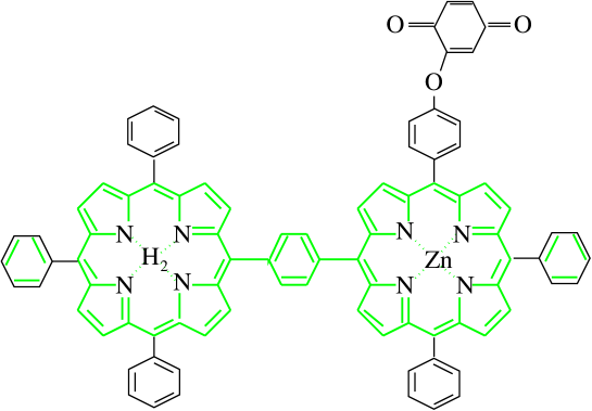
Figure 4.1: Chemical structure of ${\rm H_{2}P-ZnP-Q}$.

4.2 Model without vibrations

In each of those molecular blocks shown in Fig. 4.1 we consider only two molecular orbitals, the lowest unoccupied molecular orbital (LUMO) and the highest occupied molecular orbital (HOMO) [168]. Each of the above-mentioned orbitals can be occupied by an electron or not, denoted by $|1\rangle$ or $|0\rangle$, respectively. This model allows to describe four states of the molecular block (e. g. D), the neutral ground state $|1\rangle_{\rm HOMO}|0\rangle_{\rm LUMO}$ (${\rm D}$), the neutral excited state $|0\rangle_{\rm HOMO}|1\rangle_{\rm LUMO}$ (${\rm D^{*}}$),, the positively charged ionic state $|0\rangle_{\rm HOMO}|0\rangle_{\rm LUMO}$ (${\rm D^{+}}$),, and the negatively charged ionic state $|1\rangle_{\rm HOMO}|1\rangle_{\rm LUMO}$ (${\rm D^{-}}$),. Below a small roman index denotes the molecular orbital ($m=0$ - HOMO, $m=1$ - LUMO), while a capital index denotes the molecular block ($M{}=1$ - D, $M{}=2$ - B, $M{}=3$ - A). A state of the supermolecule can be described as the direct product of the molecular block states. $c^{+}_{M{}m}=|1\rangle_{M{}m}\langle 0|_{M{}m}$, $c_{M{}m}=|0\rangle_{M{}m}\langle 1|_{M{}m}$, and $\hat{n}_{M{}m}=c^{+}_{M{}m}c_{M{}m}$ describe the creation, annihilation, and number of electrons in orbital ${M{}m}$, respectively, while $\hat{n}_{M}{}=\sum_{m}\hat{n}_{M{}m}$ gives the number of electrons in a molecular block. The number of particles in the whole supermolecule is conserved $\sum_{M}{}{\hat{n}}_{M}{}=const$. Some of the electronic states of the molecular aggregate are shown in Fig. 4.2.

 

Figure 4.2: Schematic presentation of the energy levels in the ${\rm H_{2}P}-{\rm ZnP}-{\rm Q}$ complex. The three states in the boxes play the main role in ET which can happen either sequentially or by a superexchange mechanism. Dashed lines refer to a sequential transfer, curved solid line to superexchange, dot-dashed to an energy transfer followed by charge transfer, dotted line optical excitation, and straight solid lines either fluorescence or non-radiative recombinations.

Each of the electronic states has its own vibrational substructure. As a rule for the porphyrin containing systems the time of vibrational relaxation is found to be two orders of magnitude faster than the characteristic time of the ET [169]. Because of this we assume that only the vibrational ground states play a role in ET, and we do not include the vibrational structure. A comparison of the models with and without vibrational substructure will be given in section 4.6.

4.2.1 System part of the Hamiltonian

For the description the charge transfer and other dynamical processes in the system placed in a dissipative environment we use the common form of the Hamiltonian (2.1) where $\hat{H}^{\rm S}$ is the Hamiltonian of the supermolecule, $\hat{H}^{\rm E}$ the Hamiltonian of the dissipative bath, and $\hat{H}^{\rm SE}$ describes their interaction. As mentioned in the introduction we are mainly interested in the kinetic limit of the excited state dynamics here. For this limit we assume that the relaxation of the solvent takes only a very short time compared to the timescale of interest for the system. Here the effect of the solvent is considered to be twofold. On the one hand the system states are shifted in energy. This static effect is state-specific and discussed below. On the other hand the system dynamics is perturbed by the solvent state fluctuations, which are independent of the system states. The interaction Hamiltonian shall only reflect the dynamical influence of the fluctuations leading to dissipative processes as discussed in the next subsection.

The static influence of the solvent is determined by the relaxed value of the solvent polarization and in general also includes the non-electrostatic contributions such as van-der-Waals attraction and short-range repulsion [170, 171]. It is included into the system state energies and modeled as a function of the dielectric constant of the solvent. The static influence induces a change in the energy levels [172],

$$\hat{H}^{\rm S}=\hat{H}_{0}+\hat{H}_{\rm es}+\hat{V},$$ (4.1)

where the energy of free and noninteracting blocks $\hat{H}_{0}$ corresponds to the energy of independent electrons in the field of the ionic nuclei. The term $\hat{H}_{\rm es}$ denotes the state-selective electrostatic interaction within a molecular aggregate depending on the static dielectric constant $\epsilon_{\rm s}$ of the solvent and $\hat{V}$ the inter-block hopping. It is assumed that the hopping $\hat{V}$ within the supermolecule is affected by the surroundings as discussed in subsection 4.2.4.

The energies of the independent electrons can be calculated by $\hat{H}_{0}=\sum_{M{}m}E_{M{}m}\hat{n}_{M{}m}$, where $E_{M{}m}$ denotes the energy of orbital $M{}m$ in the independent particle approximation [4, 173]. We introduce such a simplified model to be able to calculate the energies of ionic molecular blocks e. g. ${\rm D}^{-}$. For each molecular block a fitting parameter $A_{M}$ is introduced which is used to reproduce the ground state-excited state transition e. g. ${\rm D}\rightarrow{\rm D}^{*}$. Because these transitions change only a little for different solvents [140], the parameters $A_{M}$ are assumed to be solvent-independent. This is why we do not scale $\hat{H}_{0}$. In order to determine $E_{M{}m}$ one starts from fully ionized double bonds in each molecular block [173], calculates the one-particle states in the field of the ions in site representation and fills each of these orbitals with two electrons starting from the lowest orbital;

$$E_{Mm} = \sum_{s=-\frac{N_{M}}{2}-d_{M}+{\rm int}\left(\frac{d_{M}}{2}\right)}^{-\frac{N_{M}}{2}+{\rm int}\left(\frac{d_{M}}{2}\right)}\left(\tilde{E}_{M}{}-2A_{M}{}\cos{\frac{2\pi s}{N_{M}}}\right)$$

$$+ m\left(\tilde{E}_{M}-2A_{M}\cos{\left\{\frac{2\pi}{N_{M}}\left[-\frac{N_{M}}{2}+{\rm int}\left(\frac{d_{M}}{2}\right)+1\right]\right\}}\right).$$

Here $N_{M}{}$ and $d_{M}{}$ are the total number of bonds and number of double bonds, respectively, in the porphyrin rings ($M=1$, $2$. For $M=3$, i. e., the quinone (Q), see Sect. 4.3.). The energy shift $\tilde{E}_{M}{}$ is chosen such that the neutral complex has zero energy. $A_{M}{}$ denotes the energy of hopping between two neighboring sites of the $M{}$th molecular block. The function ${\rm int}()$ in Eq. (4.2.1) denotes the integer part of a real number. In a similar way, by exciting, removing, or adding the last electron to the model system, one obtains the energy of the excited, oxidized, or reduced molecular block in the independent particle approximation.

Below we apply Eqs. (2.27)-(2.5) to the problem of evolution of a single charge-transfer exciton states in the system. In this case the number of states coincides with the number of sites in system:

$$\{Mm\}\rightarrow\mu.$$ (4.3)

The next contribution to the system Hamiltonian is the inter-block hopping term

$$\hat{V}=\sum_{M{}N}v_{\mu{}\nu}(\hat{V}^{+}_{\mu{}\nu}+\hat{V}_{\mu{}\nu})\left[(\hat{n}_{M}{}-1)^{2}+(\hat{n}_{N}-1)^{2}\right].$$

It includes the hopping operator between two LUMO states

$$\hat{V}_{\mu\nu}=c^{+}_{M1}c_{N1},$$ (4.4)

as well as the corresponding intensities $v_{\mu{}\nu}$, i.e., the coherent coupling between different states of the system. We assume $v_{13}=0$ because there is no direct connection between donor and acceptor. The scaling of $v_{\mu\nu}$ for different solvents is discussed in subsection 4.2.4.

Figure 4.3: Schematic view of the multiple cavities model

The electrostatic interaction $\hat{H}_{\rm es}$ scales like energies of a system of charges in a single or in multiple cavities surrounded by a medium with dielectric constant $\epsilon_{\rm s}$ according to the classical reaction field theory [174]. Here we consider two models of scaling. In the first model each molecular block of the aggregate is in the individual cavity as shown in Fig. 4.3. For this case the electrostatic energy reads

$$\hat{H}_{\rm es}=S^{H}(\epsilon_{\rm s})\left(\hat{H}_{\rm el}+\hat{H}_{\rm ion}\right).$$ (4.5)

Here the function $S^{H}(\epsilon_{\rm s})$ describes the scaling of the electrostatic energy with the static dielectric constant $\epsilon_{\rm s}$ of the solvent. The term

$$\hat{H}_{\rm el}=\sum_{\mu}{}(\hat{n}_{\mu}{}-1)\frac{e^{2}}{4\pi\epsilon_{0}}\frac{1}{r_{\mu}{}}$$ (4.6)

takes the electron interaction into account while bringing an additional charge onto the block $\mu{}$ and thus describes the energy to create an isolated ion. This term depends on the characteristic radius $r_{\mu}{}$ of the molecular block. The interaction between the ions

$$\hat{H}_{\rm ion}=\sum_{\mu}{}\sum_{\nu}(\hat{n}_{\mu}{}-1)(\hat{n}_{\nu}-1)\frac{e^{2}}{4\pi\epsilon_{0}}\frac{1}{r_{\mu{}\nu}}$$ (4.7)

depends on the distance between the molecular blocks $r_{\mu{}\nu}$. Both distances $r_{\mu}{}$ and $r_{\mu{}\nu}$ are also used in the Marcus theory [155]. The term $H_{\rm el}+H_{\rm ion}$ reflects the interaction of charges inside the aggregate which are compensated by the reaction field according to the Born formula [175]

$$S^{H}=1+\frac{1-\epsilon_{\rm s}}{2\epsilon_{\rm s}}=\frac{1}{2\epsilon_{\rm s}}+\frac{1}{2}.$$ (4.8)

In the second model sketched in Fig. 4.4, considering the aggregate as an single object placed in a cavity of constant radius one has to use the Onsager term [175]. This term is state selective, i.e., it gives a contribution only for the states with nonzero dipole moment, i.e., charge separation. Defining the static dipole moment operator as $\hat{\vec{p}}=\sum\limits_{\mu{}\nu}(\hat{n}_{\mu}{}-1)(\hat{n}_{\nu}-1)\vec{r}_{\mu{}\nu}e$ we obtain the Onsager term: $\hat{H}_{\rm es}=S^{H}\hat{H}_{\rm dip}$, where $\hat{H}_{\rm dip}=\frac{\hat{\vec{p}}^{2}}{r_{13}}$,

$$S^{H} = \frac{1-\epsilon_{\rm s}}{2\epsilon_{\rm s}+1}.$$ (4.9)

Figure 4.4: Schematic view of the single cavity model

So, the physical meaning of both scalings is briefly summarized as follows: Born-Marcus scaling corresponds to three cavities in the dielectric, each containing one molecular block of the aggregate. The energy scales with the Born formula (4.8). Onsager scaling Eq. (4.9) reflects the naive idea that the whole supermolecule is placed in a single cavity.

4.2.2 Microscopic motivation of the system-bath interaction and the thermal bath

One can express the dynamic part of the system-bath interaction as

$$\hat{H}^{\rm SE}=-\int d^{3}\vec{r}\sum_{\mu{}\nu}\hat{\vec{D}}_{\mu{}\nu}(\vec{r})\cdot{}\Delta\hat{\vec{P}}(\vec{r}).$$ (4.10)

Here $\hat{\vec{D}}_{\mu{}\nu}(\vec{r})$ denotes the field of the electrostatic displacement at point $\vec{r}$ induced by the system transition dipole moment $\hat{\vec{p}}_{\mu{}\nu}=\vec{p}_{\mu\nu}(\hat{V}^{+}_{\mu{}\nu}+\hat{V}_{\mu{}\nu})$ [158]

$$\hat{\vec{D}}_{\mu{}\nu}(\vec{r})=\frac{1}{4\pi\epsilon_{0}}\left[\frac{3(\hat{\vec{p}}_{\mu{}\nu}\cdot{}\vec{r})\vec{r}}{r^{5}}-\frac{\hat{\vec{p}}_{\mu{}\nu}}{r^{3}}\right].$$ (4.11)

The field of the environmental polarization s denoted as $\hat{\vec{P}}(\vec{r})=\sum_{n}\delta(\vec{r}-\vec{r}_{n})\hat{\vec{d}}_{n}$, where $\hat{\vec{d}}_{n}$ is the $n$th dipole of the environment and $\vec{r}_{n}$ its position. Only fluctuations of the environment polarization $\Delta\hat{\vec{P}}(\vec{r})$ influence the system dynamics. Averaged over the angular dependence the interaction reads [172]

$$\hat{H}^{\rm SE}=-\sum\limits_{\mu{}\nu n}\frac{1}{4\pi\epsilon_{0}}\left(\frac{2}{3}\right)^{\frac{1}{2}}\frac{|\hat{\vec{p}}_{\mu\nu}|\Delta|\hat{\vec{d}_{n}}|}{|\vec{r}_{n}|^{3}}.$$ (4.12)

The dynamical influence of the solvent is described with the thermal bath model. The deviation $\Delta\left|\hat{\vec{d}}_{n}\right|$ of $d_{n}$ from its mean value is determined by temperature induced fluctuations. One could couple $\hat{V}_{\mu\nu}$ to $\hat{\vec{d_{n}}}$ or $\Delta\left|\hat{\vec{d}}_{n}\right|$. But, solvent dipoles interact with each other even in the absence of a supermolecular aggregate. For unpolar solvents described by a set of HOs the diagonalisation of their interaction yields the bath of HOs with different frequencies $\omega_{\lambda}$ and effective masses $m_{\lambda}$.

In the case of a polar solvent the dipoles are interacting rotators as, e. g. used to describe magnetic phenomena [176, 177]. The elementary excitation of each frequency can again be characterised by an appropriate HO. So, we use generalized coordinates of solvent oscillators modes

$$\hat{Q}_{\lambda}=\sqrt{\frac{\hbar}{2m_{\lambda}\omega_{\lambda}}}(\hat{b}_{\lambda}+\hat{b}^{+}_{\lambda})$$ (4.13)

for polar as well as unpolar solvents. The occupation of the $i$th state of the $\lambda$th oscillator is defined by the equilibrium DM $\rho_{\lambda,ij}=\exp{\left(-\frac{\hbar\omega_{\lambda}i}{k_{B}T}\right)}\delta_{ij}$.

All mutual orientations and distances of solvent molecules have equal probability. An average over all spatial configurations is performed. The interaction Hamiltonian (4.12) is written in a form which is bilinear in system and bath operators:

$$\hat{H}^{\rm SE}=\left[\sum_{\mu{}\nu}p_{\mu{}\nu}(\hat{V}_{\mu{}\nu}+\hat{V}^{+}_{\mu{}\nu})\right]\left[\sum_{\lambda}K_{\lambda}(\hat{b}^{+}_{\lambda}+\hat{b}_{\lambda})\right]$$ (4.14)

The coefficients

$$K_{\lambda}=\frac{1}{4\pi\epsilon_{0}}\left(\frac{2}{3}\right)^{\frac{1}{2}}\int\frac{d^{3}\vec{r}}{|\vec{r}|^{3}}e\sqrt{\frac{\hbar}{2m_{\lambda}\omega_{\lambda}}}S^{\rm SE}(\epsilon_{\rm s})$$ (4.15)

depend on properties of the solvent, in particular, the frequencies $\omega_{\lambda}$. The precise determination of these coefficients needs special consideration. Expression (4.12) includes the dipole moment values corresponding to environmental modes and system transitions. The electric field of a dipole in medium is equivalent to the field of an imaginary dipole with a moment depending on the properties of the medium [174]. This influence of the medium is reflected here by the scaling function $S^{\rm SE}$. Explicit expressions for the solvent influence are still under discussion in the literature [170, 171].

4.2.3 Reduced density matrix approach

As usual the bath is given by HOs which describe the irradiative relaxation properties of the system. For the full description of the system one also should include photon modes to describe for example the fluorescence from the LUMO to the HOMO in each molecular block transferring an excitation to the electro-magnetic field with rate $G_{\mu}$ [158]. The rate of the radiative processes is small in comparison to other processes in system. That is why only the irradiative contribution is treated below. The treatment is similar to Redfield theory [24]. For sake of notation and completeness we repeat the most important steps here for our model Hamiltonian.

The irradiative contribution of the system-bath interaction corresponds to energy transfer to the solvent and spreading of energy over vibrational modes of the supermolecule. Applying the RWA to Eq. (4.14) one gets

$$\hat{H}^{\rm SE}=\sum_{\lambda}\sum_{\mu{}\nu}K_{\lambda}p_{\mu{}\nu}\hat{b}^{+}_{\lambda}\hat{V}_{\mu{}\nu}+h.c.,$$ (4.16)

where $K_{\lambda}p_{\mu{}\nu}$ denotes the interaction intensity between the bath mode $b_{\lambda}$ of frequency $\omega_{\lambda}$ and the quantum transition $\mu{}\nu$ between the LUMOs of molecules $\mu{}$ and $\nu$ of frequency $\omega_{\mu{}\nu}=\frac{1}{\hbar}\left(E_{\mu}-E_{\nu}\right)$.

The dynamics of the system plus bath cannot be calculated due to the huge number of degrees of freedom. Therefore one uses the RDMEM technique. Below we assume that the coherent and dissipative dynamics can be represented by the independent terms of the RDMEM. This assumption is applicable if $v_{\mu\nu}\ll\omega_{\mu\nu}$.

Here we use the RDMEM (2.5) derived in section 2.5. Here we treat the system $p_{\mu\nu}$ and bath $K_{\lambda}$ contributions to the system-bath coupling separately. That is why we define the spectral density of bath modes as $J(\omega)=\pi\sum_{\lambda}K_{\lambda}^{2}\delta(\omega-\omega_{\lambda})$ and the relaxation constant for Eq. (2.5)

$$\Gamma_{\mu\nu}=\hbar^{-2}J(\omega_{\mu{}1\nu 1})p^{2}_{\mu{}\nu}$$ (4.17)

depends on the coupling of the transition $\left|\mu\right>\to\left|\nu\right>$ to the bath mode of the same frequency. Formally, the damping constant depends on the density of bath modes $J$ at the transition frequency $\omega_{\mu\nu}$ and on the transition dipole moments between the system states $p_{\mu{}\nu}$.

For the sake of concrete calculations we write the RDMEM in matrix form. Substituting the expressions for the exciton density $\hat{\sigma}=\sum\limits_{\mu\nu}\sigma_{\mu\nu}\left|\nu\right\rangle\left\langle\nu\right|$, and operators Eq. (4.4) into the relaxation term Eq. (2.5) yields:

$$(L_{\rm RWA}\sigma)_{\kappa\lambda}= 2\delta_{\kappa\lambda}\sum\limits_{\mu}\left\{\Gamma_{\mu\kappa}\left[n(\omega_{\mu\kappa})+1\right]+\Gamma_{\kappa\mu}n(\omega_{\kappa\mu})\right\}\sigma_{\mu\mu}$$ (4.18)

$$-\sum\limits_{\mu}\left\{\Gamma_{\mu\kappa}\left[n(\omega_{\mu\kappa})+1\right]+\Gamma_{\kappa\mu}n(\omega_{\kappa\mu})\right.$$

$$+\left.\Gamma_{\mu\lambda}\left[n(\omega_{\mu\lambda})+1\right]+\Gamma_{\lambda\mu}n(\omega_{\lambda\mu})\right\}\sigma_{\kappa\lambda}.$$

A RDMEM of similar structure was used for the description of exciton transfer by Haken, Strobl, and Reineker in [53, 131, 132, 133, 178]. We present the comparison of these RDMEMs with Eq. (4.18) in appendix A.

For the description of a concrete system the introduced RDMEM (2.27)-(2.5) is used in the matrix form Eq. (4.18) with the use of an index simplification Eq. (4.3). For the sake of convenience of analytical and numerical calculations we replace the relaxation constant $\Gamma_{\mu{}\nu}$ and the population of the corresponding bath mode $n(\omega_{\mu{}\nu})$ with the intensity of dissipative transitions $d_{\mu\nu}=\Gamma_{\mu\nu}|n(\omega_{\mu\nu})|$ between two states, as well as the corresponding dephasings intensity

$$\gamma_{\mu\nu}=\sum_{\kappa}\left(d_{\mu\kappa}+d_{\kappa\nu}\right).$$ (4.19)

With this one can express the RDMEM (4.18) in the form

$$\dot{\sigma}_{\mu\mu} = -i/\hbar\sum_{\nu}(v_{\mu\nu}\sigma_{\nu\mu}-\sigma_{\mu\nu}v_{\nu\mu})+(L\sigma)_{\mu\mu}$$ (4.20)

$$\dot{\sigma}_{\mu\nu} = (-i\omega_{\mu\nu}-\gamma_{\mu\nu})\sigma_{\mu\nu}-i/\hbar v_{\mu\nu}(\sigma_{\nu\nu}-\sigma_{\mu\mu}),$$ (4.21)

where

$$(L\sigma)_{\mu\mu}=-\sum_{\nu}d_{\mu\nu}\sigma_{\mu\mu}+\sum_{\nu}d_{\nu\mu}\sigma_{\nu\nu}.$$ (4.22)

From the manifold of system states we choose the ones which play the essential role in the electron transfer from the donor to acceptor Fig. 4.2. They can be described in terms of single charge transfer exciton and correspond to the index simplification Eq. (4.3). The parameters controlling the transitions between the selected states are discussed in the next section 4.3 and shown explicitly in Fig. 4.5.

 

Figure 4.5: Schematic presentation of the model without vibrational substructure.

4.2.4 Scaling of the relaxation coefficients

The relaxation coefficients $\Gamma_{\mu{}\nu}$ include the second power of the scaling function $\Gamma_{\mu{}\nu}(\epsilon)=\Gamma^{0}_{\mu{}\nu}{S^{\rm SE}}^{2}(\epsilon)$ because one constructs the relaxation term Eq. (2.24) with the second power of the interaction Hamiltonian. The physical meaning of $H^{\rm SE}$ is similar to the interaction of the system dipole with a surrounding media. That is why it is reasonable to use the relevant expressions from the relaxation theory of Onsager and Kirkwood [174] $S^{\rm SB}=\frac{1-\epsilon_{\rm s}}{2\epsilon_{\rm s}+1}$. In the work of Mataga, Kaifu, and Koizumi [179] the interaction energy between the system dipole and the media scales in leading order as

$$S^{\rm SE}=-\left[\frac{2(\epsilon_{\rm s}-1)}{2\epsilon_{\rm s}+1}-\frac{2(\epsilon_{\infty}-1)}{2\epsilon_{\infty}+1}\right],$$ (4.23)

where $\epsilon_{\infty}$ denotes the optical dielectric constant. In a recent paper of Georgievskii, Hsu, and Marcus [170] a connection $J(\omega)=-{\Im}\alpha(\omega)$ between $J(\omega)$ and the generalized susceptibility $\alpha(\omega)$ is introduced and the explicit dependence $\alpha(\omega)$ on the dielectric parameters of the solvent is given. In application to the present work this means that the relaxation coefficient scales like $\Gamma_{\mu{}\nu}={S^{\rm SE}}^{2}\hbar^{-2}J(\omega_{\mu\nu})p^{2}_{\mu{}\nu}$. For example the approximation of spherical molecules gives $\alpha(\omega)\sim\frac{1}{\epsilon_{\rm s}}-\frac{1}{\epsilon_{\omega}}$. We approximate $\epsilon_{\omega}=\epsilon_{\infty}$ here, so $\Gamma\sim\frac{1}{\epsilon_{\rm s}}-\frac{1}{\epsilon_{\infty}}$. In terms of scaling function it can be expressed as

$$S^{\rm SE}=\left(\frac{1}{\epsilon_{\rm s}}-\frac{1}{\epsilon_{\infty}}\right)^{\frac{1}{2}}.$$ (4.24)

As an alternative possibility one can test the case of solvent-independent relaxation coefficient $\Gamma_{\mu{}\nu}=const$, $S^{\rm SE}=1$.

The coherent coupling $v_{\mu\nu}$ between two electronic states scales with $\epsilon_{\rm s}$ and $\epsilon_{\infty}$ too, because a coherent transition in the system is accompanied by a transition of the environment state which is larger for the solvents with larger polarity. Here we involve the concept of reorganization energy from the model with vibrational substructure to account for this effect. For the reorganization energy we take the static part of the system-bath interaction calculated in frames of either individual or multiple cavity model. Here we take the static part ${H^{\rm SE}}^{\rm s}=S^{\rm SE}\left(\hat{H}_{\rm el}+\hat{H}_{\rm ion}\right)$, note that the electronic part of ${H^{\rm SE}}^{\rm s}$ does not scale for the single cavity model. ${H^{\rm SE}}^{\rm s}$ is associated with the so-called reorganization energy. The coherent couplings decrease with increase of ${H^{\rm SE}}^{\rm s}$. For the bath of relatively high frequency HOs (like the $C-C$ stretching vibrations) this scaling can be taken [180] as

$$v_{\mu\nu}=v^{0}_{\mu\nu}\exp{\left[-\left|{\left<\mu\nu|{H^{\rm SE}}^{\rm s}|\mu\nu\right>}\left({2\hbar\omega_{\rm vib}}\right)^{-1}\right|\right]},$$ (4.25)

where $v^{0}_{\mu\nu}$ is the coupling of electronic states of the isolated molecule, $\omega_{\rm vib}$ the leading (mean) environment oscillator frequency. Unless otherwise stated $\omega_{\rm vib}=1500~{}{\rm cm}^{-1}$ is used.

4.3 Model parameters

The dynamics of the system is controlled by the following parameters: energies of system levels $E_{\mu}$, coherent couplings $v_{\mu{}\nu}$, and dissipation intensities $\Gamma_{\mu{}\nu}$. The simplification is that we do not calculate these parameters, exept B state energy, rather take the corresponding experimental values.

The absorption spectra of porphyrins [140] consist of a high frequency Soret band and a low frequency $Q$ band. In the case of ZnP the $Q$ band has two subbands, corresponding to pure electronic $Q(0,0)$ and vibronic $Q(1,0)$ transitions. In the free-base porphyrin ${\rm H_{2}P}$ the reduction of symmetry $D_{4h}\to D_{2h}$ due to the substitution of the central Zn ion by two inner hydrogens induces a splitting of each subband into two, namely $Q^{x}(0,0)$, $Q^{y}(1,0)$ and $Q^{x}(0,0)$, $Q^{y}(1,0)$. So the absorption spectra of ${\rm ZnP}$ and ${\rm H_{2}P}$ consist of two and four bands respectively. In the emission spectra one sees only two bands for each molecule because of cascade intramolecular relaxations: pure electronic and vibronic one.

Table 4.1: Low-energy bands of the porphyrin spectra in ${\rm CH_{2}Cl_{2}}$, from [181]

	Absorption		Emission
	Frequency, ${\rm eV}$	Width, ${\rm eV}$	Frequency, ${\rm eV}$	Width, ${\rm eV}$
${\rm H_{2}P}$	$\nu_{00}^{x}=1.91$	$\gamma_{00}^{x}=0.06$	$\nu_{01}^{x}=1.73$	$\gamma_{01}^{x}=0.05$
${\rm ZnP}$	$\nu_{00}=2.13$	$\gamma_{00}=0.07$	$\nu_{01}=1.92$	$\gamma_{01}=0.05$

Each of the above-mentioned spectra can be represented as a sum of Lorentzians with a good accuracy. The absorption spectrum of the complex ${\rm H_{2}P-ZnP-Q}$ consists of the spectra of the individual ${\rm H_{2}P}$, ZnP, and Q compounds without essential changes. It means that intermolecular interactions in this case do not change the structure of electronic states of the subunits [181]. We consider only the states corresponding to the lowest band of each spectrum to find the parameters of ET. The respective frequencies $\nu$ and widths $\gamma$ are shown in Table 4.1 for ${\rm CH_{2}Cl_{2}}$ as solvent. The width of each band is formed by transitions to different sublevels of the electronic excited states of the aggregate and by the lifetime of these sublevels. In the present model consideration we do not have an excited level substructure, so that we cannot determine the linewidths correctly. Nevertheless we can consider the widths from Table 4.1 as upper limits for the relaxation constants.

On the basis of the given spectral data and taking as reference energy $E_{\rm DBA}=0$ we determine $E_{\rm D^{*}BA}=1/2(\nu_{00}^{x}+\nu_{01}^{x})=1.82$ eV and $E_{\rm DB^{*}A}=2.03~{}{\rm eV}$ (in ${\rm CH_{2}Cl_{2}}$) which allows us to extract the hopping energies $A_{\rm D}=3.11~{}{\rm eV}$, $A^{\rm B}=3.45~{}{\rm eV}$ introduced in Eq. (4.2.1). The excitation spectrum of the quinone lies far from the visible range, in the ultraviolet range. We do not have a precise spectral information about ${\rm Q}$ and, therefore, we do not calculate $A_{\rm A}$. We simply take the energy of the state with charge transfer to ${\rm Q}$ from reference [140]: $E_{\rm D^{+}BA^{-}}=1.42~{}{\rm eV}$. [182]. Further Rempel and coauthors [140] estimate the electron coupling of the initially excited and the charged bridge states as $\langle{\rm D^{*}BA}|H|{\rm D^{+}B^{-}A}\rangle=v^{0}_{12}=65~{}{\rm meV}=9.8\times{}10^{13}~{}~{}{\rm s}^{-1}$ and they give the matrix element of two states with charge separation $\langle{\rm D^{+}B^{-}A}|H|{\rm D^{+}BA^{-}}\rangle=v^{0}_{23}=2.2~{}{\rm meV}=3.3\times{}10^{12}~{}~{}{\rm s}^{-1}$. These values of the couplings are essentially lower than the energy differences between these corresponding system states

$$\hbar\omega_{ij}\gg v^{0}_{ij}.$$ (4.26)

Table 4.2: Energy of the charged B state in different solvents and corresponding ET rates (for these calculations Born scaling (4.8) is used for the energies and Marcus scaling (4.24) for the relaxation constants). MTHF denotes 2-methyltetrahydrofuran, and CYCLO denotes cyclohexane.

Solution	${\rm CH_{2}Cl_{2}}$	MTHF	CYCLO
$\epsilon_{\rm s}$, [181]	$9.08$	$6.24$	$2.02$
$E_{\rm D^{+}B^{-}A}$, ${\rm eV}$	$3.12$	$3.18$	$3.59$
$k_{\rm ET},~{}10^{7}~{}{\rm s}^{-1}$, num.	$33$	$36$	$0.46$
$k_{\rm ET},~{}10^{7}~{}{\rm s}^{-1}$, an.	$33$	$36$	$0.46$
$k_{\rm ET},~{}10^{7}~{}{\rm s}^{-1}$, exp. [140]	$23\pm 5$	$36\pm 5$	$0+3$

This is the reason why it is useful to remain in site representation instead of eigenstate representation [153].

The relaxation constants are found with the help of the derived analytical formula to be $\Gamma_{21}=\Gamma_{23}=2.25\times 10^{12}~{}{\rm s}^{-1}$. We discuss it in a more detailed form at the end of the next section. The typical radius of the porphyrin ring is about $r_{1}=r_{2}=5.5$ ${\rm\AA{}}$, $r_{3}=3.2$ ${\rm\AA{}}$ [141], while the distance $r_{\mu{}\nu}$ between the blocks of the aggregate ${\rm H_{2}P-ZnP-Q}$ reaches $r_{12}=12.5\pm{}1{\rm\AA}$ [140, 141], $r_{23}=7\pm{}1\AA{}$, $r_{13}=14.4\pm{}1{\rm\AA}$ [183, 140].

The main parameter which controls ET in the triad is the energy of the state $E_{\rm D^{+}B^{-}A}$. This state has a big dipole moment because of its charge separation and is therefore strongly influenced by the solvent. Because of the special importance of this value we calculate it for the different solvents as a matrix element of the unperturbed system Hamiltonian $\hat{H}_{0}+\hat{H}_{\rm es}$ in Eq. (4.1). The calculated values of the bridge state ${\rm D^{+}B^{-}A}$ for some solutions are shown in Table 4.2.

4.4 Results

The time evolution of the ET in the supermolecule is described by Eqs. (4.20)-(4.21) with the initial condition which corresponds to the excitation of the donor with a $\pi$-pulse of appropriate frequency, i.e., the population of the donor is set to one. The system of equations was solved numerically and analytically.

For the numerical simulation we express the system of Eqs. (4.20)-(4.21) in the form $\dot{\bar{\sigma}}=\bar{L}\bar{\sigma}$, where $\bar{\sigma}$ is a vector of dimension $3^{2}$ for the model with $3$ system states and the super-operator $\bar{L}$ is a matrix of dimension $3^{2}\times 3^{2}$. The time evolution of an element of the DM can be determined by $\sigma_{\mu\nu}(t)=\sigma_{\mu\nu}(0)\sum_{\kappa\xi}W_{\mu\nu\kappa\xi}\exp{(\lambda_{\kappa\xi}t)}$, where $\lambda_{\kappa\xi}$ and $W_{\mu\nu\kappa\xi}$ are the eigenvalues and eigenvectors of the super-operator $\bar{L}$, respectively. These are obtained numerically. When fluorescence does not have to be taken into account, i.e., in the time interval $t\ll{}G_{\mu}{}^{-1}$ (cp. subsect. 4.2.3) all states except $\left|{\rm D^{*}BA}\right>$ ($\mu=1$), $\left|{\rm D^{+}B^{-}A}\right>$ ($\mu=2$), and $\left|{\rm D^{+}BA^{-}}\right>$ ($\mu=3$) remain essentially unoccupied, while those three take part in the intermolecular transport process. At later times $t\sim G_{\mu}{}^{-1}$ excitations decay into the ground state. So the physics of the ET processes in the molecular complex can be understood with the dynamics of the three above-mentioned states. The numerical simulation of the system dynamics with the parameters given in the previous section shows an exponential growth of the acceptor population. Such a behavior can be nicely fitted to a single exponential

$$P_{3}(t)=P_{3}(\infty)\left[1-\exp{(-k_{\rm ET}t)}\right],$$ (4.27)

where for the solvent MTHF $k_{\rm ET}\simeq 3.59\times{}10^{8}~{}{\rm s}^{-1}$ and $P_{3}(\infty)\simeq 0.9994$. The population of the intermediate state $\mu=2$ which corresponds to charge localization on the bridge does not reach a value of more than $0.005$. This that means in this case the superexchange mechanism dominates over the sequential transfer mechanism. Besides it ensures the validity of characterizing the system dynamics with $P_{3}(\infty)$ and

$$k_{\rm ET}=P_{3}(\infty)\left\{\int_{0}^{\infty}\left[1-P_{3}(t)\right]dt\right\}^{-1}.$$ (4.28)

The alternative analytical approach is performed in the kinetic limit

$$t\gg{}1/{\rm min}(\gamma_{\mu\nu}).$$ (4.29)

In Laplace space the inequality (4.29) reads $s\ll{}{\rm min}(\gamma_{\mu\nu})$, where $s$ denotes the Laplace variable. It is equivalent to replacing the factor $1/(i\omega_{\mu\nu}+\gamma_{\mu\nu}+s)$ in the Laplace transform of Eqs. (4.20)-(4.21) with $1/(i\omega_{\mu\nu}+\gamma_{\mu\nu})$. This trick allows to substitute the expressions for non-diagonal elements of the DM Eqs. (4.21) into Eqs. (4.20), so we do not use them explicitly anymore. After this elimination we describe the coherent transitions which occur with the participance of the non-diagonal elements by the following redefinition of the RDMEM (4.20)-(4.22):

$$\dot{\sigma}_{\mu\mu}=-\sum_{\nu}g_{\mu\nu}\sigma_{\mu\mu}+\sum_{\nu}g_{\nu\mu}\sigma_{\nu\nu}.$$ (4.30)

In the given expression the transition coefficients $g_{\mu\nu}$ contain both, dissipative and coherent contributions

$$g_{\mu\nu}=d_{\mu\nu}+v_{\mu\nu}v_{\nu\mu}\gamma_{\mu\nu}\left[\hbar^{2}\left(\omega^{2}_{\mu\nu}+\gamma^{2}_{\mu\nu}\right)\right]^{-1}.$$ (4.31)

Now it is assumed that the bridge state is not occupied. This allows us to find the dynamics of the acceptor state in the form of Eq. (4.27), where

$$k_{\rm ET}=g_{23}+\frac{g_{23}(g_{12}-g_{32})}{g_{21}+g_{23}},$$ (4.32)

$$P_{3}(\infty)=\frac{g_{12}g_{23}}{g_{21}+g_{23}}(k_{\rm ET})^{-1}.$$ (4.33)

The value of the dissipative coupling $\Gamma_{\mu{}\nu}=\hbar^{-2}J(\omega_{\mu\nu})p^{2}_{\mu{}\nu}$ can be found by comparison of the experimentally determined ET rate and the derived analytical formula Eq. (4.32). To calculate $J(\omega_{\mu{}\nu})$ would require a microscopic model. We want to avoid a microscopic consideration and this is why we simply take the same $\Gamma_{\mu{}\nu}$ for all transitions between excited states. The value of ET for ${\rm H_{2}P-ZnP-Q}$ in MTHF is found by Rempel et al. [140] to be $k_{\rm ET}=3.6\pm{}.5\times{}10^{8}~{}{\rm s}^{-1}$. If the bridging state has a rather high energy one can neglect thermally activated processes. $v_{12}$ is negligible small with respect to $v_{23}$. In this case our result Eq. (4.32) reads

$$k_{\rm ET}=\frac{v_{12}^{2}\Gamma_{21}}{\hbar^{2}\omega_{21}^{2}+\Gamma_{21}^{2}}\frac{\Gamma_{23}}{\Gamma_{21}+\Gamma_{23}}.$$ (4.34)

Taking this formula, the relation between the dissipation intensities $\Gamma_{21}=\Gamma_{23}$, and the experimental value for the transfer rate one obtains $\Gamma_{21}=\Gamma_{23}\simeq 2.25\times{}10^{12}~{}{\rm s}^{-1}$. The fit of the numerical solution of the system of Eqs. (4.20)-(4.21) to the experimental value of the transfer rate in MTHF gives the same value. So the dissipative coupling constants are fixed for a specific solvent and for other solvents they are calculated with the scaling functions. With the method presented the ET in the supermolecule was found to occur with dominance of the superexchange mechanism with rates $4.6\times{}10^{6}~{}{\rm s}^{-1}$ and $3.3\times{}10^{8}~{}{\rm s}^{-1}$ for CYCLO and ${\rm CH_{2}Cl_{2}}$, respectively.

4.5 Discussion

4.5.1 Sequential versus superexchange

Here we discuss how the transfer mechanism depends on the change of parameters.

 

Figure 4.6: Dependence of the transfer rate (a) and the final population of acceptor state (b) on the coherent couplings $v_{12}$ (triangles and dashed line, $v_{23}=v_{23}^{0}=2.2~{}{\rm meV}$), $v_{23}$ (dots and solid line $v_{12}=v_{12}^{0}=65~{}{\rm meV}$). Symbols correspond to numerical solution of system of Eqs. (4.20)-(4.21). Lines correspond to the analytical result Eqs. (4.32)-(4.33).

Namely which parameter have to be changed in order to alter not only the transfer rate quantitatively, but the dominant mechanism of transfer and the qualitative behavior of the system. In order to answer this question we calculate the system dynamic by varying one parameter at a time, while all other parameters are kept unchanged. The dependencies of transfer rate $k_{\rm ET}$ and final population $P_{3}$ on such parameters as coherent couplings $v_{12}$, $v_{23}$ and dissipation intensities $\Gamma_{21}$, $\Gamma_{23}$ are shown in the Figs. 4.6-4.7. The change of each parameter influences the transfer in a different way.

In particular, $k_{\rm ET}$ depends quadratically on the coherent coupling $v_{12}$ from $10^{15}~{}{\rm s}^{-1}$ to $10^{12}~{}{\rm s}^{-1}$ in Fig. 4.6. Below it saturates at the lower bound $k_{\rm ET}\propto 3\times 10^{5}~{}{\rm s}^{-1}$. This corresponds to a crossover of the transfer mechanism from superexchange to sequential transfer. But, due to the big energy difference between donor and bridging state the efficiency of this sequential transfer is extremely low. This is displayed by $P_{3}(\infty)\simeq 0$. In the region $v_{12}\approx v_{23}$ both mechanisms contribute to the transfer rate. The transfer rate depends on $v_{23}$ in a similar way. The decrease of final population in this region corresponds to coherent back transfer. At rather high values of $v_{12}$, $v_{23}\simeq 10^{15}~{}{\rm s}^{-1}$ the relation (4.26) is no more valid. For this regime one has to use eigenstate instead of site representation because the wavefunctions are no more localized [153]. This variation of the coherent coupling can be performed experimentally by exchanging building blocks of the supermolecule.

 

Figure 4.7: Dependence of the transfer rate on the relaxation intensities $\Gamma_{21}$ (triangles and dashed line), $\Gamma_{23}$ (dots and solid line). The rest of the system parameters corresponds to ${\rm H_{2}P-ZnP-Q}$ in MTHF. Symbols correspond to numerical solution of the system of Eqs. (4.20)-(4.21), and lines to the corresponding analytical result Eqs. (4.32)-(4.33).

The variation of the dissipation intensities $\Gamma_{21}$, $\Gamma_{23}$ in the region near the experimental values shows similar behavior of $k_{\rm ET}(\Gamma_{21})$ and $k_{\rm ET}(\Gamma_{23})$ (see Fig. 4.7). Here we assume an independent variation of $\Gamma_{21}$ and $\Gamma_{23}$. Both, $k_{\rm ET}(\Gamma_{21})$ and $k_{\rm ET}(\Gamma_{23})$ increase linear until the saturation value $7\times{}10^{8}~{}{\rm s}^{-1}$ at $\Gamma>10^{12}~{}{\rm s}^{-1}$ is reached. There is qualitative agreement between the numerical and analytical values. In both dependencies one observes saturation at $10^{12}~{}{\rm s}^{-1}<\Gamma<10^{13}~{}{\rm s}^{-1}$. In Eq. (4.28) infinite time is approximated by $10^{-5}~{}{\rm s}$. It is found that approximating this time with larger values we do not obtain essential changes in the results. But from the formal point of view we note that one cannot obtain transfer rates lower than $10^{5}~{}{\rm s}^{-1}$. Here we note that taking larger values for the infinite time does not change the transfer rates with the good precision.

The physical meaning of the transfer rate dependence on the dissipation intensities seems to be transparent. At small values of $\Gamma$ a part of the population coherently oscillates back and forth between the states. The increase of the dephasing Eq. (4.19) quenches the coherence and makes the transfer irreversible. So transfer becomes faster up to a maximal value. For the whole range of $\Gamma$, depopulations $d_{21}$, $d_{23}$ and thermally activated transitions $d_{12}$, $d_{32}$ always remain smaller than the coherent couplings, therefore they do not play an essential role.

Next, the similarity of the dependencies on $\Gamma_{21}$ and $\Gamma_{23}$ will be discussed on the basis of Eq. (4.32). Firstly, in the limit $k_{B}T/\hbar\omega_{\mu\nu}\rightarrow 0$ the terms corresponding to thermally activated processes $\omega_{\mu\nu}<0$ vanish and so $|n(\omega_{\mu\nu})|=0$, while depopulations $\omega_{\mu\nu}>0$ remain constant $|n(\omega_{\mu\nu})|=1$. Secondly the condition $\omega_{\mu\nu}\gg{}\gamma_{\mu\nu}$ allows to neglect $\gamma^{2}_{\mu\nu}$ in comparison with $\omega^{2}_{\mu\nu}$. With the above-mentioned simplifications the analytical expression for the transfer rate Eq. (4.32) becomes

$$k_{\rm ET}\simeq\Gamma_{21}\Gamma_{23}\left(\Gamma_{21}+\Gamma_{23}\right)^{-1}\left(v_{12}^{2}/\omega_{21}^{2}+v_{23}^{2}/\omega_{23}^{2}\right).$$ (4.35)

This equation is symmetric with respect to the relaxation intensities $\Gamma_{21}$ and $\Gamma_{23}$. This is why the transfer rate depends on each of them in the same way.

The most crucial change of the transfer dynamics can be induced by changing the energies of the system levels. As was mentioned in section 4.3 these are the only parameters which can be varied continuously by use of composed solvents. To the largest extent the mechanism of transfer depends on the energy of the bridging state $\left|{\rm D^{+}B^{-}A}\right>$. The results of the corresponding calculations are presented in Fig. 4.8. In different regions one observes different types of dynamics. For large energy of the bridging state $E_{\rm D^{+}B^{-}A}\gg{}E_{\rm D^{*}BA}$ and, respectively, $E_{21}=E_{\rm D^{+}B^{-}A}-E_{\rm D^{*}BA}\gg{}0$ the numerical and analytical results do not differ from each other. The transfer occurs with the superexchange mechanism. The transfer rate reaches a maximal value of $10^{11}~{}~{}{\rm s}^{-1}$ for low energies of the bridge.

While the bridge energy approaches the energy of the donor state closer than thermal energy and goes even lower than this, the sequential mechanism of transfer starts to contribute to the reaction process. The traditional scheme of sequential transfer is obtained when donor, bridge, and acceptor levels are arranged in the form of a cascade. In this region the analytical solution need not coincide with the numerical result because the used approximations are no more valid. For equal energies of bridging and acceptor states $k_{\rm ET}$ displays a small resonance peak at $E_{21}=-.4$ as it is seen in Fig. 4.8(a). In the extremal case when the energy of the bridging state is even lower than the energy of the acceptor state a transfer does not take place anymore because the population gets trapped at the bridge state. The finite transfer rate for

$$E_{21}<E_{31}$$ (4.36)

does not mean the actual ET because $P_{3}(\infty)\rightarrow~{}0$. For the dynamic time interval $t<\gamma_{\mu\nu}^{-1}$ a part of the population tunnels force and back to the acceptor state with the rate $k_{\rm ET}$. The analytical expression Eq. (4.32) gives constant rate for the regime (4.36), while the numerical solution of Eqs. (4.20)-(4.21) displays instability, because such coherent oscillations of population cannot be described by Eq. (4.27) and $k_{\rm ET}$ cannot be fitted with Eq. (4.28). In Fig. 4.8 the regime Eq. (4.36) is displayed two times: for small $E_{21}$ while $E_{31}$ is kept constant and for large $E_{31}$ while $E_{21}$ remains constant.

 

Figure 4.8: Dependence of the transfer rate (a) and the final acceptor occupancy (b) on the energy of the bridging state $E_{21}=E_{\rm D^{+}B^{-}A}-E_{\rm D^{*}BA}$ (triangles and dashed line, $E_{31}=-0.4~{}{\rm eV}$) and the acceptor state $E_{31}=E_{\rm D^{+}BA^{-}}-E_{\rm D^{*}BA}$ (dots and solid line, $E_{21}=1.36~{}{\rm eV}$). Symbols and lines correspond to numerical and analytical solutions, respectively. $v_{12}=65~{}{\rm meV}$, $v_{23}=2.2~{}{\rm meV}$, $\Gamma_{21}=\Gamma_{23}=2.25\times 10^{12}~{}~{}{\rm s}^{-1}$.

The energy dependence of the final population has a transparent physical meaning for the whole range of energy. A large value of the bridging level ensures the transition of the whole population to the acceptor state with charge separation ${\rm\left|D^{+}BA^{-}\right>}$ which has the lowest energy of the excited states. In the intermediate case, when the bridging state has the same energy as the acceptor state, final population spreads itself over these two states $P_{3}(\infty)=.5$.

4.5.2 Different solvents

Lowering the bridging state even more one arrives at the situation, where the whole population remains on the bridge as the lowest state of the system (taken into account here) and does not move to the acceptor. The dependence of the transfer rate on the relative energy of the acceptor $E_{31}=E_{\rm D^{+}BA^{-}}-E_{\rm D^{*}BA}$ in Fig. 4.8 remains constant while the acceptor state energy lies below the bridge state energy. Increase of $E_{31}$ up to $E_{21}=1.36~{}{\rm eV}$ gives the maximal value of rate $k_{\rm ET}\propto\Gamma_{21}$. While the value of $E_{31}$ increases further the acceptor level becomes the highest in the system and therefore the population cannot remain on it.

 

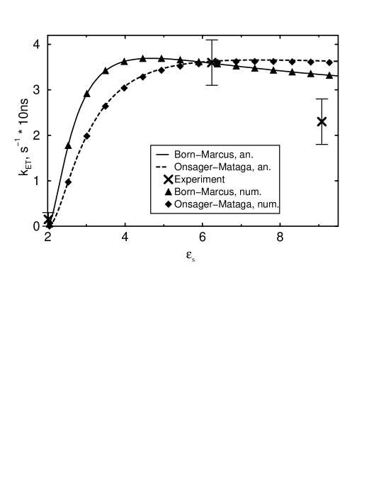
Figure 4.9: The transfer rate $k_{\rm ET}$ versus static dielectric constant. The energy of bridging and acceptor states scales in accordance with Born expression (4.8) (triangles and solid line), Onsager expression (4.9) (diamonds and dashed line). Coherent couplings and dissipation scales in accordance with Mataga’s expression (4.23) (diamonds and dashed line), Georgievskii-Marcus expression (4.24) (triangles and solid line). Symbols represent numerical solution of system of Eqs. (4.20)-(4.21). Lines represents analytical result Eq. (4.32). Solid crosses with error bars correspond to experimental values [140].

For the application of the results to various solvents and comparison with experiment one should use the scaling for energy, coherent coupling, and dissipation as discussed above. The combinations of the energy scaling mentioned in subsection 4.2.1 and relaxation intensities scalings mentioned in subsection 4.2.4 are represented in Fig. 4.9. An increase in the static dielectric constant $\epsilon_{\rm s}$ from $2$ to $4$ leads to an increase of the transfer rate, no matter which scaling is used. Further increase of $\epsilon_{\rm s}$ induces saturation for the Onsager-Mataga scaling and even a small decrease of the transfer rate for the Born-Marcus scaling. In all those cases the solvent is approximated as the continuous medium. Thus, the transfer rate depends on the interplay of the two mechanisms. Within the used approximations an increase in the solvent polarizability and, hence, of its dielectric constant lowers the energy of the bridging and acceptor states and increases the system-bath interaction and, hence, the relaxation coefficients. It induces a smooth rise of the transfer rate in the whole interval of $\epsilon_{\rm s}$ for the Onsager-Mataga scaling. On the other hand the large values of dielectric constant lead to essentially different polarisational states of the environment for the aggregate states with different dipole moment. The difference of the environmental polarizations reduces the values of the coherent couplings, see Eq. (4.25). This effect is reflected for the Born-Marcus scaling in the small decrease of $k_{\rm ET}$ for large values of $\epsilon_{\rm s}$. The values for the transfer rate, obtained with this scaling come closer to the experimental value $k_{\rm ET}(\epsilon_{\rm s}^{\rm CH_{2}Cl_{2}})$. This gives a hint that the model of individual cavities for each molecular block is closer to the reality than the model with a single cavity for the whole supermolecule.

Below we consider Born scaling Eq. (4.8) for the system energies and Marcus scaling Eq. (4.24) for the dissipation parameter to compare the calculated transfer rates with the measured ones. For the solvents CYCLO, MTHF, and ${\rm CH_{2}Cl_{2}}$ one obtains the following relative energies of the bridging level $E_{21}=1.77~{}{\rm eV}$, $1.36~{}{\rm eV}$, and $1.30~{}{\rm eV}$, respectively, i.e., a decrease in the energy of the bridging state.

The calculated transfer rate coincides with the experimental value [140] for ${\rm H_{2}P-}$ ${\rm ZnP-}$ ${\rm Q}$ in CYCLO, see table 4.2. For ${\rm CH_{2}Cl_{2}}$ the numerical transfer rate diverges from the experimentally determined one. The calculated numerical value is found to be approximately thirty percent faster. The following reasons could be responsible for this difference: (i) absence of vibrionic substructure of the electronic states in the present model; (ii) incorrect dependence of system state energies on the solvent properties; (iii) appearing of additional transfer channels not mentioned in the scheme shown in Fig. 4.2. Each of these possibilities requires some comments.

ad (i): The incorporation of the vibrational substructure will result in a complication of the model with parameters such as the mass of each vibrational mode [12, 180]. It will also give a more complicated transfer rate dependence on the energy of the electronic states and dielectric constant. In the model with vibrational substructure the interplay between the difference of the energies of each pair of electronic states and corresponding reorganization energy determines if the pair belongs to the normal, activationless, or inverted region according to Marcus [155]. In contrast to the present consideration the model with vibrational substructure should yield the maximal transfer rate for nonequal energies of electronic state, namely for the activationless case: the energy difference equals to the reorganization energy. For a detailed comparison of TB model and the model with vibrational substructure see the next section.

ad (ii): In particular such solvent effect as solvation shell, see for example Ref. [184], do need a molecular dynamics simulation. The total influence of solvent is, probably, reflected in solvent-induced energy shift between the spectroscopically observable states without charge separation $E_{\rm D^{*}BA}$ and $E_{\rm DB^{*}A}$ [140] which is neglected in our consideration.

ad (iii): Some states of our three-site system have not been included in the model schematically presented in Fig.  4.2. Using the solvent with strong dielectric constant can bring high-lying states closer to the ones involved in the transfer. The state which might play a role is $\left|{\rm D^{-}B^{+}A}\right>$ because of its larger dipole moment. So it is strongly influenced by the solvent. The state $\left|{\rm DBA^{*}}\right>$ which has such a high energy that one can excite it only with ultraviolet radiation, most probably, does not play a role in the discussed transfer.

4.5.3 Comparison with the steady-state solution

In the work of Davis et al. [10] the vibrational substructure of the electronic states is also not taken into account, the relaxation is incorporated phenomenologically. We use a similar approach in the present consideration derived within a Redfield-like theory. Also we consider the relevant processes of dephasing and depopulation between each pair of levels. In contrast Davis et al. apply relaxation only to selected levels. In their paper dephasing $\gamma$ occurs between excited levels, see Eq. (7) in Ref. [10], while depopulation $k$ takes place only for the transition from acceptor to ground state. The advantage of the approach of Davis et al. is the possibility to investigate the transfer rate dependence for more than one bridge state. This was not the goal of the present work but it can be extended into this direction. We are interested in the ET in a concrete molecular complex with realistic parameter values and realistic possibilities to modify those parameter. Our results as well as the results of Davis show that ET can occur as coherent (with the superexchange mechanism) or dissipative process (with the sequential mechanism). We have considered various ways of switching between these two mechanisms including the one suggested by Davis et al., i. e., the change of the relaxation intensities meaning change of the solvent. The numerical steady state method used by Davis et al. is an attractive one due to its simplicity, but unlike our method it is not able to give information about the time evolution of the system. On the other hand the method of Davis et al. does not allow to calculate the most widespread stationary characteristics that clarify the presence of ET process, namely the fluorescence of the donor and its quenching. We suppose this can be included into the approach by Davis et al. by introducing the depopulation coefficient describing the transfer from donor to ground state.

4.6 Vibronic model

In the model with vibrational substructure (VSS) the influence of the interaction with an environment onto ET and other dynamical processes is also described by the common Hamiltonial of the form Eq. (2.1).

The bath again is modeled by a distribution of HOs and characterized by its spectral density $J(\omega)$. Starting with a DM of the full system, the RDM of the relevant (sub)system is obtained by tracing out the bath degrees of freedom [73]. While doing so a second-order perturbation expansion in the system-bath coupling and the Markov approximation have been applied [73]. So one arrives at the RDMEM of the already discussed structure.

 

Figure 4.10: Electronic potentials and parameters of the vibronic model. The donor surface $\left.{\rm H_{2}P}^{*}-{\rm ZnP}-{\rm Q}\right.$ is given by the solid line, the bridge $\left.{\rm H_{2}P}^{+}-{\rm ZnP}^{-}-{\rm Q}\right.$ by the dashed line, and the acceptor $\left.{\rm H_{2}P}^{+}-{\rm ZnP}-{\rm Q^{-}}\right.$ by the dotted line.

The bridge ET system ${\rm H_{2}P}-{\rm ZnP}-{\rm Q}$ is modeled by three diabatic electronic potentials, corresponding to the states $\left|1\right>=\left|{\rm D}^{*}{\rm B}{\rm A}\right>$, $\left|2\right>=\left|{\rm D}^{+}{\rm B}^{-}{\rm A}\right>$, and $\left|3\right>=\left|{\rm D}^{+}{\rm B}{\rm A^{-}}\right>$ (see Fig. 4.10). Each of these electronic potentials has a vibrational substructure. The vibrational frequency is assumed to be 1500 cm^-1 as a typical frequency within carbon structures. The potentials are displaced along a common reaction coordinate which represents the solvent polarization [155]. Following the reasoning of Marcus [155] the free energy differences $\Delta G_{\mu\nu}$ corresponding to the ET from molecular block $\nu$ to $\mu$ ($\nu=1$, $\mu=2,3$) are estimated to be [183, 140]

$$\Delta G_{mn}=E_{\mu}^{\rm ox}-E_{\nu}^{\rm red}-E^{\rm ex}-\frac{e^{2}}{4\pi\epsilon_{0}\epsilon_{\rm s}}\frac{1}{r_{\mu\nu}}+\Delta G_{\mu\nu}(\epsilon_{\rm s})$$ (4.37)

with the term $\Delta G_{\mu\nu}(\epsilon_{\rm s})$ correcting for the fact that the redox energies $E^{\rm ox}_{\mu}$ and $E^{\rm red}_{\nu}$ are measured in the reference solvent with dielectric constant $\epsilon_{\rm s}^{\rm ref}$:

$$\Delta G_{mn}(\epsilon_{\rm s})=\frac{e^{2}}{4\pi\epsilon_{0}}\left(\frac{1}{2r_{\mu}}+\frac{1}{2r_{\nu}}\right)\left(\frac{1}{\epsilon_{\rm s}}-\frac{1}{\epsilon_{\rm s}^{\rm ref}}\right).$$ (4.38)

The excitation energy of the donor ${\rm H_{2}P}\to{\rm H_{2}P}^{*}$ is denoted by $E^{\rm ex}$. $r_{\nu}$ denotes the radius of either donor (1), bridge (2), or acceptor (3) and $r_{\mu\nu}$ the distance between two of them as presented in section 4.3.

Also sketched in Fig. 4.10 are the reorganization energies $\lambda_{\mu\nu}=\lambda_{\mu\nu}^{\rm i}+\lambda_{\mu\nu}^{\rm s}$. These consist of the internal reorganization energy $\lambda_{\mu\nu}^{\rm i}$, which is estimated to be 0.3 eV [140], and the solvent reorganization energy [155]

$$\lambda_{\mu\nu}^{\rm s}=\frac{e^{2}}{4\pi\epsilon_{0}}\left(\frac{1}{2r_{\mu}}+\frac{1}{2r_{\nu}}-\frac{1}{r_{\mu\nu}}\right)\left(\frac{1}{\epsilon_{\infty}}-\frac{1}{\epsilon_{\rm s}}\right)~{}.$$ (4.39)

Further parameters are the electronic couplings between the potentials. They are the same as described in section 4.3. The damping is described by the spectral density $J(\omega)$ of the bath. This is only needed at the frequency of the vibrational transition and is determined $J(\omega_{\rm vib})/\omega_{\rm vib}=0.372$ by fitting the ET rate for the solvent methyltetrahydrofuran (MTHF). In the vibronic model the spectral density is taken as a constant with respect to $\epsilon_{\rm s}$.

Next the calculation of the dynamics is sketched. Starting from the Liouville equation, performing the abovementioned approximations the equation of motion for the RDM $\rho_{\cal{M}\cal{N}}$ can be obtained [136, 137]

$$\frac{\partial}{\partial t}\rho_{\cal{M}\cal{N}}=\frac{i}{\hbar}(E_{\cal{M}}-E_{\cal{N}})\rho_{\cal{M}\cal{N}}-i\sum_{\cal{K}}\{v_{\cal{N}\cal{K}}\rho_{\cal{M}\cal{K}}-v_{\cal{K}\cal{M}}\rho_{\cal{K}\cal{N}}\}+R_{\cal{M}\cal{N}}~{}.$$ (4.40)

The index $\cal{M}$ combines the electronic quantum number $\mu$ and the vibrational quantum number ${M}$ of the diabatic levels $E_{\cal{M}}$. $v_{\cal{M}\cal{N}}=V_{\mu\nu}F_{\rm FC}(\mu,{M},\nu,{N})$ comprises Franck-Condon factors $F_{\rm FC}$ and the electronic matrix elements $V_{\mu\nu}$. The third term $R_{\cal{M}\cal{N}}$ describes the interaction between the relevant system and the heat bath. In principle one can eliminate the coherent terms containing $v_{\cal{K}\cal{M}}$ diagonalising the Hamiltonian of the isolated system. In such approach one couples the environment transitions to the transitions between the eigenstates of the system. This is adiabatic approach, used in e.g. [145]. It is rather expensive numerically. We do not apply it here, so we use the diabatic approach. There are still a discussion in the literature wether the diabatic method is able to provide precise results [185]. Nevertheless one uses the diabatic approach rather often [136, 137] because it is less expensive numerically [186].

Equation (4.40) is solved numerically with the initial condition that only the donor state is occupied in the beginning. The population of the acceptor state

$$P_{3}(t)=\sum\limits_{M}\rho_{3M3M}(t)$$ (4.41)

and the ET rate given by Eq. (4.28) are calculated by tracing out the vibrational modes.

4.7 Comparison of models with and without vibrations

Here we compare the following models: (i) the model where only electronic states without vibrational substructure are taken into account (see Fig. 4.5) and relaxation processes take place between the electronic states and (ii) the model where the relaxation takes place between vibrational states within one electronic state potential surface introduced in the previous section.

In this section the energies of the electronic states $E_{m}$ of model without vibrational substructure are chosen to be the ground states of the harmonic potentials of the vibronic model shown in Fig. 4.10. So they vary with the dielectric constant. The electronic couplings are chosen to scale as Eq. (4.25). Note, that in the model with vibrational substructure it corresponds to the scaling provided by the Franck-Condon overlap elements between the vibrational ground states of each pair of electronic surfaces

$$v_{\cal{M}\cal{N}}=V_{\mu\nu}F_{\rm FC}(\mu,0,\nu,0)=V_{\mu\nu}\exp{\frac{-|\lambda_{\mu\nu}|}{2\hbar\omega_{\rm vib}}}~{}.$$ (4.42)

Here we have used the expression for the Franck-Condon factor for the parabolas with equal effective mass $m$, and equal curvature $F_{\rm FC}(\mu,0,\nu,0)=\exp{(-\frac{m\omega_{\rm vib}}{2\hbar}\Delta q_{\mu\nu}^{2})}$ and definition of reorganization energy $\lambda_{\mu\nu}=m\omega_{\rm vib}^{2}\Delta q_{\mu\nu}^{2}$. $q_{\mu\nu}$ stands for the difference of the reaction coordinate equilibrium points of these parabolas. In the vibronic model not only the free energy differences $\Delta G$ but also the reorganization energies $\lambda$ scale with the dielectric constant $\epsilon_{\rm s}$. Due to this scaling of $\lambda$ the system-bath interaction is scaled with the dielectric constant $\epsilon_{\rm s}$. In the high temperature limit the reorganization energy is given by [157]

$$\lambda=\hbar\int_{0}^{\infty}d\omega\frac{J(\omega)}{\omega}~{}.$$ (4.43)

This relation can be taken as motivation to scale the TB spectral density with $\epsilon_{\rm s}$ like the reorganization energies $\lambda$ in the model with vibrational substructure as discussed in the subsection 4.2.4. In the present calculations $\Gamma_{21}=\Gamma_{23}=\Gamma$ is assumed. The absolute value of the damping rate $\Gamma$ between the electronic states (see Fig. 4.5) in this section is determined by fitting the ET rate for the solvent MTHF to be $\Gamma=2.9\times{}10^{11}$ s^-1. It differs from the value given in section 4.5 because the different energies of states have been used here.

 

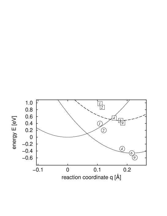
Figure 4.11: Variation of the potential minima for different solvents. Squares denote the bridge minima, circles the acceptor minima. The numbers correspond to the ordinal numbers in Table 4.3. The potentials are shown for solvent 6 (MTHF).

The advantage of the TB model in comparison to the model with vibrational substructure is the possibility to determine the transfer rate $k_{\rm ET}$ and the final population of the acceptor state either numerically or analytically. For all situations described in this paper the differences between analytic and numerical results without the extra assumptions are negligible as shown in section 4.5.

In Fig. 4.11 it is shown how the minima of the potential curves change with varying the solvent due to the changes in Eqs. (4.37) to (4.39).

Table 4.3: Parameters and obtained transfer rates for different solvents. The references behind the names of the solvents cite the sources of $\epsilon_{\rm s}$ and $\epsilon_{\infty}$. $\Gamma$ denotes the damping rate in the TB model. The ET rate for the solvent MTHF has been used to fix the damping parameter of the models. The reaction rates $k_{\rm ET}^{\rm el}$ were obtained using Eq. (4.32) within the TB model and the reaction rates $k_{\rm ET}^{\rm vib}$ within the vibronic model.

solvent	$\epsilon_{\rm s}$	$\epsilon_{\infty}$	$\Delta G_{21}$	$\Delta G_{31}$	$\lambda_{21}^{\rm s}$	$\lambda_{31}^{\rm s}$	$\Gamma$	$k_{\rm ET}^{\rm el}$	$k_{\rm ET}^{\rm vib}$
			[eV]	[eV]	[eV]	[eV]	[$10^{11}$ s-1]	[$10^{8}$ s-1]	[$10^{8}$ s-1]
1. CYCLO [140]	2.02	2.00	0.976	0.393	0.007	0.012	0.042	0.181	0.7
2. toluene [187]	2.38	2.24	0.867	0.202	0.039	0.069	0.227	1.04	0.8
3. anisole [188]	4.33	2.29	0.590	-0.281	0.300	0.524	1.751	4.24	2.30
4. dibromoethane [188]	4.78	2.37	0.558	-0.336	0.312	0.544	1.817	4.63	2.45
5. chlorobenzene [187]	5.29	1.93	0.529	-0.388	0.481	0.839	2.804	3.21	3.63
6. MTHF [140]	6.24	2.00	0.486	-0.462	0.497	0.868	2.900	3.59	3.58
7. methyl acetate [187]	6.68	1.85	0.471	-0.489	0.571	0.996	3.328	2.96	4.15
8. trichloroethane [188]	7.25	2.06	0.454	-0.512	0.508	0.887	2.960	3.98	3.50
9. dichloromethane [140]	9.08	2.03	0.413	-0.590	0.559	0.977	3.264	4.00	3.80

The solvents are listed in Table 4.3 together with their parameters and the results for the ET rates in both models. For larger $\epsilon_{\rm s}$ the coordinates of the potential minima of bridge and acceptor increase while their energies decrease with respect to the energy of the donor. The energy difference between donor and bridge decreases with increasing $\epsilon_{\rm s}$. This makes a charge transfer more probable. For small $\epsilon_{\rm s}$ the acceptor state is higher in energy than the donor state; nevertheless there is a small ET rate due to coherent mixing. For fixed $\epsilon_{\infty}$ the ET rate is plotted as a function of the dielectric constant $\epsilon_{\rm s}$ in Fig. 4.12. The ET rate in the vibronic model increases strongly for small values of $\epsilon_{\rm s}$ while the increase is very small for $\epsilon_{\rm s}$ in the range between 5 and 8. The increase for small values of $\epsilon_{\rm s}$ is due to the fact that with increasing $\epsilon_{\rm s}$ the minimum of the acceptor potential moves from the position higher than the minimum of the donor level to the position lower than the donor level. So the transfer becomes energy favorable. This can also be seen when looking at the results for the TB model without scaling the electronic coupling with the Franck-Condon factor. In this case the ET rate increases almost linearly with increasing $\epsilon_{\rm s}$. The effect missing in this model is the overlap between the vibrational states. If one corrects the electronic coupling in the TB model by the Franck-Condon factor of the vibrational ground states as described in Eq. (4.42), good agreement is observed between the vibronic and the TB model.

 

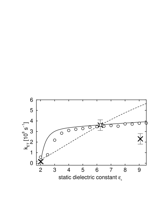
Figure 4.12: Transfer rate as a function of the dielectric constant $\epsilon_{\rm s}$ for both models together with experimental results [140]. The rates for the vibronic model are given by the circles. The dashed line shows the rate for the TB model with electronic couplings $V_{mn}$ as in the vibronic model. The solid line represents the rate for the TB model with $v_{mn}$ scaled as given in Eq. (4.42).

The ET rate for the vibronic model shows some oscillations as a function of $\epsilon_{\rm s}$. This is due to the small density of vibrational levels in this model with one reaction coordinate. All three electronic potential curves are harmonic and have the same frequency. So there are small maxima in the rate when two vibrational levels are in resonance and minima when they are far off resonance. Models with more reaction coordinates do not have this problem nor does the simple TB model. If these artificial oscillations would be absent, the agreement between the results for the TB and the vibronic model would be even better, because the rate for the vibronic model happens to have a maximum just at the reference point $\epsilon_{\rm s}=6.24$ which we have chosen to fix the spectral density, i. e. for MTHF.

The comparison of the two models has been made assuming that the scaling of energies as a function of the dielectric function is correct in the Marcus theory. There have been a lot of changes to Marcus theory proposed in the last years. Marcus theory assumes excess charges within cavities surrounded by a polarizable medium and there one only takes the leading order into account. Higher order terms are included in the so called reaction field theory (see for example [175]). But to compare different solvation models is out of the range of the present investigation. Some more details on this issue for the TB model are already given in section 4.2. Here we just want to note that the effect of scaling the system-bath interaction with $\epsilon_{\rm s}$, as assumed in the present work for the TB model, has no big effect on the ET rates.

4.8 Summary

We have performed a study of the ET in the supermolecular complex ${\rm H_{2}P}-{\rm ZnP}-{\rm Q}$ within the TB model treated with the DM formalism. The determined analytical and numerical transfer rates are in a reasonable agreement with the experimental data. The superexchange mechanism of ET dominates over the sequential one. We have investigated the stability of the model varying one parameter at a time. The qualitative character of the transfer is stable with respect to a local change of system parameters. It is determined that the change of the dominating transfer mechanisms can be induced by lowering the bridge state energy. The physical reasons of system parameters scaling as well as the relation of the theory presented here to other theoretical approaches to ET have been discussed.

The validity of the TB model and its applicability to ${\rm H_{2}P}-{\rm ZnP}-{\rm Q}$ is confirmed because one gets good agreement for the ET rates of the models with and without vibrational substructure, i. e. the vibronic and the TB model, if one scales the electronic coupling with the Franck-Condon overlap matrix elements between the vibrational ground states. The advantage of the model with electronic relaxation only is the possibility to derive analytic expressions for the ET rate and the final population of the acceptor state. But of course for a more realistic description of the ET process in such complicated systems as discussed here, more than one reaction coordinate should be taken into account.

The calculations performed in the framework of the present formalism can be extended in the following directions: (i) Considerations beyond the kinetic limit. The solvent dynamics has to be included into the model as well as, probably, non-Markovian RDM equations. (ii) Enlargement of the number of molecular blocks in the complex. (iii) Initial excitation of states with rather high energy should open additional transfer channels.

Chapter 5 Mixture of Solvents

In this chapter we apply the RDM method which was described in chapter 2 to another experimental system i. e. porphyrin triad complexes. This method provides a quantitative description of time-resolved and steady-state properties such as fluorescence quenching of the porphyrins. It will be shown that our calculations do agree with already performed experiments.

We start this chapter with a brief review of an important role of the supramolecular porphyrin array in electronic energy transfer, charge transfer, and photoinduced structural changes in biological systems since such processes constitute the basis for the design of molecular devices of applicative interest and for the understanding of the most important photobiological processes. First, in section 5.1 we introduce the chemical structure of the self-assembled porphyrin triad ${\rm ZnPD-H_{2}P}$. Next, in section 5.2 we qualitatively describe the photophysics of the porphyrin triad in different solvents with various dielectric constants. In section 5.3 the parameters of the RDM formalism are discussed and determined for both the porphyrin complexes and the quantitative description of the fluorescence quenching. The explanation of the fluorescence quenching is done in subsection 5.4.1. The analysis of our calculations and the experimental results performed in subsection 5.4.2 yield valuable information about the reaction mechanisms. Finally, in section 5.5 we summarize the achievements of this chapter. Some generalizations are transferred to the Appendix B and require more detailed consideration in the future.

5.1 Self-assembled triad of porphyrins

Because of their widespread occurrence in photosynthetic reaction centres and other electron-transfer systems supramolecular porphyrin arrays have played a leading role in the study of energy and charge transfer processes in biological systems [189, 190, 191, 192, 193, 194] or to gain insight into the principal possibilities of molecular electronics[195]. Among supramolecular porphyrin arrays three-component covalently-linked donor-acceptor systems [196, 197] have attracted a lot of interest, especially, in the context of photochemical molecular devices [198, 199]. Besides, it is possible to form donor-acceptor systems using both covalent bond and non-covalent binding self-assembling based on coordination interactions of metallo-porphyrins with appropriate extra ligands[200, 201, 202]. These systems are formed from chemical dimer of Zn-octaethylporphyrin with a phynyl spacer (ZnPD) and dipyridyl-diphenylporphyrin with nitrogens in meta-positions of pyridil rings (${\rm H_{2}P}$) via two-fold coordination of two central Zn ions of the dimer with pyridil rings of the extra-ligand. The chemical structure of a self-assembled porphyrin triad is represented in Fig. 5.1.

 

 

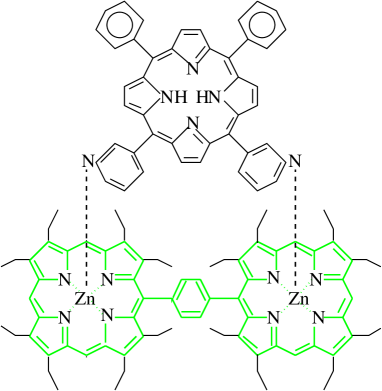
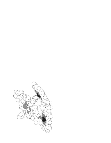
Figure 5.1: Schematic presentation of ${\rm ZnPD-H_{2}P}$.

It was experimentally found in these systems [201] that the population of the excited state of ${\rm H_{2}P}$ is dependent on the solvent dielectric constant as well as on temperature. This is attributed to a close lying charge separated state which exchanges rapidly with the exited state of ${\rm H_{2}P}$.

5.2 Photophysics of a porphyrin triad

As determined by fluorescence spectroscopic measurements [201], where one excites ${\rm ZnPD}$, the triadic aggregate in non-polar solvents (toluene, methylcyclohexane) demonstrates fluorescence quenching for ${\rm ZnPD}$ and quite intensive fluorescence for ${\rm H_{2}P}$. It is reasonable to assume that energy transfer processes may be involved in this quenching. The fluorescence ${\rm ZnPD-H_{2}P^{*}\to ZnPD-H_{2}P}$ (characterized by the fluorescence time $\tau_{\rm F}=7.7$ ns) is less intensive with respect to that for pure ${\rm H_{2}P^{*}\to H_{2}P}$ ($\tau_{\rm F}=9.3$ ns) at the same conditions [201]. The quenching of ${\rm H_{2}P}$ fluorescence increases with the polarity of the solvent. To check whether this is the case an experiment has been performed [201]. In this experiment the triadic complexes were formed in a solution of pure toluene (low dielectric constant) and then in an admixture of acetone (up to 20%) added to toluene (relatively high dielectric constant). In the first case the aggregate shows fluorescence with the mean band maximum of $716$ nm which is attributed to ${\rm H_{2}P}$ and fluorescence excitation spectra clearly demonstrate the presence of an energy transfer. While in the second case ${\rm H_{2}P}$ shows noticable fluorescence quenching. Thus the excitation is lost without radiation and ET must take place.

 

Figure 5.2: Scheme of the photoinduced processes.

The physics of this reaction is qualitatively shown in Fig. 5.2, where D and A represent the electron donor ${\rm ZnPD}$ and the electron acceptor ${\rm H_{2}P}$, respectively. Note that here D and A denote other compounds than in chapter 4 while the symbols of plus, minus, and star are defined in the same way as in section 4.2. Light excitation of ${\rm ZnPD}$ to its singlet state $\left|1\right\rangle$ is followed by weak dissipative energy transfer to the exited state $\left|3\right\rangle$ (process a). Inaddition to this process, an ET (process b) takes place, leading to the charge-separated state $\left|2\right\rangle$. The evolution of the population of this state $\left|2\right\rangle$ is distributed between charge recombination (does not enter into the scheme) and further weak coherent and dissipative charge transfer (process c) to give the state $\left|3\right\rangle$. Because the decay of the charge-separated state occurs quite slowly for porphyrin-type systems [203], we do not consider this process and do not include it in Fig. 5.2. The energy of state $\left|2\right\rangle$ depends on the dielectric constant of the solvent.

5.3 Density matrix model parameters

The RDM model is able to describe coherent dynamics, dissipative dynamics, and thermally activated processes, thus the RDM formalism can be used for a quantitative explanation of the reaction which was described in subsection 5.2. We apply the system of equations (4.20)-(4.21) to describe the processes in the porphyrin triad.

To calculate the population of the excited states physically reasonable values of the model parameters, such as coherent and dissipative couplings and energy of states have been chosen. The physical behavior of the system is determined in leading order by the energies. remains rather stable in respect to change of other parameters. Nevertheless it is reasonable to give some physical foundation in which region the parameters values should lie.

In accordance with the consideration given in section 4.7 the parameters for the model with only electronic states can be extracted using some properties of the appropriate model with vibrational substructure. In such model one describes the porphyrin triad with the relevant potential energy surfaces in the space of a single reaction coordinate which reflect the extent of the solvent polarization induced by the field of the triad. In order to allow the analysis of absorption and emission spectra one should add to the model a ground state potential $\left|0\right>$. For the neutral excited states $\left|1\right>$ and $\left|3\right>$ the difference in absorption and emission spectra of the transition ground-excited determines the shift $q_{i0}$ of the equilibrium point of the excited state $\left|i\right>$ in respect to the equilibrium point of the ground state $\left|0\right>$. The shift of the equilibrium point of the state $\left|2\right>$ with charge separation can be calculated using the reorganization energy Eq. (4.39).

We assume that the sign of the shift for the state $\left|3\right>$ should be negative in respect to the signs of the shifts of $\left|1\right>$ and $\left|2\right>$. To check whether it is really so one should analyse the dependence of $\left|1\right>\to\left|3\right>$ transition rate on the solvent polarity. Supposing that the vibrational excitations again do not play a role and in accordance with the explanation after the Eq. (4.42) the coherent couplings can be expressed as $v_{12}=V_{12}\exp{\left[-{(2\hbar\omega_{\rm vib})^{-1}}{(q_{20}-q_{10})^{2}}\right]}$, $v_{23}=V_{23}\exp{\left[-{(2\hbar\omega_{\rm vib})^{-1}}{(q_{20}-q_{30})^{2}}\right]}$ etc.. Therefore the relation of the coherent couplings reads

$${v_{12}}/{v_{23}}={V_{12}}/{V_{23}}\exp\left\{-{(2\hbar\omega_{\rm vib})^{-1}}[q_{10}^{2}-q_{30}^{2}-2q_{20}(q_{10}-q_{30})]\right\}.$$

For $q_{10}\sim-q_{30}$ and $q_{20}\gg-q_{30}$ the exponential reads $\exp\left[-{(2\hbar\omega_{\rm vib})^{-1}}\right.$ $\left.{4q_{20}q_{10}}\right]$. This is an exponential of a positive argument so the $v_{12}$ should be at least $e$ times larger as $v_{23}$.

Table 5.1: Coherent and dissipative couplings between the electronic states.

Coupling	Value, meV	Physical Process	Comment
$v_{12}$	60	electron transfer $D^{*}A\to D^{+}A^{-}$	induced by the wavefunction overlap
$v_{32}$	3	hole transfer $DA^{*}\to D^{+}A^{-}$	weakened by the screening field of the electron from the LUMO of the acceptor
$v_{13}$	12	energy transfer $D^{*}A\to DA^{*}$	induced by the dipole-dipole interaction of the excited states $v_{13}\sim p_{\mathrm{D^{*}A}}p_{\mathrm{DA^{*}}}/{r_{\mathrm{DA}}}^{3}$
$\Gamma_{12}$	0.41	loss of coherence for $D^{*}A\to D^{+}A^{-}$	interaction of the transition dipole moment with environmental dipoles
$\Gamma_{32}$	2.50	loss of coherence for $DA^{*}\to D^{+}A^{-}$	induced by the interaction with the environment
$\Gamma_{13}$	0.37	loss of coherence for $D^{*}A\to DA^{*}$	estimated by taking into account other dissipation $\gamma_{ij}=\sum\limits_{k}(d_{ik}+d_{kj})$

The electronic matrix elements $V_{\mu\nu}$ should also have a difference because the $\left|3\right>\to\left|2\right>$ process imply the ET from one inner orbital ${\rm HOMO_{D}}$ to another inner orbital ${\rm HOMO_{A}}$. So for the first attempt we take $v_{12}=0.06~{}{\rm eV}$ as typical value of the coupling between porphyrins (same as the coupling $\left<{\rm H_{2}P^{*}-ZnP-Q}|H|{\rm F_{2}P^{+}-ZnP^{-}-Q}\right>$ for zinc-porphyrin-quinone complex in chapter 4 with the precision up to the first significant figure) and $v_{32}=0.003~{}{\rm eV}$ is taken to be 20 times smaller.

The range of reasonable values of relaxation constants $\Gamma_{\mu\nu}$ can be estimated using Eq. (4.43) and reorganisanization energies from the model with vibrations. The values of the couplings are represented in Tab. 5.1. The precise determination of the parameters needs a special investigation within quantum chemical calculations. This is the next step in the theoretical description of this porphyrin triad. The quantum chemical calculation of the couplings should be done in the future.

 

Figure 5.3: Energy difference between states $\left|2\right>$ and $\left|3\right>$

The excited state energies $E_{\rm D^{*}A}=2.10$ eV and $E_{\rm DA^{*}}=1.91$ eV are found spectroscopically [140]. The energy of the state $\left|2\right>$ needs more attention. It depends on the solvent and can be calculated in any solvent with the help of Weller’s formula [204]:

$$E_{{\rm D^{+}A^{-}}}({\epsilon})=E_{\rm{D^{+}A^{-}}}({\epsilon_{\rm{t}}})+\left(\frac{1}{{\epsilon}}-\frac{1}{{\epsilon_{\mathrm{t}}}}\right)\times\frac{e^{2}}{4\pi\epsilon_{0}}\left(\frac{1}{2r_{\rm D}}+\frac{1}{2r_{\rm A}}-\frac{1}{r_{\rm DA}}\right),$$ (5.1)

where $\epsilon$ denotes the solvent static dielectric constant, $r_{\rm D}=r_{\rm A}=5.5~{}{\rm\AA}$ are the donor and acceptor radius, respectively, $r_{\rm DA}=8.8~{}{\rm\AA}$ is the distance between them. In our case the solvent consists of the main compound toluene with a dielectric constant ${\epsilon_{\mathrm{t}}}$ and a small concentration $c$ of the additional compound acetone with a dielectric constant ${\epsilon_{\mathrm{a}}}$. In accordance with [205] the effective dielectric constant of the mixture reads

$$\epsilon=\epsilon_{\rm t}+c\frac{3(\epsilon_{\rm a}-\epsilon_{\rm t})\epsilon_{\rm t}}{\epsilon_{\rm a}+2\epsilon_{\rm t}}.$$ (5.2)

The change of $\epsilon$ induces an energy shift of the state $\left|2\right>$. We present the energy difference $\Delta E=E_{3}-E_{2}$ between states $\left|3\right>$ and $\left|2\right>$ as a function of $c$ in Fig. 5.3. The values $E_{\mathrm{D^{+}A^{-}}}=1.90$ eV, ${\epsilon_{\mathrm{t}}=2.38}$ for the pure toluene solution and ${\epsilon_{\mathrm{a}}=10}$ for the acetone were defined in [201].

5.4 Physical processes

5.4.1 Fluorescence quenching: simulations and experiment

In the porphyrin triad the competition between charge transfer and energy transfer (process a and b in Fig. 5.2, respectively) cause a rather complex dynamics. Mathematically it is easy to calculate the system state at the infinite time $t=\infty$. For our real system the electron transfer time $\tau_{\rm ET}$ is much shorter than the time of fluorescence $\tau_{\rm F}$. Thus we approximate $t=\infty$ with some time moment when the ET has finished and the fluorescence has not occured yet. On this time $\tau_{\rm ET}<t<\tau_{\rm F}$ the system reaches the quasi thermal equilibrium between the excited state $\left|3\right\rangle$ and the close lying charge separated state $\left|2\right\rangle$.

 

 

Figure 5.4: Solvent induced fluorescence quenching, $T=293~{}{\rm K}$ (left); freezing induced fluorescence quenching, $c_{\rm a}=7\%$ (right).

We have calculated the equilibrium population of the state $\left|3\right\rangle$ numerically with the RDM-method. This population corresponds to the presence of the fluorescence into the ground state. We denote the population of this state with $P_{\rm DA^{*}}=\rho_{33}$.

It has been found that $\rho_{33}(\infty)$ decreases in two cases: (i) lowering of the energy $E_{\rm D^{+}A^{-}}$ induced by increase of aceton concentration, see Fig. 5.4 (left) and (ii) lowering of the temperature, see Fig. 5.4 (right) This decrease corresponds to the experimentally observed fluorescence quenching [201].

5.4.2 Reaction mechanisms

The variation of the acetone admixture concentration and temperature changes the fluorescence intensity $\rho_{33}$ as well as a character of the excited states dynamics. Our simulations display that the time dependence of the population $\rho_{33}$ (Fig. 5.5) as well as its temperature dependence (Fig. 5.6) at low acetone concentration qualitatively differs from the behavior at high acetone concentration. This is the most important result of the RDM-calculations. It demonstrates the qualitatively different reaction mechanisms under various experimental conditions.

 

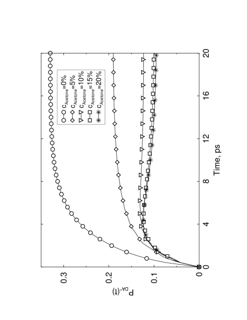
Figure 5.5: Influence of concentration on the reaction mechanism, $T=293~{}{\rm K}$, at low $c_{\rm a}$ the reaction passes in one step (circles and diamonds), high $c_{\rm a}$ induces the two-step reaction mechanism (triangles, squares, and stars).

A low concentration of acetone induces a low energy detuning between the states $\left|2\right\rangle$ and $\left|3\right\rangle$. In this case (see Fig. 5.6 for small $c_{\rm a}$ ), $\rho_{33}$ starts to increase with time due to energy transfer (process a) and then does not change as $\left|3\right\rangle$ reaches the quasi-thermal equilibrium. Thus the equilibrium population $\rho_{33}(\infty)$ is reached in one-step and a reaction rate $k$ can be found with an one-exponential fit Eq. (4.28).

As shown in Fig. 5.3 in the case of high aceton concentration the energy detuning between states $\left|2\right>$ and $\left|3\right>$ becomes larger and in addition to the energy transfer (process a), the hole transfer (process c) takes place, thus the equilibrium population $\rho_{33}$ is reached in two steps. At first, the energy transfer creates a time-dependent maximum of the population of $\left|3\right\rangle$ (see Fig. 5.6 for large $c_{\rm a}$) and then hole transfer $\left|3\right\rangle$ $\rightarrow$ $\left|2\right\rangle$ slowly induces depopulation of $\left|3\right\rangle$ down to the equilibrium population. The reaction occurs with the help of a sequential transfer, which is described by two rates (increase and decrease) and the one-exponential fit for $k$ cannot be used in this case.

 

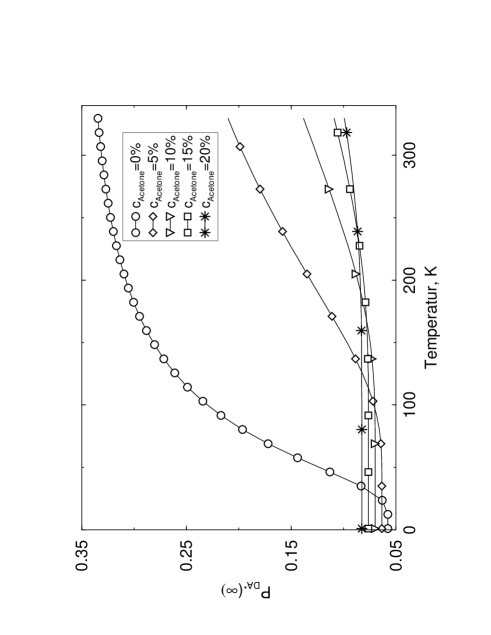
Figure 5.6: Thermally activated mechanism, the population remains constant until energy difference is lower than the thermal energy.

The temperature dependence of $\rho_{33}(\infty)$ (Fig. 5.7) also reflects the change of the reaction mechanism which depends on the acetone concentration and temperature. For a low acetone concentration the equilibrium population $\rho_{33}(\infty)$ increases with temperature because $\Delta E$ between states $\left|3\right>$ and $\left|2\right>$ is lower than the thermal energy. This case corresponds to a one-step reaction.

In the case of a high acetone concentration $\Delta E$ becomes larger. Thus we have two regimes $k_{\rm B}T>\Delta E$ and $k_{\rm B}T<\Delta E$. The first case correspond to the one-step reaction, the second to the two-step reaction. For high acetone concentration the increase of temperature induces the crossover from the second to the first type of behavior: While the temperature is quite low, its increase does not change $\rho_{33}(\infty)$. It occurs because in the abscence of the thermally induced transitions $\rho_{33}(\infty)$ is determined in leading order by the coherent mixing $v_{23}$ and does not depend on the temperature. Then, when the temperature is quite high in comparison to $\Delta E$, so that $k_{\rm B}T\sim\Delta E$, the reaction crossover into the one-step regime is detected and $\rho_{33}$ starts to grow with the temperature. For a high acetone concentration (20%) there is no essential temperature dependence of $\rho_{33}$ in the considered interval of temperatures.

5.5 Summary

The RDM method  explains the physical properties of a real system, e. g., a self-assembled porphyrin triadic aggregate both qualitatively and quantitatively and gives good agreement with already performed experiments. However, in order to describe the experiments completely it is necessary to take into account a pump-probe laser field. This generalization is quite complicate and requires more detailed consideration in the future. We represent some mathematics involved in this generalization in Appendix B.

Our calculations predict a solvent variation induced crossover between two regimes of the time evolution that most probably follows from the energy level dependence. There is no experimental data about this phenomena, that is why it is interesting to prove the existence of the described crossover in experiments.

Chapter 6 Conclusions

It is shown that the vibrational wave packet relaxation of initially coherent (displaced) states as well as the quantum superposition of coherent states in heat baths with different spectral densities exhibit a number of peculiarities compared with the cases of linear and quadratic system-bath interactions. A strong dependence of the relaxation rate on the position of the spectral density maximum of the bath is found. The difference discriminates the mechanisms of the molecule-environment interaction.

Based on the RDM method, we calculate the dynamics of ET for systems consisting of donor, bridge and acceptor in different solvents. In our first approach it is assumed that vibrational relaxation is much faster than the ET. Transfer rates and final populations of the acceptor state are calculated numerically and in an approximate fashion analytically. In wide parameter ranges these solutions are in very good agreement. The theory is applied to the ET in ${\rm H_{2}P-ZnP-Q}$ with free-base porphyrin (${\rm H_{2}P}$) being the donor, zinc porphyrin (${\rm ZnP}$) the bridge, and quinone (${\rm Q}$) the acceptor. It is shown that the transfer rate can be controlled efficiently by changing the energy of the bridge level that can be done by changing the solvent. The effect of the solvent is determined for the models of single and multiple cavities. This approach has been compared to the second approach, where a vibrational substructure is taken into account for each electronic state and the corresponding states are displaced along a common reaction coordinate. In both approaches the system is coupled to the bath of HOs but the way of relaxation is quite different. For the comparison of these two models the parameters are chosen as similar as possible for both approaches and the quality of the agreement of the approaches is discussed.

Applying the RDM theory to the photoinduced processes in ${\rm ZnPD-H_{2}P}$ it has been found that the population of the state ${\rm ZnPD-H_{2}P^{*}}$ which controls the intensity of fluorescence of this complex is strongly influenced by the temperature and dielectric constant (polarity) of the solvent. The change of the last two parameters alters the character of the dynamics of the state ${\rm ZnPD-H_{2}P^{*}}$.

Chapter 7 Outlook

The work is devoted to the investigation of the influence of a heat bath on the physical processes in a quantum system. We use the density matrix theory as one of the most powerfool tool for investigation of quantum relaxation. In the beginning of the work we mention and recall the most important steps of derivation of the equation of motion for the RDM (master equation) for an arbitrary quantum system in diabatic representation interacting with the environment modeled by a set of independent HOs.

At first we apply the theory to a single state in the diabatic representation decoupled from other states but having vibrational substructure presented by a single HO. We have performed a thorough investigation of this model with the help of the master equation, which has been solved analytically and numerically. For this system the wave packet dynamics in coordinate representation has been analysed for two models of the bath and two initial states. The different models of the bath have their maxima of the spectral density near the system frequency and near the double of the system frequency. The considered initial states are a coherent state and a superposition of coherent states. It has been shown that the wave packet dynamics demonstrates either ”classical squeezing” and the decrease of the effective vibrational oscillator frequency due to the phase-dependent interaction with the bath, or a time-dependent relaxation rate, distinct for even and odd states, and partial conservation of quantum superposition due to the quadratic interaction with the bath. The decoherence also shows differences compared to the usual damping processes. There are two universal stages of relaxation which allows analytical solution: the coherence stage and the Markovian stage of relaxation.

The density matrix theory for a quantum system in a diabatic representation has been applied twice to a study of the ET in the supermolecular complex ${\rm H_{2}P}-{\rm ZnP}-{\rm Q}$, namely with and without account for vibrations in the complex. With help of the model without vibrations we have determined analytical and numerical ET rates which are in a reasonable agreement with the experimental data. The superexchange mechanism of ET dominates over the sequential one. We have investigated the stability of the model varying one parameter at a time. The qualitative character of the transfer is stable with respect to a local change of system parameters. It is determined that the change of the dominating transfer mechanisms can be induced by lowering the bridge state energy. The physical reasons of system parameters scaling as well as the relation of the theory presented here to other theoretical approaches to ET which do not accounts for the vibrations have been discussed. The validity of the model without vibrations and its applicability to ${\rm H_{2}P}-{\rm ZnP}-{\rm Q}$ is confirmed because one gets good agreement for the ET rates of the models with and without vibrational substructure, if one scales the electronic coupling with the Franck-Condon overlap matrix elements between the vibrational ground states. The advantage of the model with electronic relaxation only is the possibility to derive analytic expressions for the ET rate and the final population of the acceptor state.

We have also applied the RDM theory to explain the physical properties of a self-assembled non-fluorinated triadic porphyrin aggregate. We have simulated the processes in this complex placed in a mixture of solvents with different dielectric constants. Our simulations reproduce the intensity of the fluorescence of the aggregate and its dependence on temperature and mutual concentration of constituents in the mixture both qualitatively and quantitatively with reasonable agreement with already performed experiments. Our calculations also predict a solvent variation induced crossover between two regimes of time evolution. There is no experimental data about this phenomena, that is why it is interesting to proof the existence of the described crossover in experiments.

The calculations performed in the framework of the present formalism can be extended in the following directions:

1. Considerations beyond the kinetic limit. The solvent dynamics has to be included into the model as well as, probably, non-Markovian RDM equations.
   

2. Enlargement of the number of molecular blocks in the complex.
   

3. Initial excitation of states with rather high energy should open additional transfer channels.
   

4. For a more realistic description of the ET process in such complicated systems as discussed here, more than one reaction coordinate should be taken into account.
   

5. In order to describe the experiments completely it is necessary to take into account a pump-probe laser field.
   This generalization is quite complicated and requires a more detailed consideration in the future. In this work we have represented some mathematics involved in this generalization.
   

6. Quantum chemical calculation of coupling matrix elements.

The future development of the extension (1) lies in the correct treatment of non-Markovian effects in the description of the photoinduced charge- and exciton transfer of a single molecule in a solvent by the density matrix theory. The model should remain the same as in this work although the solvent correlation functions should enter into the theory in explicite form without approximating them as a delta functions. For the calculation of the correlation functions of the bath of the polar molecules one should take the model of the dipole-dipole interacting spins, similar to the well known Heisenberg model. The response function of this spin lattice should be calculated for the time dependent charge separation in a single molecule embedded in this lattice. The proposed extension of this work would have the following advantages in respect with the traditional treatment of the bath: (a) It accounts for non-Markovian effects. (b) The state of the environment depends on the state of the system. (c) The solvent dipole value is the realistic parameter which enters into this model. As a possible outcome of the investigation of the bath of polar molecules modelled by the lattice of the rotators which interact as dipole-dipole one could expect some phase transitions with temperature as it often occurrs for interacting spins.

As a general conclusion we could mention that coupling of a quantum system to the heat bath leads to the loss of energy, to disappearence of phase information, and ensures the irreversibility of the processes in the system. The influence of the environment should be in most cases included in the description of a real physical system. We believe that the developed methods and obtained results can be applied for other initial states and different couplings with the environment in real existing quantum systems.

Appendix A Comparison with the Haken-Strobl-Reineker formalism

We compare the RDMEM (2.5) with an analogous equation within the HSR model [53, 131, 132, 133, 178]. There is a term in the RDMEM of the HSR model, which is absent in our calculations. Here we show that this term is nothing but the difference between the full relaxation operator and the relaxation operator in RWA. We neglect this term corresponding to $\bar{\gamma}_{\mu\nu}$ both in the equation of motion and in the expression for the transfer rate $k_{\rm ET}$ due to the RWA. The symbol $\bar{\gamma}_{\mu\nu}$ is used in the HSR for the rate of changes in the system state induced by this term.

First we mention that the Eq. (2.12) from  [178] is derived under assumption $\bar{\gamma}_{\mu\nu}=0$. The RWA relaxation term within our formalism Eq. (2.5) yields the same RDMEM as Eq. (2.12) of Ref. [178]. This equation is solved in section 4.4 of this work without $\bar{\gamma}_{\mu\nu}$. On the other hand the transformation of non-RWA term into matrix form gives the expression associated with $\bar{\gamma}_{\mu\nu}$ in the stochastic Liouville equations (SLE) formalism [53] as we show here.

The relaxation operator obtained within RWA Eq. (2.5) is assumed to describe the major contribution to the system dynamics. The importance of the non-RWA counterpart

$$\hat{L}_{\rm non-RWA}\sigma=\sum\limits_{\mu\nu} \left\{\Gamma_{\mu\nu}\left[n(\omega_{\mu\nu})+1\right]\left(\left[\hat{V}_{\mu\nu}\hat{\sigma},\hat{V}_{\mu\nu}\right]+\left[\hat{V}_{\mu\nu}^{+},\hat{\sigma}\hat{V}_{\mu\nu}^{+}\right]\right)\right.$$

$$+ \left.\Gamma_{\mu\nu}n(\omega_{\mu\nu})\left(\left[\hat{V}_{\mu\nu}^{+}\hat{\sigma},\hat{V}_{\mu\nu}^{+}\right]+\left[\hat{V}_{\mu\nu},\hat{\sigma}\hat{V}_{\mu\nu}\right]\right)\right\}$$ (A.1)

obtained using the interaction Hamiltonian Eq. (4.14) instead of Eq. (4.16) remains questionable.

The matrix form of Eq. (A) reads

$$(L_{{\rm non-RWA}}\sigma)_{\kappa\lambda}= \left\{\Gamma_{\lambda\kappa}\left[2n(\omega_{\lambda\kappa})+1\right]+\Gamma_{\kappa\lambda}\left[2n(\omega_{\kappa\lambda})+1\right]\right\}\sigma_{\lambda\kappa}.$$ (A.2)

Thus, the full relaxation dynamics for the system-bath coupling Eq. (4.14) is described as the sum of two terms: Eq. (4.18) and Eq. (A.2). To compare the present approach with the SLE formalism used by HSR [131, 132] we recall the application of both methods to the simplest system, namely the TLS. The SLE method [53, 133] provides the following structure of the incoherent term for the RDMEM (Eqs. (3.1a)-(3.1d) in [53]):

$$(L_{\rm SLE}\sigma)=\left(\begin{array}[]{cccc}-2\gamma_{1}&0&0&2\gamma_{1}\\ 0&-2(\gamma_{0}+\gamma_{1})&2\bar{\gamma}_{-1}&0\\ 0&2\bar{\gamma}_{1}&-2(\gamma_{0}+\gamma_{1})&0\\ 2\gamma_{1}&0&0&-2\gamma_{1}\end{array}\right)\left(\begin{array}[]{c}\sigma_{11}\\ \sigma_{12}\\ \sigma_{21}\\ \sigma_{22}\end{array}\right).$$ (A.3)

Applying the present model to the TLS we obtain

$$(L_{\rm RWA}\sigma)=\left(\begin{array}[]{cccc}-2\Gamma n(\omega_{21})&0&0&2\Gamma[n(\omega_{21})+1]\\ 0&-\Gamma[2n(\omega_{21})+1]&0&0\\ 0&0&-\Gamma[2n(\omega_{21})+1]&0\\ 2\Gamma n(\omega_{21})&0&0&-2\Gamma[n(\omega_{21})+1]\end{array}\right)\left(\begin{array}[]{c}\sigma_{11}\\ \sigma_{12}\\ \sigma_{21}\\ \sigma_{22}\end{array}\right),$$ (A.4)

$$(L_{\rm non-RWA}\sigma)=\left(\begin{array}[]{cccc}0&0&0&0\\ 0&0&\Gamma[2n(\omega_{21})+1]&0\\ 0&\Gamma[2n(\omega_{21})+1]&0&0\\ 0&0&0&0\end{array}\right)\left(\begin{array}[]{c}\sigma_{11}\\ \sigma_{12}\\ \sigma_{21}\\ \sigma_{22}\end{array}\right).$$ (A.5)

The relaxation coefficients $\bar{\gamma}_{1}$ and $\bar{\gamma}_{-1}$ from Eq. (A.3) that are, evidently, the difference, mix the non-diagonal elements of DM $\sigma_{21}$ and $\sigma_{12}$.

The derivation within the formalism of present paper without RWA $L_{\rm RWA}+L_{\rm non-RWA}$ ensures the same structure of relaxational dynamics as Eq. (A.3). In details: the non-RWA terms $\Gamma{[2n(\omega_{21})+1]}$ from Eq. (A.5) ensures the same effect as coefficients $\bar{\gamma}_{1}$ and $\bar{\gamma}_{-1}$ from Eq. (A.3). But such kind of terms is really absent in the RWA relaxation term Eq. (A.4) which we use for the material-oriented calculations.

At the present stage it is possible to estimate that consideration of non-RWA terms makes a smooth change of the characteristics of the process, i.e., $k_{\rm ET}$ while the expressions lose their simplicity. In our opinion the desired comparison of the more (without RWA) or less (with RWA) precise description of the TB model goes beyond the goals of this work.

Another difference of equations (A.3) and (A.4) is that the first of them (SLE method) describes the same dissipative transition probability from $\sigma_{22}$ to $\sigma_{11}$ and back. It leads finally to the equal population of both levels. In our approach it is possible only if the states $\left|1\right>$ and $\left|2\right>$ are isoenergetic. In any other case the transition from upper level to the lower one will be more intensive as an inverse transition to construct the Boltzmann distribution of populations at the infinite time.

The third, and, perhaps, the main difference of SLE and our methods is that SLE method assumes the modulation of system frequency

$$\hat{H}_{1}=\sum\limits_{\mu\nu}h_{\mu\nu}(t)b_{\mu}^{+}b_{\nu},$$ (A.6)

(Eq. (2.10) in Ref. [53], Eq. (2.5) in Ref. [131], Eq. (2.2) in Ref. [133]), where $b_{\mu}$ denotes exciton annihilation operator, $h_{\mu\nu}(t)$ stochastic function $\left<h_{\mu\nu}(t)\right>=0$, while in our approach it is assumed that system performs exchanges of quanta with the quantized modes of the thermal bath. So we conclude that the used RDMEM within TB model coincides with well-known HSR equation for exciton motion under certain approximations: i) energy levels are isoenergetic for the first RDMEM and ii) RWA for the second one. The similarity of the equations appears although different models are used for the environment. The generalization [206] of the SLE method appeals to the quantum bath model with SB coupling of the form $\hat{H}^{\rm SE}\sim\hat{V}^{+}\hat{V}\left(\hat{a}^{+}_{\lambda}+\hat{a}_{\lambda}\right)$, which modulates the system transition frequency. In Ref. [206] the equations for exciton motion are using projection operator technique without RWA leading to the presence of $\bar{\gamma}$ in the generalized stochastic Liouville equation (GSLE). So, taking the different SB coupling we have rederived a RDMEM which coincides with the GSLE [206] after applying RWA. Both GSLE and our RDMEM are able to describe finite temperatures and non-periodic systems.

Appendix B Full Model: Vibrations, Optics, Memory Effects

In the full model the molecule is irradiated by the electromagnetic field as sketched in Fig. B.1.

Figure B.1: Schematic presentation of full model.

The common Hamiltonian (2.1) is extended by the field term $H^{\rm SF}$ and is written as follows $H=H^{\rm S}+H^{\rm E}+H^{\rm SE}+H^{\rm SF}$. Here the diabatic system Hamiltonian

$$H^{\rm S}=\hbar\sum\limits_{I}H_{I,n}^{\rm S}|I,n\rangle\langle I,n|+\sum\limits_{I,n,J,m}V_{I,n,J,m}|I,n\rangle\langle J,m|$$

is characterised by the electronic-vibrational matrix elements $H_{I,n}^{\rm S}=\Omega_{I}+\omega_{I}(n+1/2)$ and coherent mixing matrix elements $V_{I,n,J,m}=V_{IJ}F_{\rm FC}(I,n,J,m)(1-\delta_{IJ})$. Here $\Omega_{I}$ and $\omega_{I}$ stand for electronic and vibration transition frequencies, $V_{IJ}$ for electronic coupling, $F_{\rm FC}(I,n,J,m)=\langle I,n|J,m\rangle$ for Franck-Condon factors. The system couples to the bath of HOs $b_{\xi}$ as follows $H^{\rm SE}=[\sum\limits_{I}{K_{I}}(c_{I}^{+}+c_{I})][\sum\limits_{\xi}{k_{\xi}}(b_{\xi}^{+}+b_{\xi})]$, where $c_{I}=\sum\limits_{n}\sqrt{n}|I,n-1\rangle\langle I,n|$ stands for annihilation of a vibronic quantum in the $I$th electronic state. The electro-magnetic field $\vec{E}(t)=\vec{E}_{0}^{+}e^{iWt}+\vec{E}_{0}^{-}e^{-iWt}$ is described by frequency $W$ and strength $\vec{E}_{0}^{+}=\vec{E}_{0}^{-}=\vec{E}_{0}$. The system-field interaction is written as $H^{\rm SF}=\sum\limits_{I,n,J,m}|\vec{E}_{0}|{p_{I,m,J,n}}|I,n\rangle\langle J,m|$ with the dipole $p_{I,n,J,m}=e\langle I,n|{\sum\limits_{I}\sqrt{\frac{m}{2\hbar\omega_{I}}}(c_{I}^{+}+c_{I})}|J,m\rangle$. Taking the notation $\tilde{W}_{I,n,J,m}=W{\rm sign}(H^{\rm S}_{I,n}-H^{\rm S}_{J,m})$ we obtain the relevant RDMEM:

$$\dot{\rho}_{I,m,I,m}= - i\sum\limits_{K}\sum\limits_{l}(E_{0}{p_{I,m,K,l}}+{V_{I,m,K,l}})(\rho_{K,l,I,m}-\rho_{I,m,K,l})+L_{I,m,I,m}$$

$$\dot{\rho}_{I,m,J,n}= [-i(H^{\rm S}_{I,m}-H^{\rm S}_{J,n})+i\tilde{W}_{I,m,J,n}]\rho_{I,m,J,n}$$

$$- i(E_{0}{p_{I,m,J,n}}+{V_{I,m,J,n}})(\rho_{J,n,J,n}-\rho_{I,m,I,m})+L_{I,m,J,n}$$

$$L_{I,m,J,n}= - (m[{\gamma_{II}}+2\Re{\gamma_{II}^{N}}]+n[{\gamma_{JJ}^{*}}+2\Re{\gamma_{JJ}^{N}}]+2\Re{\gamma_{JJ}^{N}})\rho_{I,m,J,n}$$

$$+ (2\Re{\gamma_{IJ}^{N}}+2\Re{\gamma_{IJ}})\sqrt{(m+1)(n+1)}\rho_{I,m+1,J,n+1}$$

$$+ 2\Re{\gamma_{IJ}^{N}}\sqrt{mn}\rho_{I,m-1,J,n-1}.$$

The relaxation functions $\gamma_{IJ}$ are derived from the bath correlation functions:

$${\gamma_{IJ}^{N}}=\int_{0}^{t}d\tau\left[\sum\limits_{\xi}{K_{I}k_{\xi}K_{J}k_{\xi}}{N(\omega_{\xi})}\exp{(-i\omega_{\xi}t+i\omega_{\xi}\tau+i\omega_{I}t-i\omega_{J}\tau)}\right],$$

in the same way as introduced in chapter 3.

Bibliography

Ich erkläre, dass ich die vorliegende Arbeit selbständig und nur unter Verwendung der angegebenen Literatur und Hilfsmittel angefertigt habe. Die Passagen der Arbeit, die in Wortlaut oder Sinn anderen Werken entnommen wurden, habe ich entsprechend gekennzeichnet. Ich erkläre, nicht bereits früher oder gleichzeitig bei anderen Hochschulen oder an der Universität Chemnitz ein Promotionsverfahren beantragt zu haben. Ich erkenne die Promotionsordnung der Technischen Universität Chemnitz-Zwickau vom 15.März 1995 an.

Thesen zur Dissertation

• Die analytische Lösung der Bewegungsgleichung für die reduzierte Dichtematrix wurde für einen harmonisches Oszillator und für die Kopplung an ein thermisches Bad für Zeiten kürzer als die Badkohärenzzeit und für lange Zeiten berechnet.

• Die gefundene Wellenpaketdynamik in Koordinatendarstellung für ein Bad mit Spektraldichtemaximum bei der Systemfrequenz zeigt eine Oszillation des Koordinatenmittelwerts und eine oszillierende Verringerung der Breite des Wellenpakets und der Energie des anfänglich kohärenten Zustands, wobei die Kohärenz der Superposition von kohärente Anfangszuständen schnell abklingt.

• Die Simulation für Modelle mit Badfrequenz, die doppelt so hoch wie die Systemfrequenz ist, zeigt eine zeitabhängige Rate des Energieverlustes, die sich für gerade und ungerade Oszillatorzustände unterscheidet, mit einer relativ langen Dekohärenzzeit eines Superpositionszustandes.

• Für die Lösung einer Dichtematrixbewegungsgleichung in diabatischer Darstellung und unter Vernachlässigung der vibronischen Struktur für angeregte Zustände des ${\rm H_{2}P-}$ ${\rm ZnP-}$ ${\rm Q}$ -Komplexes wurde gefunden, daß die Besetzung des ladungsgetrennten Zustandes ${\rm H_{2}P^{+}-ZnP-Q^{-}}$ exponentiell bis zum Gleichgewichtsverteilungswert wächst.

• Der Superaustausch-Transfermechanismus ist verglichen mit dem sequentiellen Transfer im Komplex ${\rm H_{2}P-}$ ${\rm ZnP-}$ ${\rm Q}$ vorherrschend. Dieser Schlußfolgerung bleibt auch bei lokaler Änderung eines Systemparameters gültig.

• Die Verringerung der ${\rm H_{2}P^{+}-ZnP^{-}-Q}$ — Zustandsenergie ruft die Änderung des Transfermechanismus von Superaustausch zu sequentiellem Transfer hervor.

• Bei der Behandlung der dielektrischen Umgebung in einem Modell, das entweder Donator, Akzeptor und Brücke gemeinsam im einem Hohlraum des Dielektrikums enthält oder jeden Baustein in einen einzelnen Hohlraum, zeigte sich, daß die Transferraten im zweiten Fall genauer beschrieben wurden.

• Die Simulation des Elektronstranfers unter Berücksichtigung der Schwingungen ergibt Transferraten, die mit den analytischen Transferraten vom Modell ohne vibronische Unterstruktur gut übereinstimmen, woraus wir schließen, daß  schwingungslose Modelle geignet sind, Elektronentransfer in ${\rm H_{2}P-ZnP-Q}$ zu beschreiben.

• Die Fluoreszenzstärke des selbst-aggregierten molekularen Komplex ${\rm ZnPD-H_{2}P}$ in einer Mischung von Lösungsmitteln mit verschiedenen dielektrischen Konstanten wächst mit der Temperatur und sinkt mit steigender Azetonkonzentration.

• Die Simulationen sagen einen von Lösungsmittel induzierten Übergang des Reaktionsmechanismus im Komplex ${\rm ZnPD-H_{2}P}$ voraus.

Curriculum Vitæ
Name		Dmitri Sergeevich Kilin
Date of Birth		26.07.1974
Place of Birth		Minsk, Republic of Belarus
Citizenship		Republic of Belarus
Education	11.1996-12.1999	Ph. D. student in the research group Theoretical Physics III of the Institute of Physics, Chemnitz University of Technology
	09.1991-06.1996	student at Theoretical Physics Department of Belorussian State University
	11.1986-06.1991	Misk Yanka Kupala School N19 with intensive study of mathematics
	09.1988-06.1989	Laboratory Courses for Young Physicists at the Institute of Heat and Mass Transfer of the Belorussian Acad. of Science
	09.1987-05.1988	Laboratory Courses for Young Chemists at the Institute of Physical and Organic Chemistry of the Belorussian Acad. of Science
	09.1980-10.1986	Minsk Secondary School N20
Employments	11.1996-10.1999	Scientific Employee at Chemnitz University of Technology
	08.1996-10.1996	Scientific Employee at Belorussian State University
	08.1996-08.1996	Instructor of Summer School for Outstanding Young Physicists “Lujesno-96”
	06.1996-07.1996	Visiting Student Researcher at Chemnitz University of Technology
	12.1994-06.1996	Student Researcher at Laboratory of Physics and Computing Teaching of Belarussian State University
	08.1994-11.1994	Teacher of Physics in Minsk Secondary School N123
Awards	1994	Soros Foundation Grant
	1991	Winner of the National Physics Olympiad of the Republic of Belarus

Bibliography

- [1] J. Jortner and M. Bixon (Eds.), Adv. Chem. Phys. 106&107 (1999).
- [2] D. DeVault, Quantum Mechanical Tunneling in Biological Systems (Cambridge University Press, Cambridge, 1993).
- [3] V. Balzani and F. Scandola, Supramolecular Photochemistry (Ellis Horwood, Chichester, 1991).
- [4] M. Newton, Chem. Rev. 91, 767 (1991).
- [5] P. F. Barbara, T. J. Meyer, and M. A. Ratner, J. Phys. Chem. 100, 13148 (1996).
- [6] M. Bixon, J. Jortner, and M. E. Michel-Beyerle, Biochim. Biophys. Acta 1056, 301 (1991); Chem. Phys. 197, 389 (1995); N. Ivashin, B. Källenbring, S. Larsson, and Ö. Hansson, J. Phys. Chem. B 102, 5017 (1998).
- [7] J. Deisenhofer, O. Epp, K. Miki, R. Huber and H. Michel, J. Mol. Biol. 180, 385 (1984).
- [8] M. R. Wasielewski, Chem. Rev. 92, 345 (1992); M. R. Wasielewski, D. G. Johnson, W. A. Svec, K. M. Kersey, D. E. Cragg, and D. W. Minsek, in: Photochemical Energy Conversion, Eds. J. Norris and D. Meisel (Elsevier, Amsterdam, 1989) p. 135; M. R. Wasielewski, M. P. Niemczyk, D. G. Johnson, W. A. Svec, and D. W. Minsek, Tetrahedron 45, 4785 (1989).
- [9] D. G. Johnson, M. P. Niemczyk, D. W. Minsek, G. P. Wiederrecht, W. A. Svec, G. L. Gaines III, and M. R. Wasielevski, J. Am. Chem. Soc. 115, 5692 (1993).
- [10] W. Davis, M. Wasielewski, M. Ratner, V. Mujica, and A. Nitzan, J. Phys. Chem. 101, 6158 (1997).
- [11] S. S. Scourtis and S. Mukamel, Chem. Phys. 197, 367 (1995).
- [12] M. Schreiber, C. Fuchs, and R. Scholz, J. Lumin. 76&77, 482 (1998).
- [13] H. M. McConnel, J. Chem. Phys. 35, 508 (1961).
- [14] R. Kosloff and M. A. Ratner, Isr. J. Chem. 30, 45 (1990).
- [15] E. Schrödinger, Naturwissenschaften 23, 807 (1935); 23, 823 (1935); 23, 844 (1935).
- [16] W. H. Zurek, Phys. Today 44, No.10, 36 (1991).
- [17] D. P. Di Vincenzo, Science 270, 255 (1995).
- [18] I. L. Chuang, R. Laflame, P. W. Shor, W. H. Zurek, Science 270, 1633 (1995).
- [19] L. D. Landau, Z. Phys. 45, 430 (1927).
- [20] J. von Neumann, Mathematische Grundlagen der Quantenmechanik, (Berlin, Springer, 1932).
- [21] R. Kubo and K. Tomita, J. Phys. Soc. Jpn. 9, 888 (1954); R. Kubo, J. Phys. Soc. Jpn. 17, 1100 (1962).
- [22] F. Bloch, Phys. Rev. 102, 104 (1956); Phys. Rev. 105, 1206 (1956); P. Hubbard, Rev. Mod. Phys. 33, 249 (1961).
- [23] A. N. Argyres and P. L. Kelley, Phys. Rev. A 134, 98 (1964).
- [24] A. G. Redfield, Phys. Rev. 98, 1787 (1955); IBM J. Res. Dev. 1, 19 (1957); Adv. Magn. Reson. 1, 1 (1965).
- [25] E. A. Sziklas, Phys. Rev. 188, 700 (1969).
- [26] J. L. Carlsten, A. Szoke, and M. G. Raymer, Phys. Rev. A, 15, 1029 (1977); R. G. de Voe and R. G. Brewer, Phys. Rev. Lett. 50, 1265 (1983).
- [27] G. S. Agarwal, Phys. Rev. A 4, 739 (1971).
- [28] F. Haake, in Quantum Statistics and Solid State Physics, Springer Tracts in Modern Physics 60 (Springer, Berlin, 1973), p. 98.
- [29] H. Haken, Laser Theory (Springer, Berlin, 1970).
- [30] W. H. Louisell. Quantum Coherence Properties of Radiation (Wiley, New York, 1973); W. H. Louisell and L. R. Walker, Phys. Rev. 137, B204 (1965); M. Lax, ibid. 145, 100 (1966).
- [31] C. W. Gardiner, Quantum Noise (Springer, Berlin, 1991).
- [32] R. P. Feynman and F. L. Vernon, Ann. Phys. 24, 118 (1963).
- [33] A. O. Caldeira and A. J. Leggett, Physica A 121, 587 (1983).
- [34] H. Grabert, P. Schramm, and G.-L. Ingold, Phys. Rep. 168, 115 (1988).
- [35] H. Grabert, U. Weiss, and P. Talkner, Z. Phys. B 55, 87 (1984); P. Talkner, Ann. Phys. 167, 390 (1986); L. Diosi, Physica A 199, 517 (1993); Europhys. Lett. 22, 1 (1993); H. Dekker, Phys. Rep. 80, 60 (1981); Phys. Lett. 104, 67 (1984); Phys. Rev. A 44, 2314 (1991).
- [36] G. Lindblad, Commun. Math. Phys. 48, 119 (1976).
- [37] V. Gorini, A. Kossakowski, and E. C. G. Sudarshan, J. Math. Phys. 17, 821 (1976).
- [38] G. Lindblad, Rep. Math. Phys. 10, 393 (1976).
- [39] E. B. Davies, Quantum Theory of Open Systems (Academic, New York, 1976).
- [40] R. Alicki and K. Lendi, Quantum Dynamical Semigroups and Applications, Lecture Notes in Physics 286 (Springer, New York 1987).
- [41] W. G. Unruh and W. H. Zurek, Phys. Rev. D 40, 1071 (1989); B. L. Hu, J. P. Paz, and Y. Zhang, Phys. Rev. D 45, 2843 (1992).
- [42] I. Oppenheim and V. Romero-Rochin, Physica A 147, 184 (1987); A. Suarez, R. Silbey, and I. Oppenheim, J. Chem. Phys. 97, 5101 (1992).
- [43] S. Nakajima, Progr. Theor. Phys. 20, 948 (1958).
- [44] R. Zwanzig, J. Chem. Phys. 33, 1338 (1960); R. Zwanzig, in: Lectures in Theoretical Physics, Vol. 3 (Interscience, New York, 1961), p. 106.
- [45] B. J. Berne, in Physical Chemistry: An Advanced Treatise, Vol. 8B (Academic, New York, 1971), p. 539; D. Oxtoby, Adv. Chem. Phys. 47, 487 (1981).
- [46] Y. J. Yan and S. Mukamel, J. Chem. Phys. 88, 5735 (1988); 89, 5160 (1988).
- [47] N. G. van Kampen, Physica 74, 215 (1974); N. G. van Kampen, Stochastic Processes in Physics and Chemistry (North-Holland, Amsterdam, 1992).
- [48] H. M. Sevian and J. Skinner, J. Chem. Phys. 91, 1775 (1989); M. Berman, M. Kosloff, and H. Tal-Ezer, J. Phys. A 25, 1283 (1992).
- [49] W. T. Pollard and R. A. Friesner, J. Chem. Phys. 100, 5054 (1994).
- [50] P. Pechukas, in Large Scale Molecular Systems, eds. W. Gans et al. (Plenum, New York, 1991).
- [51] P. Pechukas, Phys. Rev. Lett. 73, 1060 (1994).
- [52] J. Bader and B. J. Berne, J. Chem. Phys. 100, 8359 (1994).
- [53] P. Reineker, in: G. Höhler (Ed.), Exciton Dynamics in Molecular Crystals and Aggregates, (Springer, Berlin, 1982), p. 111.
- [54] A. Schenzle, M. Mitsunaga, R. G. De Voe, and R. G. Brewer, Phys. Rev. A 30, 325 (1984).
- [55] E. Hanamura, J. Phys. Soc. Jpn. 52, 3678 (1983).
- [56] E. Hanamura, J. Phys. Soc. Jpn. 52, 2258 (1983).
- [57] E. Hanamura, J. Phys. Soc. Jpn. 52, 3265 (1983).
- [58] G. Nienhuis, J. Phys. B 14, 3117 (1981).
- [59] E. Hanamura, J. Phys. Soc. Jpn. 52, 2267 (1983).
- [60] K. Burnett, J. Cooper, P. D. Kleiber, and A. Ben-Reuven, Phys. Rev. A, 25, 1345 (1982).
- [61] H. R. Zaidi, Can. J. Phys. 59, 750 (1981).
- [62] M. Yamanoi and J. H. Eberly, Phys. Rev. Lett. 52, 1353 (1984); J. Opt. Soc. Am. B 1, 752 (1984); Phys. Rev. A 34, 1609 (1986).
- [63] S. Mukamel, I. Oppenheim, and J. Ross, Phys. Rev. A 17, 1988 (1978).
- [64] S. Ya. Kilin, A. P. Nizovtsev, J. Phys. B: Atom. Molec. Phys. 19, 3457 (1986); A. P. Apanasevich, S. Ya. Kilin, A. P. Nizovtsev, J. Appl. Spectr. 47, 1213 (1987).
- [65] P. R. Berman and R. G. Brewer, Phys. Rev. A 32, 2784 (1985) P. R. Berman, J. Opt. Soc. Am. B, 3, 564 (1986); 3, 572 (1986).
- [66] G. S. Agarwal, Opt. Acta 32, 981 (1985).
- [67] J. H. Freed, J. Chem. Phys. 49, 376 (1968).
- [68] B. Yoon, J.M. Deutch, and J.H. Freed, J. Chem. Phys. 62, 4687 (1975); A. Isihara, Statistical Physics, (Academic Press, New York, 1971).
- [69] S. Mukamel, Chem. Phys. 37, 33 (1979).
- [70] M. Saeki, J. Phys. Soc. Jpn. 52, 4081 (1983); Progr. Theor. Phys. 67, 1313 (1982); J. Breaton, A. Hardisson, and F. Mauricio, Phys. Rev. A 30, 553 (1984).
- [71] B. Yoon and J. M. Deutch, J. Chem. Phys. 62, 4687 (1975).
- [72] D. Kohen, C. C. Marston, and D. J. Tannor, J. Chem. Phys. 107, 5236 (1997).
- [73] K. Blum, Density Matrix Theory and Applications (Plenum, New York, 1996), 2nd Ed.
- [74] P. A. Apanasevich, S. Ya. Kilin, A. P. Nizovtsev, and N. S. Onishchenko, J. Opt. Soc. Am. B 3, 587 (1986).
- [75] N. Makri, J. Phys. Chem. A, 102, 4414 (1998).
- [76] M. Brune, E. Hagley, J. Dreyer, X. Maitre, A. Maali, C. Wunderlich, J. M. Raimond, and S. Haroche, Phys. Rev. Lett. 77, 4887 (1996).
- [77] C. Monroe, D. M. Meekhof, B. E. King, D. J. Wineland, Science 272, 1131 (1996).
- [78] J. Janszky, A. V. Vinogradov, T. Kobayashi, and Z. Kis, Phys. Rev. A 50, 1777 (1994).
- [79] J. A. Walmsley and M.G. Raymer, Phys. Rev. A 50, 681 (1995).
- [80] W. H. Zurek, Phys. Rev. D 24, 1516 (1981); 26, 1862 (1982); W. G. Unruh, and W. H. Zurek, Phys. Rev. D 40, 1071 (1989).
- [81] A. O. Caldeira and A.J. Leggett, Phys. Rev. A 31, 1059 (1985).
- [82] D. F. Walls and G. I. Milburn, Phys. Rev. A 31, 2403 (1985).
- [83] L. Davidovich, A. Maali, M. Brune, J. M. Raimond, and S. Haroche, Phys. Rev. Lett. 71, 2360 (1993).
- [84] B. R. Garraway and P. L. Knight, Phys. Rev. A 49, 1266 (1994); 50, 2548 (1994).
- [85] C. C. Gerry and E. E. Hach III, Phys. Lett. A 174, 185 (1993).
- [86] P. Goetsch, R. Graham, F. Haake, Phys. Rev. A 51, 136 (1995).
- [87] J. F. Poyatos, J.I. Cirac, and P. Zoller, Phys. Rev. Lett. 78, 390, (1997).
- [88] M. Schreiber, D. Kilin, in: Excitonic processes in condensed matter, Ed. M. Schreiber, (Dresden University Press, Dresden, 1996), p. 331.
- [89] R. Kubo, M. Toda, and N. Hashitsume, Statistical Physics II (Springer, Berlin, 1985).
- [90] William H. Louisell, Radiation and noise in quantum electronics (McGraw-Hill, New York, 1964).
- [91] H. P. Yuen, Phys. Rev. A 13, 2226 (1976); H. P. Yuen, J. Opt. Soc. Amer. B 1, 510 (1984).
- [92] P. R. Puri and S. W. Lawande, Phys. Lett. A 62, 143 (1977).
- [93] M. B. Plenio and P. L. Knight, Rev. Mod. Phys. 70, 101 (1998).
- [94] J. G. Peixoto de Faria and M. C. Nemes, Phys. Rev. A 59, 3918 (1999).
- [95] D. Vitali and P. Tombesi, Phys. Rev. A 59, 4178 (1999).
- [96] T. Renger, J. Voigt, V. May, and O. Kühn, J. Chem. Phys. 100, 15654 (1996).
- [97] S. Schiller, G. Breitenbach, Phys. Bl. 55 (5), 39 (1999).
- [98] P. Schramm and H. Grabert, Phys. Rev. A 34, 4515 (1986).
- [99] H. Grabert, P. Schramm and G.-L. Ingold, Phys. Rep. 168, 115 (1988).
- [100] G. J. Milburn and D. F. Walls, Phys. Rev. A 38, 1087 (1988).
- [101] C. H. Bennett, G. Brassard, C. Crepeau, R. Josza, A. Peres, and W. Wootters, Phys. Rev. Lett. 70, 1895 (1993).
- [102] D. Boschi, S. Branca, F. De Martini, L. Hardy, and S. Popescu, Phys. Rev. Lett. 80, 1121 (1998).
- [103] A. Muller, H. Zbinden, and N. Gizin, Europhys. Lett. 33, 586 (1997).
- [104] A. Steane, Rep. Prog. Phys. 61, 117 (1998).
- [105] D. M. Meekhof, C. Monroe, B. E. King, W. M. Itano, and D. J. Wineland, Phys. Rev. Lett. 76, 1796 (1996).
- [106] M. Brune, F. Schmidt-Kaler, A. Maali, J. Dreyer, E. Hagley, J. M. Raimond, and S. Haroche, Phys. Rev. Lett. 76, 1800 (1996).
- [107] E. T. Jaynes and F. W. Cummings, Proc. IEEE 51, 89 (1963).
- [108] M. D. Crisp, Phys. Rev. A 43, 2430 (1991).
- [109] G. S. Agarwal, Quantum Statistical Theories of Spontaneous Emission and Their Relation to Other Approaches, Springer, Berlin, (1974).
- [110] R. R. Puri and G. S. Agarwal, Phys. Rev. A 33, 3610 (1986).
- [111] J. I. Cirac, H. Ritsh, and P. Zoller, Phys. Rev. A 44, 4541 (1991).
- [112] R. R. Puri and G. S. Agarwal, Phys. Rev. A 45, 5073 (1992).
- [113] V. Buzek, Phys. Rev. A 39, 3196 (1989).
- [114] C. C. Gerry, Phys. Rev. A 37, 2683 (1988).
- [115] L. Davidovich, J. M. Raimond, M. Brune, S. Haroche, Phys. Rev. A 36, 3771 (1987).
- [116] R. R. Puri and G. S. Agarwal, Phys. Rev. A 37, 3879 (1988).
- [117] P. Zhou and Z. S. Peng, Phys. Rev. A 44, 3331 (1991).
- [118] K. M. Ng, C. F. Lo, and L. K. Liu, Eur. Phys. J. D 6, 119 (1999).
- [119] B. W. Shore and P. L. Knight, J. Mod. Optics 40, 1195 (1993).
- [120] C. C. Gerry and P. L. Knight, Am. J. Phys. 65, 964 (1997).
- [121] F. Haake and M. Zukowski, Phys. Rev. A 47, 2506 (1993).
- [122] A. Ekert, C. Macciavello, Phys. Rev. Lett. 77, 2585 (1995).
- [123] D. Horoshko, Phys. Rev. Lett. 78, 840 (1998).
- [124] P. Zanardi, Phys. Rev. Lett. 79, 3307 (1997).
- [125] R. L. de Matos Filho and W. Vogel, Phys. Rev. Lett. 76, 608 (1996).
- [126] J. F. Poyatos, J. I. Cirac, and P. Zoller, Phys. Rev. Lett. 77, 4728 (1996).
- [127] U. Titulaer and R. Glauber, Phys. Rev. 145, 1041 (1966).
- [128] B. Yurke and B. Stoler, Phys. Rev. Lett. 57, 13 (1986).
- [129] Y. R. Shen, Phys. Rev. 155, 921 (1967).
- [130] U. Fano, Rev. Mod. Phys. 29, 74 (1957).
- [131] H. Haken, P. Reineker, Z. Phys. 249, 253 (1972).
- [132] H. Haken, S. Strobl, Z. Phys. 262, 135 (1973).
- [133] P. Reineker, Phys. Rev. B 19, 1999 (1979).
- [134] M. H. Vos, F. Rappaport, J.-C. Lambry, J. Breton, and J.-L. Martin, Nature 363, 320 (1993).
- [135] R. J. Stanley and S. G. Boxer, J. Phys. Chem. 99, 859 (1995).
- [136] V. May and M. Schreiber, Phys. Rev. A 45, 2868 (1992).
- [137] O. Kühn, V. May, and M. Schreiber, J. Chem. Phys. 101, 10404 (1994).
- [138] M. R. Wasielewski, Chem. Rev. 92, 345 (1992).
- [139] P. F. Barbara, T. J. Meyer, and M. A. Ratner, J. Phys. Chem. 100, 13148 (1996).
- [140] U. Rempel, B. von Maltzan, and C. von Borczyskowski, Chem. Phys. Lett. 245, 253 (1995).
- [141] E. I. Zenkevich, V. N. Knyukshto, A. M. Shulga, V. A. Kuzmitsky, V. I. Gael, E. G. Levinson, and A. F. Mironov, J. Lumin. 75, 229 (1997); E. I. Zenkevich, A. M. Shulga, S. M. Bachilo, U. Rempel, J. von Richthofen, and C. von Borczyskowski, J. Lumin. 76&77, 354 (1998); A. Chernook, U. Rempel, C. von Borczyskowski, A. M. Shulga, and E. I. Zenkevich, Chem. Phys. Lett. 254, 229 (1996); J. Phys. Chem. 100, 1918 (1996); Ber. Bunsenges. Phys. Chem. 100, 2065 (1996).
- [142] A. I. Burstein and Y. Georgievskii, J. Chem. Phys. 100, 7319 (1994).
- [143] H. A. Kramers, Physica 1, 182 (1934).
- [144] H. Sumi and T. Kakitani, Chem. Phys. Lett. 252, 85 (1996); H. Sumi, J. Electroan. Chem. 438, 11 (1997).
- [145] W. T. Pollard, A. K. Felts, and R. A. Friesner, Adv. Chem. Phys. 93, 77 (1996); A. K. Felts, W. T. Pollard, and R. A. Friesner, J. Phys. Chem. 99, 2929 (1995).
- [146] A. Okada, V. Chernyak, and S. Mukamel, J. Phys. Chem. A 102, 1241 (1998).
- [147] B. Paulson, K. Pramod, P. Eaton, G. L. Closs, and J. R. Miller, J. Chem. Phys. 97, 13042 (1993).
- [148] N. S. Hush, Coord. Chem. Rev. 64, 135 (1985).
- [149] R. Langen, I. Chang, J. P. Germanas, J. H. Richards, J. R. Winkler, and H. B. Gray, Science 268, 1733 (1995); C. J. Murphy, M. R. Arkin, Y. Jenkins, N. D. Ghatlia, S. H. Bossman, N. J. Turro, and J. K. Barton, Science 262, 1025 (1993).
- [150] V. Mujica, M. Kemp, and M. A. Ratner, J. Chem. Phys. 101, 6849 (1994); 101, 6856 (1994); M. Kemp, V. Mujica, and M. A. Ratner, J. Chem. Phys. 101, 5172 (1994); V. Mujica, M. Kemp, A. Roitberg, and M. A. Ratner, J. Chem. Phys. 104, 7296 (1996); M. P. Samanta, W. Tian, S. Datta, J. I. Henderson, and C. P. Kubiak, Phys. Rev. B 53, R7626 (1996).
- [151] M. A. Ratner, J. Phys. Chem. 94, 4877 (1990); R. J. Miller and J. V. Beitz, J. Chem. Phys. 74, 6749 (1981).
- [152] J. W. Evenson and M. Karplus, J. Chem. Phys. 96, 5272 (1992); Science, 262, 1247 (1993).
- [153] W. B. Davis, W. A. Svec, M. A. Ratner, and M. R. Wasielewski, Nature 396, 60 (1998).
- [154] R. Cave and M. D. Newton, Chem. Phys. Lett. 249, 15 (1996).
- [155] R. A. Marcus, J. Chem. Phys. 24, 966 (1956); R. A. Marcus und N. Sutin, Biochim. Biophys. Acta 811, 265 (1985).
- [156] M. Bixon and J. Jortner, J. Chem. Phys. 107, 5154 (1997).
- [157] U. Weiss, Quantum Dissipative Systems (World Scientific, Singapore, 1999), 2nd Ed.
- [158] R. Loudon, The Quantum Theory of Light (Clarendon, Oxford, 1973); J. R. Klauder and E. C. G. Sudarshan, Fundamentals of Quantum Optics (Benjamin, New York, 1968).
- [159] R. Egger, C. H. Mak, and U. Weiss, Phys. Rev. E 50, R655 (1994); C. H. Mak and R. Egger, Chem. Phys. Lett. 238, 149 (1995); N. Makri, E. Sim, E. Makarov, and M. Topaler, Proc. Natl. Acad. Sci. USA 93, 3926 (1996); E. Sim and N. Makri, J. Phys. Chem. B 101, 5446 (1997).
- [160] H. Guo, L. Liu, and K. Lao, Chem. Phys. Lett. 218, 212 (1994).
- [161] A. Nitzan, Chem. Phys. 41, 163 (1979); R. Kosloff and S. A. Rice, J. Chem. Phys. 72, 4591 (1980).
- [162] R. Kosloff, M. A. Ratner, and W. B. Davis, J. Chem. Phys. 106, 7036 (1997).
- [163] W. B. Davis, M. R. Wasielewski, R. Kosloff, and M. A. Ratner, J. Phys. Chem. A 102 9360 (1998).
- [164] D. A. Weitz, S. Garoff, J. I. Gersten, and A. Nitzan, J. Chem. Phys. 78, 5324 (1983).
- [165] D. Kilin and M. Schreiber, J. Lumin. 76&77 433 (1998).
- [166] J. M. Jean, R. A. Friesner, and G. R. Fleming, J. Chem. Phys. 96, 5827 (1992); W. T. Pollard and R. A. Friesner, J. Chem. Phys. 100, 5054 (1994); J. M. Jean and G. R. Fleming, J. Chem. Phys. 103, 2092 (1995); J. M. Jean, J. Chem. Phys. 104, 5638 (1996).
- [167] G. Neofotistos, R. Lake, and S. Datta, Phys. Rev. B 43, 2442 (1991).
- [168] M. Gouterman, J. Mol. Spectr. 6, 138 (1961).
- [169] A. H. Zewail, J. Phys. Chem. 100, 12701 (1996).
- [170] Y. Georgievskii, C.-P. Hsu, R. A. Marcus, J. Chem. Phys. 110, 5307 (1999).
- [171] O. Christiansen and K. Mikkelsen, J. Chem. Phys. 110, 8348 (1999).
- [172] V. M. Agranovich, M. D. Galanin, in: Modern Problems in Condensed Matter Sciences, Vol. 3. Excitation Energy Transfer in Condensed Matter (North-Holland, Amsterdam, 1982); L. D. Landau, E. M. Lifshitz, Lehrbuch der Theoretischen Physik, Band VIII, (Akademie-Verlag, Berlin 1985).
- [173] R. P. Feynman, The Feynman Lectures on Physics Vol. III, (Addison-Wesley, Reading, 1963).
- [174] C. J. F. Böttcher, Theory of Electric Polarization (Elsevier, Amsterdam, 1973) Vol. 1.
- [175] M. Karelson, G. H. F. Diercksen, in: Problem Solving in Computational Molecular Science: Molecules in Different Environments, Eds. S. Wilson and G. H. F. Diercksen (Kluwer, Dordrecht, 1997) p. 195.
- [176] K. Yosida, in: Springer Series in Solid State Sciences, Vol. 122 (Springer, Berlin, 1996).
- [177] S. V. Tyablikov, Methods of the Quantum Theory of Magnetism (Plenum, New York, 1967); A. Sherman and M. Schreiber, in: Studies of High Temperature Superconductivity, ed. A. V. Narlikar, Vol. 27 (Nova Science, New York, 1999); T. Holstein and H. Primakoff, Phys. Rev. 58, 1094 (1940).
- [178] P. Herman and I. Barvik, Phys. Rev. B 48, 3130 (1993).
- [179] N. Mataga, Y. Kaifu, and M. Koizumi, Bull. Chem. Soc. Japan 29, 465 (1956).
- [180] M. Schreiber, D. Kilin, and U. Kleinekathöfer, J. Lumin. 83&84, 235 (1999).
- [181] U. Rempel, Ph. D. thesis, Berlin (1993).
- [182] One can compare these energies with the energies of the same levels of -Chlorin--Porphyrin-Quinone in solution of butonitrile [9], namely , , , , . The present modeling can be applied to this very similar molecular aggregate using the same approximations.
- [183] C. Fuchs, Ph.D. thesis, Technische Universität Chemnitz, 1997, http://archiv.tu-chemnitz.de/pub/1997/0009.
- [184] F. Cichos, Ph. D. thesis, Chemnitz (1998).
- [185] M. Murao, F. Shibata, Physica A 217, 348 (1995).
- [186] W. Domcke, G. Stock in: I. Prigogine and S. Rice (Eds.), Adv. Chem. Phys. 100 (1999).
- [187] Charles Tennant & Company Ltd, http://www.ctennant.co.uk/tenn04.htm
- [188] J. A. Schmidt, J.-Y. Liu, J. R. Bolton, M. D. Archer, and V. P. Y. Gadzepko, J. Chem. Soc. Faraday Trans. 85, 1027 (1989).
- [189] M. R. Wasielewski, Chem. Rev. 92, 435 (1992).
- [190] J. L. Sessler, V. L. Capuano, and A. Harriman, J. Am. Chem. Soc. 115, 4618 (1993).
- [191] S. C. Hung, A. N. Macpherson, S. Lin, P. A. Liddell, G. R. Seely, A. M. Moore, T. A. Moore, and D. Gust, J. Am. Chem. Soc. 117, 1657 (1995).
- [192] A. Osuka, H. Yamada, S. Shinoda, K. Nozaki, and T. Ohno, Chem. Phys. Lett. 238, 37 (1995).
- [193] V. S.-Y. Lin, S. G. DiMagno, and M. J. Therien, Science 264, 1105 (1994).
- [194] A. Osuka, S. Marumo, N. Mataga, S. Taniguchi, T. Okada, I. Yamazaki, Y. Nishimura, T. Ohno, and K. Nozaki, J. Am. Chem. Soc. 118, 155 (1996).
- [195] M. P. Debreczeny, W. A. Svec, and M. R. Wasielewski, Science 274, 584 (1996).
- [196] J. S. Connolly and J. R. Bolton, in M. A. Fox and M. Chanon (eds.) Photoinduced electron transfer Part D, (Amsterdam, Elsevier, 1988), p. 303.
- [197] M. R. Wasielewski and M. P. Niemczyk, J. Am Chem. Soc. 106, 5043 (1984).
- [198] G. S. Beddard, J. Chem. Soc. Faraday Trans. 82, 2361 (1986).
- [199] M. Momenteau, B. Loock, P. Seta, E. Bienvenue, and B. d’Epenoux, Tetrahedron 45, 4767 (1989).
- [200] A. V. Chernook, A. M. Shulga, E. I. Zenkevich, U. Rempel, and C. von Borczyskowski, J. Phys. Chem. 82, 2361 (1986).
- [201] A. Willert, S. Bachilo, U. Rempel, A. Shulga, E. Zenkevich, and Ch. von. Borczyskowski, J. Photochem. Photobiol. A 126, 99 (1999).
- [202] J. A. I. Okansen, E. I. Zenkevich, V. N. Knyukshto, S. Pakalnis, P. H. Hynninen, J. E. I. Korrpi-Timmola, Biochimica Biophysica Acta 1321, 165 (1997).
- [203] D. D. Fraser, J. R. Bolton, J. Phys. Chem 98, 1626 (1994).
- [204] A. Weller, Z. Phys. Chem., Neue Folge 133, 93 (1982); Chem. Rev. 86, 403 (1986).
- [205] L. Landau, Elektrodynamik der Kontinua, Akademie-Vlg., Berlin, 1985.
- [206] E. A. Silinsh and V. Čápek, Organic Molecular Crystals, (American Institute of Physics, New York, 1994); V. Čápek, Z. Phys. B 60, 101 (1985); V. Čápek and V. Szöcs, phys. stat. sol. (b) 131, 667 (1985).