Effect of DNA looping on the induction kinetics of the lac operon

Abstract

The induction of the lac operon follows cooperative kinetics. The first mechanistic model of these kinetics is the de facto standard in the modeling literature (Yagil & Yagil, Biophys J, 11, 11-27, 1971). Yet, subsequent studies have shown that the model is based on incorrect assumptions. Specifically, the repressor is a tetramer with four (not two) inducer-binding sites, and the operon contains two auxiliary operators (in addition to the main operator). Furthermore, these structural features are crucial for the formation of DNA loops, the key determinants of lac repression and induction. Indeed, the repression is determined almost entirely (>95%) by the looped complexes (Oehler et al, EMBO J, 13, 3348, 1990), and the pronounced cooperativity of the induction curve hinges upon the existence of the looped complexes (Oehler et al, Nucleic Acids Res, 34, 606, 2006). Here, we formulate a model of lac induction taking due account of the tetrameric structure of the repressor and the existence of looped complexes. We show that: (1) The kinetics are significantly more cooperative than those predicted by the Yagil & Yagil model. The cooperativity is higher because the formation of looped complexes is easily abolished by repressor-inducer binding. (2) The model provides good fits to the repression data for cells containing tetrameric (or mutant dimeric) repressor, as well as the induction curves for 6 different strains of E. coli. It also implies that the ratios of certain looped and non-looped complexes are independent of inducer and repressor levels, a conclusion that can be rigorously tested by gel electrophoresis. (3) Repressor overexpression dramatically increases the cooperativity of the induction curve. This suggests that repressor overexpression can induce bistability in systems, such as growth of E. coli on lactose, that are otherwise monostable.

url]http://narang.che.ufl.edu

1 Introduction

Genetic switches plays a fundamental role in development and evolution (Carroll et al., 2005; Ptashne and Gann, 2002). The development of embryos is now known to be orchestrated by an array of genetic switches. There is growing belief that the biodiversity of organisms reflects the evolution of the regulatory genes controlling these genetic switches.

The lac operon is a paradigm of the mechanism by which genetic switches are regulated. Key mechanisms of gene regulation, such as negative and positive control by the repressor and CAP, respectively, were revealed by studies of the lac operon (Müller-Hill, 1996). Not surprisingly, the lac operon has been, and continues to be, the system of choice for researchers interested in the dynamics of gene regulation (Laurent et al., 2005).

Figure 1: Kinetic scheme of the Yagil & Yagil model (Yagil and Yagil, 1971). Here, $X$ denotes the inducer, $R$ denotes the repressor, and $O$ denotes the operator.

It has been known for many years that the lac induction rate is a sigmoidal function of the inducer concentration (Herzenberg, 1959). The first mechanistic model of these kinetics was based on the following assumptions (Fig. 1):

1. The lac operon contains one operator.

2. The lac repressor has two inducer-binding sites.

3. Inducer-bound repressor ($R\cdot X$, $X\cdot R\cdot X$) cannot bind to the operator.

The first assumption was supported by the prevailing knowledge of the lac operon. There was no direct evidence for the last two assumptions — they were made because they yielded sigmoidal kinetics. Indeed, the above assumptions imply that the induction rate is proportional to the expression

$$\frac{1+K_{x1}x+K_{x1}K_{x2}x^{2}}{1+K_{1}r_{t}+K_{x1}x+K_{x1}K_{x2}x^{2}}$$ (1)

where $x$ is the inducer concentration; $K_{x1},K_{x2}$ are the association constants for binding of the first and the second inducer molecules to the repressor; $K_{1}$ is the association constant for repressor-operator binding; and $r_{t}$ is the total concentration of the repressor.

Yagil & Yagil also performed an extensive study of the extent to which their model captured the data. They showed that in some instances, the data could be fitted by the simpler expression

$$\frac{1+K_{x1}K_{x2}x^{2}}{1+K_{1}r_{t}+K_{x1}K_{x2}x^{2}}$$ (2)

which does not contain the linear term, $K_{x1}x$. In yet other cases, the data could not be fitted unless eq. (1) was used. Nevertheless, eq. (2) has become the de facto standard in the modeling literature (Chung and Stephanopoulos, 1996; Ozbudak et al., 2004).

Since the publication of Yagil & Yagil’s paper, studies have shown that assumptions (1)–(3) of the Yagil & Yagil model are not consistent with the structure of the lac operator and repressor. Specifically, the lac operon contains not one, but three operators; the repressor contains not two, but four inducer-binding sites; and finally, inducer-bound repressor can bind to the operator. Furthermore, these structural features have a profound effect on the repression and induction of the lac operon.

Figure 2: The structure of the lac repressor (adapted from Müller-Hill, 1996, Chap. 3.4). The open circles represent free inducer-binding sites. The binding of an inducer to a dimer (closed circle) changes the relative orientation of the two subdomains of the core, thus separating the headpieces and abolishing their ability to bind to an operator.

In vivo, the lac repressor is a tetrameric molecule (Barry and Matthews, 1999), which can be viewed as a “dimer of dimers” (Fig. 2). Each monomer contains a headpiece that can bind to the operator, a core containing an inducer-binding site, and an oligomerization domain that mediates the linking of the two dimers. If a repressor dimer is inducer-free, its headpieces can interact strongly with an operator. This interaction is reduced if the dimer is inducer-bound, because inducer binding changes the relative orientation of the two subdomains of the core, thus increasing the distance between the headpieces of the dimer (Lewis, 2005, Fig. 17). Kinetic studies suggest that the binding of even one inducer molecule to a dimer abolishes its ability to bind to an operator (Oehler et al., 2006). It is therefore clear that the repressor molecule has 4 identical inducer binding sites, and inducer-bound repressor can bind to the operator, provided one of its dimers is inducer-free.

Figure 3: The arrangement of the lac operators (not drawn to scale). The main operator, $O_{1}$, lies within the lac promoter. The auxiliary operator, $O_{2}$, lies within lacZ, the gene encoding $\beta$-galactosidase, and the auxiliary operator, $O_{3}$ is adjacent to the binding site for CAP.

It has also been found that in addition to the main operator, denoted $O_{1}$, there are two auxiliary operators, denoted $O_{2}$ and $O_{3}$ (Fig. 3). The auxiliary operator, $O_{2}$, located 401 bp downstream of $O_{1}$, lies within lacZ, the gene encoding $\beta$-galactosidase. The auxiliary operator, $O_{3}$, located 92 bp upstream of $O_{1}$, is adjacent to the CAP binding site. Given these locations, one expects the transcriptional repression to increase in the presence of the auxiliary operators. If the repressor binds to $O_{2}$, it can hinder the transcription of the operon; if it binds to $O_{3}$, CAP cannot attach effectively to its cognate site. It turns out that the repression is indeed higher in the presence of the auxiliary operators, but not because these operators have a strong affinity for the repressor. Instead, they increase the repression by a subtle interaction that stabilizes the binding of the repressor to $O_{1}$.

This interaction was revealed by measuring the repression in cells containing various combinations of operators (Oehler et al., 1990). The repression is defined as the ratio

$$\mathcal{R}\equiv\frac{\left.e\right|_{x\rightarrow\infty}}{\left.e\right|_{x=0}}$$ (3)

where $x$ is the concentration of a gratuitous inducer (IPTG in these experiments), and $e$ is the specific $\beta$-galactosidase activity measured during exponential growth of lacY^- cells on a mixture of IPTG and a carbon source that cannot induce lac transcription (glycerol in these experiments). It provides a measure of the transcriptional inhibition in the absence of the inducer: $\mathcal{R}$ is 1 if there is no inhibition, and becomes progressively higher with the strength of the inhibition. Oehler et al observed that (Table 1):

1. In the absence of the auxiliary operators, the repression is only 18. However, it increases dramatically if $O_{2}$ or $O_{3}$ are also present ($\sim$40- and $\sim$25-fold, respectively).

2. In the presence of only $O_{2}$ or $O_{3}$, the repression is similar that observed in cells lacking all three operators. Thus, $O_{2}$ and $O_{3}$ have almost no affinity for the repressor.
   It follows that the increased repression observed in the presence of $O_{1}$ and $O_{2}$ (or $O_{3}$) does not occur simply because the auxiliary operators have a strong affinity for the repressor — instead, there is some interaction between the operators.

3. The repression in the presence of $O_{2}$ and $O_{3}$ is also similar to basal levels. It follows that the interaction primarily involves the pairs, $O_{1},O_{2}$ and $O_{1},O_{3}$ — interactions between $O_{2}$ and $O_{3}$ make almost no contribution to the repression.

4. In the presence of all three operators, the repression is only 2- or 3-fold higher than that observed in the presence of the pairs, $O_{1},O_{2}$ and $O_{1},O_{3}$. Thus, the presence of either one of these two pairs is sufficient for the bulk of the repression.

Oehler et al argued that the interaction between the operators reflects the formation of DNA loops.

Table 1: Repression observed in the presence of various combinations of the operators (Oehler et al., 1990, Fig. 2).

Combination of operators	Repression	Combination of operators	Repression
$O_{1}$	18	$O_{3}$	1
$O_{1},$ $O_{2}$	700	$O_{2}$, $O_{3}$	1.9
$O_{1},$ $O_{3}$	440	$O_{1}$, $O_{2}$, $O_{3}$	1300
$O_{2}$	1	No operators	1

DNA loops can form only if the repressor is completely free of inducer. In this case, the binding of one of the repressor dimers to an operator brings the other (free) dimer close to the remaining the remaining two operators. If one of these operators is free, the free dimer can bind to it, thus forcing the intervening DNA to form a loop (Fig. 4).

Given the above mechanism for DNA loop formation, Oehler et al explained their data as follows. The repressor binds primarily to $O_{1}$. The $O_{1}\cdot R$ complex thus formed is rapidly converted to a stable DNA loop by interaction with $O_{2}$ or $O_{3}$. The conversion to a loop is rapid because it is driven by the “local concentration” of $O_{1}\cdot R$ within small spheres having radii equal to the inter-operator distances of 401 and 92 bp (Oehler et al., 1994, Fig. 7). The loop is stable because even if thermal fluctuations cause the repressor to detach from, say, $O_{1}$, weak interaction of the repressor with $O_{2}$ or $O_{3}$ keeps it within a small neighborhood of $O_{1}$, thus increasing the probability that it rebinds to $O_{1}$ (Ptashne and Gann, 2002, p. 20). In other words, the local concentration effect increases the “on” rate for loop formation, and the rebinding effect decreases the “off” rate for loop formation. The net result is a high association constant for loop formation, a fact that is confirmed by the parameter estimates (Section 3).

The above explanation assumes that (a) despite the low affinity, the repressor does bind to the auxiliary operators, and (b) the stability of the loop rests upon the proximity of the main and auxiliary operators. Both assumptions were confirmed in subsequent experiments (Oehler et al., 1994). It was shown that the repressor binds weakly to the auxiliary operators, and there is no repression if the auxiliary operators are moved far away (>3600 base pairs) from $O_{1}$.

Figure 4: The formation of a DNA loop (from Müller-Hill, 1996, Chap. 3.4).

Vilar & Leibler formulated a statistical thermodynamic model to account for the foregoing repression data (Vilar and Leibler, 2003). The model assumes that there is one main and one auxiliary operator, and transcription occurs if and only if the main operator is free. Given these assumptions, they showed that the repression is given by the expression

$$\mathcal{R}=1+\frac{Ne^{-\triangle G_{m}}+Ne^{-\triangle G_{m}-\triangle G_{a}-\triangle G_{l}}+N(N-1)e^{-\triangle G_{m}-\triangle G_{a}}}{1+Ne^{-\triangle G_{a}}},$$ (4)

where $N$ is the number of repressor molecules per cell; $\triangle G_{m},\triangle G_{a}$ are the free energy changes (normalized by $RT$) due to binding of the repressor to the main and auxiliary operator, respectively; and $\triangle G_{l}$ is the free energy change of loop formation. Equation (4) captures the repression of pairs of operators for suitable values of $N$, $\triangle G_{m},$ $\triangle G_{a}$ and $\triangle G_{l}$. Furthermore, the term, $Ne^{-\triangle G_{m}-\triangle G_{a}-\triangle G_{l}}$, explains why DNA loops are so stable despite the weak repressor-operator binding. If the magnitude of the looping free energy, $\left|\triangle G_{l}\right|$, is sufficiently large, it can overcome the effect of small $\left|\triangle G_{m}\right|,\left|\triangle G_{a}\right|$.

Figure 5: DNA looping increases the cooperativity of the induction curve (Oehler et al., 2006). (a,b) The induction curves for cells containing (a) no auxiliary operators, and (b) mutant dimeric repressor. The data was fitted with eq. (28) and the parameter values estimated by Oehler et al. (c) The induction curve for cells containing all three operators and tetrameric repressor. The data was fitted with eq. (45) and the parameter values in Table 2.

The above discussion shows that DNA looping strongly influences the magnitude of the repression (observed in the absence of the inducer). However, insofar as the formulation of dynamic models is concerned, it is of more interest to ask if DNA looping influences the kinetics of induction (observed in the presence of the inducer). It turns out that this is indeed the case. Recently, Oehler et al compared the induction kinetics in the absence and presence of DNA looping (Oehler et al., 2006). They abolished DNA looping by deleting the DNA encoding the auxiliary operators, or mutating the DNA encoding the oligomerization domain of the repressor (this results in the production of mutant dimers that cannot form the tetrameric structure necessary for DNA looping). In both cases, the induction kinetics were hyperbolic at all but the smallest inducer concentrations (Figs. 5a,b). In sharp contrast, the kinetics were strongly sigmoidal in the presence of DNA looping (Fig. 5c). The authors concluded that the “sigmoidality of the induction curve of the wt lac system reflects cooperative repression through DNA loop formation.”

These experiments show that DNA looping massively amplifies the cooperativity of the induction kinetics. The goal of this work is to understand this phenomenon quantitatively. It is clear that we cannot appeal to the Yagil & Yagil model, since it does not account for the auxiliary operators and the attendant DNA looping. Here, we formulate a model of lac induction taking due account of both features. We find that

1. In the absence of DNA looping, the kinetics are formally similar to eq. (1), the general form the Yagil & Yagil model. However, in the presence of DNA looping, the kinetics are significantly more cooperative.

2. In wild-type cells, they depend on powers of $x$ as high as $x^{4}$. The cooperativity increases markedly because looped repressor-operator complexes are very sensitive to the inducer concentrations.

3. If the repressor is overexpressed in wild-type cells, the kinetics become even more cooperative — they depend on powers of $x$ up to $x^{6}$. Under these conditions, multiple repressors are bound to the operons. These multi-repressor operons are even more sensitive to inducer concentrations than operons with one repressor typically found in wild-type cells.

4. The model provides good fits to the induction curves for 6 different strains of E. coli. More importantly, however, the model implies the existence of specific scaling relations between looped and non-looped complexes. These relations, which can be tested by gel electrophoresis, provide a more stringent test of the model.

2 The model

We begin by enumerating all possible states of the lac operon. We then define the transcription rate in terms of the concentrations of the particular states that allow transcription. Finally, we derive the governing equations that determine the concentrations of these states as a function of the inducer concentration.

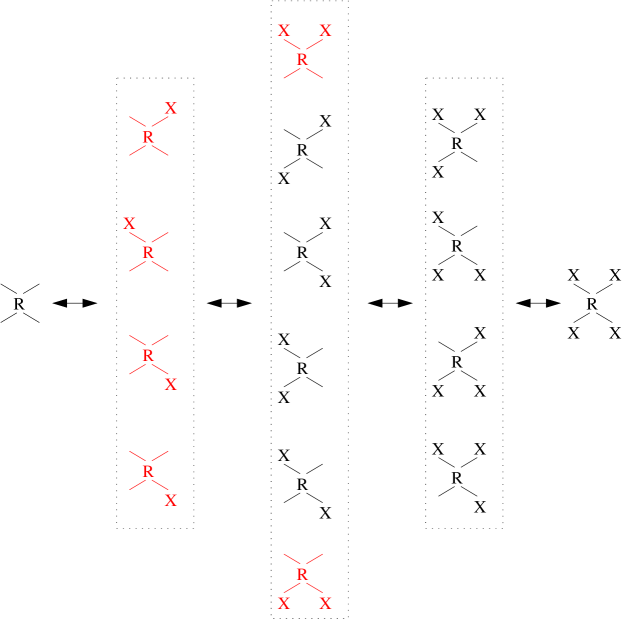
Figure 6: All possible states of repressor-inducer complexes. Here, $R$ and $X$ denote the repressor tetramer and inducer, respectively. The free repressor is on the left. Repressor-inducer complexes containing one free dimer are shown in red.

2.1 States of the lac operon

We denote the free repressor (i.e., repressor not bound to an inducer or operator) and its concentration by $R$ and $r$, respectively. Since the free repressor has 4 inducer binding sites, there are 15 possible repressor-inducer complexes (Fig. 6). We denote the concentrations of repressor-inducer complexes containing 1, 2, 3, and 4 inducer molecules by $r_{1}$, $r_{2}$, $r_{3}$, and $r_{4}$, respectively.

We assume that a repressor dimer can bind to an operator if and only if it contains no inducer. It follows that:

1. In addition to the free repressor, there are six repressor-inducer complexes that can bind to the operator (shown in red in Fig. 6). We denote any inducer-bound repressor with one free dimer by $R^{\prime}$, and the total concentration of such complexes by $r^{\prime}$.

2. Although both $R$ and $R^{\prime}$ can bind to an operator, only operator-bound $R$ can form DNA loops (Fig. 4). Operator-bound $R^{\prime}$ lacks the free dimer necessary for forming a DNA loop (Fig. 2).

These two facts will be crucial for explaining the influence of DNA looping on the induction kinetics.

The lac operon can be in numerous states. There are 14 possible states if we assume that only $R$ can bind to an operator (Fig. 7). Several additional states are feasible because $R^{\prime}$ can also bind to an operator. To enumerate these states systematically, it is convenient to classify them based on the number of repressors bound to an operon. We shall refer to operons containing 0, 1, 2, and 3 repressors as free, unary, binary, and ternary operons, respectively.

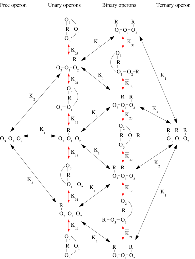
Figure 7: All possible states of the lac operon when only free repressor is permitted to bind to the operators. The black arrows show the reactions which a repressor binds to operator $O_{i}$, and $K_{i}$ denotes the corresponding association constant. The red arrows show the reactions in which a repressor-bound operator, $O_{i}-R$, forms a loop by binding to a free operator $O_{j}$; $K_{ij}$ and $\bar{K}_{ij}$ denote the corresponding association constants for unary and binary operons, respectively.

The operon can be free in only 1 way. We denote the concentration of free operons by $o$.

Unary operons can exist in 9 different states. Six of these correspond to states in which either $R$ or $R^{\prime}$ is bound to one of the operators, say, $O_{i}$. We denote the concentrations of these states by $o_{i}$ and $o_{i^{\prime}}$, respectively. The remaining three states are obtained because free repressor bound to $O_{i}$ can interact with another operator, $O_{j}$, to form a DNA loop. We denote the concentration of such looped states by $o_{\widehat{ij}}$. For example, $o_{\widehat{12}}$ denotes the concentration of the looped state obtained when a free repressor bound to $O_{1}$ interacts with $O_{2}$, or a free repressor bound to $O_{2}$ interacts with $O_{1}$. These definitions imply that

$$u=o_{1}+o_{2}+o_{3}+o_{1^{\prime}}+o_{2^{\prime}}+o_{3^{\prime}}+o_{\widehat{31}}+o_{\widehat{12}}+o_{\widehat{32}},$$ (5)

where $u$ denotes the total concentration of the unary operons.

Binary operons can exist in 18 different states. Twelve of these correspond to the states obtained when $R$ or $R^{\prime}$ bind to any two of the 3 operators. We denote the concentrations of such states by $o_{ij}$, $o_{i^{\prime}j}$, $o_{ij^{\prime}}$, $o_{i^{\prime}j^{\prime}}$, where the indices $i,j$ represent the two operators to which $R$ or $R^{\prime}$ are bound, and the symbol ^′ above an index indicates that $R^{\prime}$, rather than $R$, is bound to the corresponding operator. The remaining 6 complexes are the looped states obtained when the free dimer of an operator-bound free repressor interacts with another free operator. We denote the concentration of such looped complexes by overlaying the symbol $\widehat{}$ on the subscripts representing the two interacting operators. For example, $o_{3\widehat{12}}$ and $o_{3^{\prime}\widehat{12}}$ denote the concentrations of the states in which operator 3 is bound to $R$ and $R^{\prime}$ respectively, and operators 1, 2 interact by looping. It follows that

$$b =\left(o_{31}+o_{3^{\prime}1}+o_{31^{\prime}}+o_{3^{\prime}1^{\prime}}\right)+\left(o_{12}+o_{1^{\prime}2}+o_{12^{\prime}}+o_{1^{\prime}2^{\prime}}\right)$$

$$\quad+\left(o_{32}+o_{3^{\prime}2}+o_{32^{\prime}}+o_{3^{\prime}2^{\prime}}\right)$$

$$\quad+\left(o_{\widehat{31}2}+o_{\widehat{31}2^{\prime}}+o_{3\widehat{12}}+o_{3^{\prime}\widehat{12}}+o_{\widehat{312}}+o_{\widehat{31^{\prime}2}}\right),$$ (6)

where $b$ denotes the total concentration of the binary operons.

Ternary operons can exist in 9 possible states, none of which are looped because loops cannot form in ternary operons. The concentrations of these states are denoted by $o_{\cdot\cdot\cdot}$, where each $\cdot$ contains an integer of the form $i$ or $i^{\prime}$ indicating whether $R$ or $R^{\prime}$ is bound to the $i$-th operator. Evidently

$$t=\left(o_{312}+o_{31^{\prime}2}+o_{312^{\prime}}+o_{31^{\prime}2^{\prime}}\right)+\left(o_{3^{\prime}12}+o_{3^{\prime}1^{\prime}2}+o_{3^{\prime}12^{\prime}}+o_{3^{\prime}1^{\prime}2^{\prime}}\right),$$ (7)

where $t$ denotes the total concentration of the ternary complexes.

2.2 Transcription rate

Oehler et al have postulated that:

1. Binding of the repressor to $O_{1}$ blocks transcription by occluding RNA polymerase (Müller-Hill, 1996, Chap. 1.18).

2. Binding of the repressor to $O_{2}$ has no effect on the transcription rate. This is not because the repressor rarely binds to $O_{2}$: Even if the repressor is overexpressed 90-fold, $O_{2}$-containing cells show no measurable repression (Oehler et al., 1990, Table I). This suggests that $O_{2}$-bound repressor cannot obstruct the movement of RNA polymerase.

3. Binding of the repressor to $O_{3}$ does not block transcription. It merely reduces (deactivates) the transcription rate by preventing CAP from binding to the repressor.
   This hypothesis is based on the following argument. If repressor-bound $O_{3}$ blocked transcription, the repression in $O_{3}$-containing cells would increase monotonically with the repressor level. However, if the repressor is overexpressed in these cells, the repression saturates at 25 (Oehler et al., 1994, p. 3351).

These postulates imply that the transcription rate is proportional to

$$T\equiv\frac{o}{o_{t}}+\left(\frac{o_{2}}{o_{t}}+\frac{o_{2^{\prime}}}{o_{t}}\right)+d\left(\frac{o_{3}}{o_{t}}+\frac{o_{3^{\prime}}}{o_{t}}+\frac{o_{32}}{o_{t}}+\frac{o_{3^{\prime}2}}{o_{t}}+\frac{o_{32^{\prime}}}{o_{t}}+\frac{o_{3^{\prime}2^{\prime}}}{o_{t}}+\frac{o_{\widehat{32}}}{o_{t}}\right),$$

where $d<1$ is a parameter accounting for deactivation of transcription by repressor-bound $O_{3}$.

2.3 Governing equations

To determine the concentrations of the various states, we assume that

1. The total concentrations of the repressor and operator, denoted $r_{t}$ and $o_{t}$, are constant.

2. The system is in thermodynamic equilibrium, and satisfies the principle of detailed balance (i.e., the net rate of every reaction is zero).

3. The binding of $R$ or $R^{\prime}$ to an operator does not affect the affinity of the remaining free operators for $R$ and $R^{\prime}$. Hence, one can define $K_{i}$ and $K_{i^{\prime}}$ as the association constants for the binding of $R$ and $R^{\prime}$ to $O_{i}$, regardless of the state of the remaining operators. Evidently, $K_{i^{\prime}}=K_{i}/2$, since $R$ contains two inducer-free dimers, both of which can bind to $O_{i}$, whereas $R^{\prime}$ contains only 1 inducer-free dimer.
   We denote the association constants for formation of unary and binary loops by $K_{ij}$ and $\bar{K}_{ij}$, respectively (Fig. 7).

4. All four inducer-binding sites on the repressor are identical and independent. We denote the association constant for binding of an inducer to any one of these sites by $K_{x}$.

Assumption 1 implies the conservation relations

$$\left(r+r_{1}+r_{2}+r_{3}+r_{4}\right)+u+2b+3t =r_{t},$$ (8)

$$o+u+b+t =o_{t},$$ (9)

where the factors 2 and 3 in (8) account for the fact that the binary and ternary operons contain 2 and 3 repressors, respectively.

Assumptions 2 and 3 yield the equilibrium relations

$\begin{array}[]{ccc}o_{i}=K_{i}or&o_{i^{\prime}}=\frac{1}{2}K_{i}or^{\prime}&o_{\widehat{ij}}=K_{ij}K_{i}or=K_{ji}K_{j}or,\\ o_{ij}=K_{i}K_{j}or^{2}&o_{i^{\prime}j}=o_{ij^{\prime}}=\frac{1}{2}K_{i}K_{j}orr^{\prime}&o_{i^{\prime}j^{\prime}}=\frac{1}{4}K_{i}K_{j}o\left(r^{\prime}\right)^{2},\end{array}$

and

$\begin{array}[]{cc}o_{\widehat{31}2}=K_{2}K_{3}\bar{K}_{31}or^{2}=K_{2}K_{1}\bar{K}_{13}or^{2}&o_{\widehat{31}2^{\prime}}=\frac{1}{2}K_{2}K_{3}\bar{K}_{31}orr^{\prime}=\frac{1}{2}K_{2}K_{1}\bar{K}_{13}orr^{\prime},\\ o_{3\widehat{12}}=K_{3}K_{1}\bar{K}_{12}or^{2}=K_{3}K_{2}\bar{K}_{21}or^{2}&o_{3^{\prime}\widehat{12}}=\frac{1}{2}K_{3}K_{1}\bar{K}_{12}orr^{\prime}=\frac{1}{2}K_{3}K_{2}\bar{K}_{21}orr^{\prime},\\ o_{\widehat{312}}=K_{1}K_{3}\bar{K}_{32}or^{2}=K_{1}K_{2}\bar{K}_{23}or^{2}&o_{\widehat{31^{\prime}2}}=\frac{1}{2}K_{1}K_{3}\bar{K}_{32}or^{2}=\frac{1}{2}K_{1}K_{2}\bar{K}_{23}or^{2},\\ o_{312}=K_{1}K_{2}K_{3}or^{3}&o_{3^{\prime}12}=o_{31^{\prime}2}=o_{312^{\prime}}=\frac{1}{2}K_{1}K_{2}K_{3}or^{2}r^{\prime},\\ o_{3^{\prime}1^{\prime}2^{\prime}}=\frac{1}{8}K_{1}K_{2}K_{3}o\left(r^{\prime}\right)^{3}&o_{31^{\prime}2^{\prime}}=o_{3^{\prime}12}=o_{3^{\prime}1^{\prime}2}=\frac{1}{4}K_{1}K_{2}K_{3}or\left(r^{\prime}\right)^{2},\end{array}$

where the concentrations of the looped species have two representations (e.g., $o_{\widehat{ij}}=K_{ij}K_{i}or=K_{ji}K_{j}or$) because these species can be formed by two different pathways (Fig. 7).

These equilibrium relations imply that eqs. (5–7) can be rewritten as

$$u =o\left[\left(K_{1}+K_{2}+K_{3}\right)\left(r+\frac{r^{\prime}}{2}\right)+\left(K_{1}K_{12}+K_{1}K_{13}+K_{2}K_{23}\right)r\right],$$ (10)

$$b =o\left[\left(K_{1}K_{2}+K_{1}K_{3}+K_{2}K_{3}\right)\left(r+\frac{r^{\prime}}{2}\right)^{2}\right.$$ (11)

$$\qquad\qquad+K_{1}\left(K_{2}\bar{K}_{23}+K_{2}\bar{K}_{13}+K_{3}\bar{K}_{12}\right)\left(r+\frac{r^{\prime}}{2}\right),$$

$$t =o\cdot K_{1}K_{2}K_{3}\left(r+\frac{r^{\prime}}{2}\right)^{3}.$$ (12)

Assumptions 2 and 4 imply that the total concentration of all the complexes shown in Fig. 6 is given by

$$r+r_{1}+r_{2}+r_{3}+r_{4} =r\left(1+K_{x}x\right)^{4},$$ (13)

and the total concentration of repressor-inducer complexes with one free dimer is

$$r^{\prime} =r\left(4K_{x}x+2K_{x}^{2}x^{2}\right)\Rightarrow r+\frac{r^{\prime}}{2}=r\left(1+K_{x}x\right)^{2}.$$ (14)

These two equations follow immediately from statistical thermodynamic theory (Ackers et al., 1982).

Substituting (10–14) in (8)–(9) yields the two governing equations

$$r\left(1+K_{x}x\right)^{4}$$

$$+or\left[\left(K_{1}+K_{2}+K_{3}\right)\left(1+K_{x}x\right)^{2}+K_{1}K_{12}+K_{1}K_{13}+K_{2}K_{23}\right]$$

$$+2or^{2}\left[\left(K_{1}K_{2}+K_{1}K_{3}+K_{2}K_{3}\right)\left(1+K_{x}x\right)^{4}\right.$$

$$\left.+K_{1}\left(\bar{K}_{23}+\bar{K}_{13}+\bar{K}_{12}\right)\left(1+K_{x}x\right)^{2}\right]+3or^{3}\left(1+K_{x}x\right)^{6}K_{1}K_{2}K_{3} =r_{t},$$ (15)

$$o+or\left[\left(K_{1}+K_{2}+K_{3}\right)\left(1+K_{x}x\right)^{2}+K_{1}K_{12}+K_{1}K_{13}+K_{2}K_{23}\right]$$

$$+or^{2}\left[\left(K_{1}K_{2}+K_{1}K_{3}+K_{2}K_{3}\right)\left(1+K_{x}x\right)^{4}\right.$$

$$\left.+K_{1}\left(\bar{K}_{23}+\bar{K}_{13}+\bar{K}_{12}\right)\left(1+K_{x}x\right)^{2}\right]+3or^{3}K_{1}K_{2}K_{3}\left(1+K_{x}x\right)^{6} =o_{t},$$ (16)

containing the 3 variables, $r,o,x$.

The equilibrium relations imply that

$$T =\frac{o}{o_{t}}\left[1+K_{2}r\left(1+K_{x}x\right)^{2}+d\left\{K_{3}r\left(1+K_{x}x\right)^{2}\right.\right.$$

$$\qquad\qquad\left.\left.+K_{2}K_{3}r^{2}\left(1+K_{x}x\right)^{4}+K_{2}K_{23}r\right\}\right].$$

Eqs. (15)–(16) yield $o$ and $r$ as a function of $x$, which can be substituted in the above expression to obtain $T$ as a function of the inducer concentration.

2.4 Scaled equations

It is convenient to define the dimensionless variables

$$\rho\equiv\frac{r}{r_{t}},\nu\equiv\frac{o}{o_{t}},\chi\equiv K_{x}x,$$

and the dimensionless parameters

$$\kappa_{i} \equiv K_{i}r_{t},\;i=1,2,3,$$

$$\alpha_{1} \equiv\kappa_{1}+\kappa_{2}+\kappa_{3},$$

$$\widehat{\alpha}_{1} \equiv\kappa_{1}K_{12}+\kappa_{1}K_{13}+\kappa_{2}K_{23},$$

$$\alpha_{2} \equiv\kappa_{1}\kappa_{2}+\kappa_{1}\kappa_{3}+\kappa_{2}\kappa_{3},$$

$$\widehat{\alpha}_{2} \equiv\kappa_{1}\left(\kappa_{2}\bar{K}_{23}+\kappa_{2}\bar{K}_{13}+\kappa_{3}\bar{K}_{12}\right),$$

$$\alpha_{3} \equiv\kappa_{1}\kappa_{2}\kappa_{3},$$

$$\omega \equiv\frac{o_{t}}{r_{t}}.$$

The transcription rate is then proportional to

$$T =\nu\left[1+\kappa_{2}\rho(1+\chi)^{2}+d\left\{\kappa_{3}\rho(1+\chi)^{2}\right\}\right.$$

$$\qquad\qquad\qquad\left.\left.+\kappa_{2}\kappa_{3}\rho^{2}(1+\chi)^{4}+\kappa_{2}K_{23}\rho\right\}\right]$$ (17)

and eqs. (15)–(16) become

$$\rho\left(1+\chi\right)^{4}+\omega\nu\left[\rho f_{1}(\chi)+2\rho^{2}f_{2}(\chi)+3\rho^{3}f_{3}(\chi)\right] =1,$$ (18)

$$\nu\left[1+\rho f_{1}(\chi)+\rho^{2}f_{2}(\chi)+\rho^{3}f_{3}(\chi)\right] =1,$$ (19)

where

$$f_{1}(\chi) \equiv\alpha_{1}\left(1+\chi\right)^{2}+\widehat{\alpha}_{1},$$

$$f_{2}(\chi) \equiv\alpha_{2}\left(1+\chi\right)^{4}+\widehat{\alpha}_{2}\left(1+\chi\right)^{2},$$

$$f_{3}(\chi) \equiv\alpha_{3}\left(1+\chi\right)^{6}.$$

As we show below, the parameters, $\alpha_{i}$ and $\widehat{\alpha}_{i}$, are related to the repression due to repressor-operator binding and DNA looping, respectively. The parameter, $\omega$, is typically quite small. In wild-type Escherichia coli, $\omega\approx 0.2$ since each cell contains 10 repressor molecules and no more than 2 operators (Müller-Hill, 1996, Chap. 3.2). In many experiments, the repressor is overexpressed (>50 molecules per cell), so that $\omega<0.02$.

3 Results

In what follows, we shall determine the values of $\alpha_{i}$ and $\widehat{\alpha}_{i}$ by appealing to the repression data. It is therefore useful to express the repression in terms of the model.

To this end, we begin by observing that during exponential growth in the presence of IPTG and glycerol, the mass balance for $\beta$-galactosidase yields

$$\frac{de}{dt}=r_{e}(x)-\left(r_{g}+k_{e}^{-}\right)e=0\Rightarrow e=\frac{r_{e}(x)}{r_{g}+k_{e}^{-}},$$

where $x$ is the concentration of IPTG, $r_{e}(x)$ is the corresponding specific rate of $\beta$-galactosidase synthesis, $r_{g}$ is the maximum specific growth rate on glycerol, and $k_{e}^{-}$ is the rate constant for $\beta$-galactosidase degradation. Since $r_{g}+k_{e}^{-}$ is a fixed parameter, $e$ is proportional to $r_{e}$, and (3) becomes

$$\mathcal{R}=\frac{\left.r_{e}(x)\right|_{x\rightarrow\infty}}{r_{e}(0)}.$$

It follows from (17) that

$$\mathcal{R}=\frac{1}{T(0)}=\frac{1}{\nu(0)\left[1+\kappa_{2}+d\left(\kappa_{3}+\kappa_{2}\kappa_{3}+\kappa_{2}K_{23}\right)\right]},$$ (20)

where we have assumed that $\rho(0)=1$, and at large inducer concentrations, $\rho=0,\nu=1$.

Oehler et al measured the repression in the presence of various combinations of operators (Table 1). We shall distinguish these cases by using subscripts to denote the particular combination of operators being considered. Specifically, $\mathcal{R}_{i}$ will denote the repression in cells containing only the $i$-th operator, $\mathcal{R}_{ij}$ will denote the repression in cells containing the $i$-th and $j$-th operators, and $\mathcal{R}_{312}$ will denote the repression in cells containing all 3 operators.

We begin by considering the special cases in which there is no DNA looping, and then proceed to the more general case that accounts for DNA looping.

3.1 No DNA looping

In the experiments, DNA looping was abolished by deleting the auxiliary operators or mutating the locus for the oligomerization domain of the repressor. Here, we consider the first case. The case of mutant dimers is discussed in Appendix A.

In the absence of the auxiliary operators, $\kappa_{2}=\kappa_{3}=0$, so that

$$\alpha_{1}=\kappa_{1},\;\widehat{\alpha}_{1}=\alpha_{2}=\widehat{\alpha}_{1}=\alpha_{3}=0,$$ (21)

and eqs. (17)–(19) become $T=\nu,$ and

$$\rho\left(1+\chi\right)^{4}+\omega\nu\rho\kappa_{1}\left(1+\chi\right)^{2} =1,$$ (22)

$$\nu\left[1+\rho\kappa_{1}\left(1+\chi\right)^{2}\right] =1.$$ (23)

We can get $\nu(\chi)$ from these equations by eliminating $\rho$ and solving the resulting quadratic. However, this solution is cumbersome and offers little insight. Instead, since $\omega$ is small, we appeal to perturbation theory (Appendix B), which formalizes the following physical argument.

Since the number of operons per cell is small compared to the number of repressors per cell, one can assume, as a first approximation, that the fraction of operon-bound repressors is negligibly small compared to the fraction of free repressors, i.e., $\omega=0$. Equations (22)–(23) then yield the approximate zeroth-order solution

$$\rho_{0} =\frac{1}{\left(1+\chi\right)^{4}},$$ (24)

$$\nu_{0} =\frac{1}{1+\kappa_{1}\rho_{0}\left(1+\chi\right)^{2}}.$$ (25)

To estimate the error of the approximation, we acknowledge that the fraction of operon-bound repressors is small but not zero. We assume furthermore that this fraction can be estimated by the expression, $\omega\nu_{0}\rho_{0}\kappa_{1}\left(1+\chi\right)^{2}$, and solve the resulting equations

$$\rho\left(1+\chi\right)^{4}+\omega\nu_{0}\rho_{0}\kappa_{1}\left(1+\chi\right)^{2} =1,$$

$$\nu\left[1+\rho\kappa_{1}\left(1+\chi\right)^{2}\right] =1,$$

to obtain the improved first-order solution

$$\rho =\rho_{0}\left[1-\omega\left(1-\nu_{0}\right)\right]+O(\omega^{2}),$$ (26)

$$\nu =\nu_{0}\left[1+\omega\left(1-\nu_{0}\right)^{2}\right]+O(\omega^{2}).$$ (27)

It follows from (27) that the relative error of $\nu_{0}$ is approximately

$$\frac{\nu-\nu_{0}}{\nu}=\frac{\omega\left(1-\nu_{0}\right)^{2}}{1+\omega\left(1-\nu_{0}\right)^{2}}<\frac{\omega}{1+\omega}.$$

Since, $\omega\lesssim 0.2$, the zeroth-order solution is accurate to within $100\omega/(1+\omega)\approx 15$% in wild-type cells, and even more accurate in repressor-overexpressed cells. Henceforth, we shall assume that eqs. (24)–(25) are a good approximation to the exact solution, so that

$$T(\chi)=\nu(\chi)\approx\frac{1}{1+\kappa_{1}/\left(1+\chi\right)^{2}},$$ (28)

which is formally identical to eq. (1) with $K_{x,1}=2K_{x},$ $K_{x,1}K_{x,2}=K_{x}^{2}$, the special case of the Yagil & Yagil model corresponding to identical and independent inducer-binding sites (Yagil and Yagil, 1971, p 19).

It follows from (28) that induction is cooperative even in the absence of DNA looping. Indeed, since $T(\chi)$ has a unique inflection point at $\chi=\sqrt{\alpha_{1}/3}-1$, $T=1/4$, the kinetics are cooperative for all inducer concentrations such that $0\leq T\leq 1/4$. In the particular case of Fig. 5a, the kinetics are cooperative for all inducer concentrations in the range 0–50 $\mu$M, which is significantly higher than the 0–5 $\mu$M range reported in Oehler et al., 2006, based upon visual inspection of the curve.

Figure 8: Estimation of $\kappa_{1}$ and $\kappa_{3}$ by fitting the repression data from Oehler et al., 1990, Table I, and Oehler et al., 1994, Fig. 1, to eqs. (29–30).

The parameters, $\kappa_{1}$, $K_{x1}$, can be estimated from the induction curve by observing that (28) implies

$$\sqrt{\frac{T}{1-T}}=\frac{1}{\sqrt{\kappa_{1}}}+\frac{K_{x}}{\sqrt{\kappa_{1}}}x.$$

If the model is correct, a plot of $\sqrt{T/(1-T)}$ vs $x$ will be a straight line, and $\kappa_{1},K_{x}$ can be estimated from the slope and $y$-intercept. The induction curve shown in Fig. 5a yields a straight line with $\kappa_{1}=227$ and $K_{x}^{-1}=6.7$ $\mu\textnormal{M}$ (Oehler et al., 2006, Fig. 4B).

The value of $\kappa_{1}$ can also be estimated from the repression data. Indeed, it follows from (28) that

$$\mathcal{R}_{1}=\frac{1}{T(0)}=1+\kappa_{1}.$$ (29)

Fitting the repression at various overexpression levels to this equation yields $\kappa_{1}=30$ for wild-type cells (Fig. 8a). This is $\sim$7-fold lower than the value estimated above because the induction curve was obtained with repressor-overexpressed cells.

Although eq. (25) was derived for cells containing the main operator $O_{1}$, analogous expressions are obtained for cells containing an auxiliary operator, i.e., $\nu=1/\left[1+\kappa_{i}/(1+\chi)^{2}\right]$ for $i=2,3$. Equation (20) then implies that the repression in $O_{3}$-containing cells is

$$\mathcal{R}_{3}=\frac{1+\kappa_{3}}{1+d\kappa_{3}},$$

which captures the deactivation effect noted by Oehler et al: $\mathcal{R}_{3}$ increases with the repressor level until it saturates $1/d$. However, the data shows no evidence of this saturation even if the repressor is overexpressed 90-fold (Fig. 8b). Nonlinear regression of the data using the above expression yields the best-fit parameters, $d=0$ and $\kappa_{3}=0.24$ for wild-type cells. It is conceivable that $d$ is positive, but so small that $d\kappa_{3}\ll 1$ for the overexpression levels shown in Fig. 8b. Henceforth, we shall assume that $d=0$, and

$$\mathcal{R}_{3}=1+\kappa_{3},$$ (30)

a relation that is valid up to an overexpression level of 90.

Unlike $\kappa_{1}$ and $\kappa_{3}$, the parameter, $\kappa_{2}$, cannot be calculated from the repression data for $O_{2}$-containing cells because they show no repression even if the repressor is overexpressed 90-fold. This property is implicit in the model as well. Indeed, (20) implies that

$$\mathcal{R}_{2}=\frac{1}{\nu(0)(1+\kappa_{2})}=\frac{1+\kappa_{2}}{1+\kappa_{2}}=1,$$

regardless of the repressor level. Evidently, this reflects the fact that $O_{2}$-bound repressor does not block RNA polymerase.

3.2 DNA looping

In this case, the full system of eqs. (18)–(19) must be solved for $\nu$ and $\rho$. Perturbation theory yields the zeroth-order solution

$$\rho_{0} =\frac{1}{\left(1+\chi\right)^{4}},$$ (31)

$$\nu_{0} =\frac{1}{1+\rho_{0}f_{1}(\chi)+\rho_{0}^{2}f_{2}(\chi)+\rho_{0}^{3}f_{3}(\chi)}.$$ (32)

It is evident from (32) that $\rho_{0}f_{1}(\chi)$, $\rho_{0}^{2}f_{2}(\chi)$, and $\rho_{0}^{3}f_{3}(\chi)$ are the concentrations of the unary, binary, and ternary operons, respectively, relative to the concentration of the free operons. We shall constantly appeal to this fact below.

The zeroth-order solution is a good approximation to the exact solution. Indeed, the first order solution is given by (Appendix B)

$$\rho =\rho_{0}\left(1-\omega\Omega_{0}\right)+O(\omega^{2}),$$

$$\nu =\nu_{0}\left(1+\omega\Omega_{0}^{2}\right)+O(\omega^{2}),$$

where

$$\Omega_{0}\equiv\frac{\rho_{0}f_{1}(\chi)+2\rho_{0}^{2}f_{2}(\chi)+3\rho_{0}^{3}f_{3}(\chi)}{1+\rho_{0}f_{1}(\chi)+\rho_{0}^{2}f_{2}(\chi)+3\rho_{0}^{3}f_{3}(\chi)},$$ (33)

and the relative error of $\nu_{0}$ is approximately

$$\frac{\nu-\nu_{0}}{\nu}=\frac{\omega\Omega_{0}^{2}}{1+\omega\Omega_{0}^{2}}.$$

The above interpretation of the terms, $\rho_{0}^{i}f_{i}(\chi),i=1,2,3$, implies that $\Omega_{0}$ is the average number of repressors per operon, and hence, can have any value between 0 and 3. At large inducer concentrations, $\Omega_{0}\approx 0$, and the error is guaranteed to be vanishingly small. At low inducer concentrations, $\Omega_{0}$ can exceed 1, provided the fraction of binary and ternary operons is sufficiently large. However, we show below that in wild-type cells, $\Omega_{0}$ is close to 1 (Fig. 13a). In repressor-overexpressed cells, $\Omega_{0}$ can approach 3, but $\omega$ is so small that the relative error of $\nu_{0}$ does not exceed 20% (Fig. 17). The zeroth-order solution is therefore a good approximation at all repressor levels and inducer concentrations.

Substituting (31) in (32) and (17) with $d=0$ yields

$$\nu_{0} =\frac{1}{1+\frac{\alpha_{1}}{\left(1+\chi\right)^{2}}+\frac{\widehat{\alpha}_{1}}{\left(1+\chi\right)^{4}}+\frac{\alpha_{2}}{\left(1+\chi\right)^{4}}+\frac{\widehat{\alpha}_{2}}{\left(1+\chi\right)^{6}}+\frac{\alpha_{3}}{\left(1+\chi\right)^{6}}},$$ (34)

$$T =\nu_{0}\left[1+\frac{\kappa_{2}}{(1+\chi)^{2}}\right],$$ (35)

which shows that in the presence of DNA looping, the induction rate is formally different from (28). It turns out, however, that in wild-type lac, the parameter values are such that several terms in the above expresssions are negligibly small. To see this, it is useful to define

$$\phi_{i} (\chi)\equiv\frac{\alpha_{i}}{\left(1+\chi\right)^{2i}},\;i=1,2,3,$$ (36)

$$\widehat{\phi}_{i} (\chi)\equiv\frac{\widehat{\alpha}_{i}}{\left(1+\chi\right)^{2(i+1)}},\;i=1,2,$$ (37)

and rewrite (34) as

$$\nu_{0}=\frac{1}{1+\phi_{1}(\chi)+\widehat{\phi}_{1}(\chi)+\phi_{2}(\chi)+\widehat{\phi}_{2}(\chi)+\phi_{3}(\chi)}.$$ (38)

Evidently, $\phi_{i}(\chi)$ and $\widehat{\phi}_{i}(\chi)$ are the relative concentrations of the non-looped and looped operons containing $i$ repressors (measured relative to the concentration of free operons). In particular, the parameters, $\alpha_{i}=\phi_{i}(0)$ and $\widehat{\alpha}_{i}=\widehat{\phi}_{i}(0)$, are the relative concentrations of these operons in the absence of the inducer.

Figure 9: Estimation of $\kappa_{2}$, $K_{12}$, $K_{13}$, and $K_{23}$ by fitting the repression data from Oehler et al., 1990, Table I and Oehler et al., 1994, Figs 4–5 to eqs. (40) and (42). The values of $\mathcal{R}_{31}$ and $\mathcal{R}_{312}$ at 90-fold overexpression are lower bounds for the repression. The true repression levels are too high to be measured accurately.

We begin by determining the wild-type values of $\alpha_{i}$ and $\widehat{\alpha}_{i}$. The above estimates of $\kappa_{1}$, $\kappa_{2}$, and $\kappa_{3}$ imply that $\alpha_{1}=31$, $\alpha_{2}=19$, and $\alpha_{3}=3$. To find the remaining parameters, $\widehat{\alpha}_{1},\widehat{\alpha}_{2}$, observe that since

$$\mathcal{R}_{312}=\frac{1}{T(0)}=\frac{1+\alpha_{1}+\widehat{\alpha}_{1}+\alpha_{2}+\widehat{\alpha}_{2}+\alpha_{3}}{1+\kappa_{2}},$$ (39)

the repression in cells containing pairs of operators are given by the expressions

$$\mathcal{R}_{12} =\frac{1+\kappa_{1}+\kappa_{2}+\kappa_{1}K_{12}+\kappa_{1}\kappa_{2}}{1+\kappa_{2}},$$ (40)

$$\mathcal{R}_{32} =\frac{1+\kappa_{2}+\kappa_{3}+\kappa_{2}K_{23}+\kappa_{2}\kappa_{3}}{1+\kappa_{2}},$$ (41)

$$\mathcal{R}_{31} =1+\kappa_{1}+\kappa_{3}+\kappa_{1}K_{13}+\kappa_{1}\kappa_{3}.$$ (42)

Fitting the repression data obtained at various overexpression levels to these equations yields the estimates, $\kappa_{2}=0.38$, $K_{12}=32$, $K_{13}=15$, $K_{23}=2.5$ (Fig. 9), which imply that

$$\widehat{\alpha}_{1}\equiv\kappa_{1}K_{12}+\kappa_{1}K_{13}+\kappa_{2}K_{23}=1420.$$

Since the measured value of $\mathcal{R}_{312}$ is 1300, eq. (39) implies that $\widehat{\alpha}_{2}=322$.

These parameter values imply that in wild-type cells, the induction rate is much simpler than (35). To see this, observe that in the absence of the inducer, the relative concentrations of binary and ternary operons are small compared to the relative concentrations of free and unary operons, i.e.,

$$\alpha_{2}+\widehat{\alpha}_{2}+\alpha_{3}\ll 1+\alpha_{1}+\widehat{\alpha}_{1}.$$ (43)

Now, eqs. (36–37) imply that in the presence of the inducer, the relative concentrations of the binary and ternary operons decrease with the inducer concentration at a rate as fast, or even faster, than the corresponding rate for the looped unary operons. It follows that even in the presence of the inducer, the relative concentrations of the binary and ternary operons remain negligibly small compared to the relative concentrations of the unary and free operons, i.e., the relation

$$\phi_{2}(\chi)+\widehat{\phi}_{2}(\chi)+\phi_{3}(\chi)\ll 1+\phi(\chi)+\widehat{\phi}_{1}(\chi)$$

is true for all $\chi\geq 0$. The fraction of free operons in wild-type lac is therefore well-approximated by the simpler expression

$$\nu_{0} \approx\frac{1}{1+\phi_{1}(\chi)+\widehat{\phi}_{1}(\chi)}.$$ (44)

A similar argument shows that in the absence of the inducer, $\kappa_{2}/(1+\chi)^{2}$, the relative concentration of $O_{2}$-bound operons, is 0.38, and (35) implies that almost 1/3 of the transcription occurs from $O_{2}$-bound operons. However, $\kappa_{2}/(1+\chi)^{2}$ decreases so rapidly with the inducer concentration that it is already below 0.2 at $\chi=0.5$. Thus, the transcription rate of wild-type lac is well-approximated by the expression

$$T(\chi)\approx\nu_{0}(\chi)=\frac{1}{1+\alpha_{1}/\left(1+\chi\right)^{2}+\widehat{\alpha}_{1}/\left(1+\chi\right)^{4}}$$ (45)

for all but a negligibly small range of inducer concentrations. This expression is simpler than (35), but formally different from (28). The physical reason for this will be discussed shortly.

The parameter values also imply that in the absence of the inducer, the relative concentrations of the free and non-looped unary operons are negligibly small compared to relative concentration of looped unary operons, i.e.,

$$1+\alpha_{1}\ll\widehat{\alpha}_{1}.$$

It follows that in wild-type cells, the repression is exerted almost entirely by the looped unary operons, i.e.,

$$\mathcal{R}_{312}\approx\frac{\widehat{\alpha}_{1}}{1+\kappa_{2}}\approx\frac{\kappa_{1}\left(K_{12}+K_{13}\right)}{1+\kappa_{2}}.$$ (46)

This equation explains an important trend in Table 1. Specifically, the addition of only one of the auxiliary operators to the main operator increases the repression dramatically (25- to 40-fold) because $K_{12},K_{13}\gg 1$. However, addition of the second auxiliary operator provokes no more than a 2- or 3-fold increase because the magnitudes of $K_{12}$ and $K_{13}$ are comparable.

Comparison of (28) and (45) shows that the induction kinetics are qualitatively different in the presence of DNA looping precisely because $\widehat{\phi}_{1}(\chi)$ decreases faster than $\phi_{1}(\chi)$. The physical reason for this is as follows. Looped unary states can form only if free repressor binds to an operator, whereas non-looped unary states can form if free or inducer-bound repressor binds to an operator. More precisely, eqs. (10) and (14) show that the relative concentrations of looped and non-looped unary operons are proportional to $r$ and $r+r^{\prime}/2=r(1+\chi)^{2}$, respectively. Since $r$ is proportional to $(1+\chi)^{-4}$, $\widehat{\phi}_{1}(\chi)$ and $\phi_{1}(\chi)$ decrease at the rates $(1+\chi)^{-4}$ and $(1+\chi)^{-2}$, respectively.

Figure 10: Analysis of the data for strains BB20 lac${}_{3}^{-}$ ($\blacklozenge$), 2001c ($\bigstar$), and 15TAU lac${}_{2}^{-}$ ($\blacksquare$) (Overath, 1968, Fig. 1). (a) The $\left[T/(1-T)\right]^{1/2}$ vs. $x$ plots are not straight lines. The slopes decrease significantly at low inducer concentrations. (b) The $\left[T/(1-T)\right]^{1/4}$ vs. $x$ plots are linear at low inducer concentrations. The black, red, and green lines are fits obtained from the data for IPTG concentrations below 20 $\mu$M.

Analysis of the data confirms that DNA looping produces a qualitative change in the kinetics, which cannot be captured by quantitative adjustment of the parameters in eq. (25). If the data were consistent with (25), the $[T/(1-T{)]}^{1/2}$ vs. $x$ plots would be straight lines. However, construction of these plots for three different strains of E. coli yields not straight lines, but curves with conspicuously small slopes at low inducer concentrations (Fig. 10a).

Table 2: Parameter values of eq. (45) estimated from the induction curves for 6 different strains of E. coli.

Strain	$K_{x}^{-1}$ ($\mu$M)	$\widehat{\alpha}_{1}$	$\alpha_{1}$	Reference
BB20 lac${}_{3}^{-}$	16.3	1834	62	Overath, 1968, Fig. 1
2001c	26.2	741	12	Overath, 1968, Fig. 1
15 TAU lac${}_{2}^{-}$	44.2	89	0	Overath, 1968, Fig. 1
600Coc$y_{1}^{-}$	17.5	13	0	Overath, 1968, Fig. 1
W3102$i^{t}$	3.0	66	7	Gilbert and Müller-Hill, Fig. 1
BMH8117 $\lambda$Ewt123	10.9	4921	219	Oehler et al., 2006, Fig. 1A

The reason for the nonlinearity of the $[T/(1-T)]^{1/2}$ vs. $x$ plot becomes evident if eq. (45) is rewritten as

$$\frac{1}{T}-1=\frac{\widehat{\alpha}_{1}}{\left(1+\chi\right)^{4}}+\frac{\alpha_{1}}{\left(1+\chi\right)^{2}}.$$

Since $\widehat{\alpha}_{1}\sim 50\alpha_{1}$ in wild-type lac, the first term, which accounts for the repression due to looped unary operons, dominates at sufficiently low inducer concentrations, $\chi\ll\sqrt{\widehat{\alpha}_{1}/\alpha_{1}}-1\approx 6$. At these low concentrations, $[T/(1-T)]^{1/4}$ vs. $x$ plots should be straight lines because

$$\left(\frac{T}{1-T}\right)^{1/4}\approx\frac{1}{\widehat{\alpha}_{1}^{1/4}}+\left(\frac{K_{x}}{\widehat{\alpha}_{1}^{1/4}}\right)x.$$

The experimental data for 3 different strains of E. coli shows that this is indeed the case (Fig. 10b). To be sure, the $[T/(1-T)]^{1/2}$ vs. $x$ plots are also straight lines at sufficiently large inducer concentrations (Fig. 10a). This is because when $\chi\gg\sqrt{\widehat{\alpha}_{1}/\alpha_{1}}-1$, the non-looped unary states dominate, so that

$$\left(\frac{T}{1-T}\right)^{1/2}\approx\frac{1}{\alpha_{1}^{1/2}}+\left(\frac{K_{x}}{\alpha_{1}^{1/2}}\right)x.$$

However, neither plot can be linear over the entire range of inducer concentrations.

Eq. (45) provides good fits to the experimental data (Figs. 5c and 11). The parameter values for these fits, shown in Table 2, were estimated as follows. If sufficient data was available at low inducer concentrations (Fig. 11), $\widehat{\alpha}_{1}$ and $K_{x}$ were estimated from the slopes and intercepts of the $[T/(1-T)]^{1/4}$ vs. $x$ plots. The value of $\alpha_{1}$ was then determined by one-parameter nonlinear regression of the data (MATLAB, LSQNONLIN). If accurate data was not available at low concentrations (Fig. 5c), all three parameter values were obtained by nonlinear regression of the data.

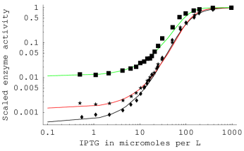
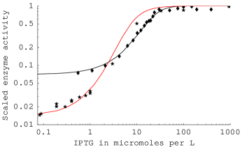
Figure 11: Fits of the data from Overath, 1968 and Gilbert and Müller-Hill, 1966 for: (a) BB20 lac${}_{3}^{-}$ ($\blacklozenge$), 2001c ($\bigstar$), and 15TAU lac${}_{2}^{-}$ ($\blacksquare$). (b) Operator-constitutive strain 600Co^c$y_{1}^{-}$ ($\blacklozenge$), and tight-binding strain W3102 ($\bigstar$). The data was fitted with eq. (45) and the parameter values in Table 2.

In wild-type cells, the binary and ternary operons were neglected by appealing to (36)–(37) and (43). The latter relation is not valid for repressor-overexpressed cells. This is because $\alpha_{j},\widehat{\alpha}_{j}$ are proportional to $(r_{t})^{j}$. Hence, as the repressor level increases, $\alpha_{2},\widehat{\alpha}_{2},\alpha_{3}$ increase much faster than $\alpha_{1},\widehat{\alpha}_{1}$, and at sufficiently large repressor levels,

$$\alpha_{3}\gg\alpha_{2},\widehat{\alpha}_{2}\gg\alpha_{1},\widehat{\alpha}_{1}\gg 1,$$ (47)

i.e., almost all the operons are in the ternary state. Fig. 12a shows that in the absence of the inducer, $\Omega_{0}\approx 1$ in wild-type cells, but increases to $\sim$3 in cells containing $\sim$500 times the wild-type repressor levels. In vitro data provides direct evidence of this increase in $\Omega_{0}$. When DNA fragments, containing two appropriately spaced lac operators, are exposed to increasing repressor levels, there is a perceptible increase in the concentration of binary non-looped complexes (Fig. 12b). In vivo data also suggests that $\Omega_{0}$ increases in repressor-overexpressed cells. Oehler et al found similar repression levels in two different strains of E. coli containing high levels (900 molecules per cell) of the wild-type tetrameric and mutant dimeric repressor, respectively (Oehler et al., 1990, Table I). They argued that this is because at such high repressor levels, most of the operons are in the ternary state. Since ternary operons cannot form loops even in cells containing the tetrameric repressor, the repression levels are similar in both cell types. More precisely, (47) and (52) imply that

$$\frac{\left.\mathcal{R}_{312}\right|_{\textnormal{dimer}}}{\left.\mathcal{R}_{312}\right|_{\textnormal{tetramer}}}=\frac{\left(1+\alpha_{1}/2+\alpha_{2}/4+\alpha_{3}/8\right)/\left(1+\kappa_{2}/2\right)}{\left(1+\alpha_{1}+\widehat{\alpha}_{1}+\alpha_{2}+\widehat{\alpha}_{2}+\alpha_{3}\right)/(1+\kappa_{2})}\approx\frac{1}{4}.$$

The experimentally observed value of this ratio is higher (0.5) possibly because at such high tetrameric repressor levels, the repression is too high to be measured accurately. The measured value of the repression is, at best, a lower bound (Oehler et al., 1994, Fig. 5).

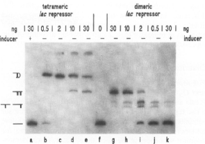
Figure 12: The number of repressors per operon increases with the fold-increase in repressor level relative to the wild-type repressor level. (a) The model prediction calculated from (33) assuming $\chi=0$ and $\alpha_{i},\widehat{\alpha}_{i}$ have wild-type values. (b) When DNA fragments with two lac operators are exposed to increasing repressor levels (lanes b–e), the concentration of binary non-looped fragments increases progressively (Oehler et al., 1990, Fig. 4). The symbols on the left show the structures of the fragments (unary looped at the top, followed by binary non-looped, unary non-looped, and free fragments).

It is therefore clear that in repressor-overexpressed cells, binary and ternary operons are dominant in the absence of the inducer. We expect that they will remain dominant at sufficiently small inducer concentrations. This becomes evident if we plot the fractions of various states of the operon as a function of the inducer concentration. The fractions of non-looped and looped operons containing $i$ repressors are given by

$$\theta_{i}(\chi) \equiv\frac{\phi_{i}(\chi)}{1+\phi_{1}(\chi)+\widehat{\phi}_{1}(\chi)+\phi_{2}(\chi)+\widehat{\phi}_{2}(\chi)+\phi_{3}(\chi)},$$ (48)

$$\widehat{\theta}_{i}(\chi) \equiv\frac{\widehat{\phi}_{i}(\chi)}{1+\phi_{1}(\chi)+\widehat{\phi}_{1}(\chi)+\phi_{2}(\chi)+\widehat{\phi}_{2}(\chi)+\phi_{3}(\chi)}.$$ (49)

The fraction of free operons, which is precisely $\nu$, is given by (38). In wild-type cells, the fraction of binary and ternary operons, ($\theta_{2}+\widehat{\theta}_{2}+\theta_{3}$), is small at all inducer concentrations (Fig 13a, black curve). In repressor-overexpressed cells with 90-fold overexpression, this fraction is dominant for all $\chi\lesssim 5$ (Fig 13b, black curve). If we plot the individual components, $\theta_{2},\widehat{\theta}_{2},\theta_{3}$, of this fraction, it becomes clear that the ternary and binary looped operons are dominant for $\chi\lesssim 3$ (Fig 13c). It follows that the kinetics of repressor-overexpressed cells cannot be captured by eq. (45) — it is necessary to use the more general expression (35).

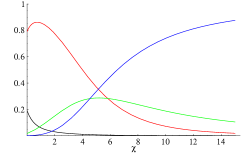
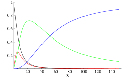
Figure 13: Distribution of the fractions of various states as a function of the inducer concentration: (a) Wild-type cells. (b,c) Repressor-overpressed cells with 90-fold overexpression. In (a, b), the black curve represents the fraction of binary and ternary operons; the red, green, and blue curves represent the fractions of looped unary, non-looped unary, and free operons, respectively. In (c), the full, dashed, and long-dashed lines denote the fractions of ternary, looped binary, and non-looped binary operons, respectively.

We tested the validity of the model by determining the extent to which it could fit the induction curves for cells containing wild-type repressor levels (Fig. 11). The fits do not prove the validity of the model because these induction curves show the variation of only one of the model variables — the fraction of free operons — as a function of the inducer concentration, . If the model is truly valid, the fraction of every looped and non-looped species will vary in a manner consistent with the model. It is therefore particularly useful that these fractions follow simple scaling relations, which are experimentally testable because each fraction migrates at a different speed in polyacrylamide gel electrophoresis (Fig. 12b). To see this, note that there are three distinct trends in Figs. 13b,c: (a) The fraction of free operons increases monotonically, (b) the fractions of ternary and looped binary operons decrease monotonically, and (c) the fractions of the remaining three states of the operon pass through a maximum. These trends follow immediately from the definitions (48)–(49). They are similar to the concentration profiles observed in series reactions ($A\rightarrow B\rightarrow\cdots$), wherein as time progresses, the concentration of the first (resp., last) component decreases (resp., increases) monotonically, and the concentrations of the intermediate components pass through a maximum. In Figs. 13b,c, the inducer concentration plays a role analogous to time: As $\chi$ increases, the ternary operons are successively converted to binary, unary, and free operons. But there is an important difference. Since $\widehat{\phi}_{2}$ and $\phi_{3}$ decrease with $\chi$ at the same rate, the model predicts that the ratio, $\widehat{\theta}_{2}/\theta_{3}$, has the same value, $\widehat{\alpha}_{2}/\alpha_{3}$, at all inducer concentrations. Similarly, the ratio, $\widehat{\theta}_{1}/\theta_{2}$, must have the same value, $\widehat{\alpha}_{1}/\alpha_{2}$, at all inducer concentrations. These scaling relations were obtained by varying the inducer concentrations at fixed repressor levels. If the repressor levels are changed at fixed inducer levels, say, $\chi=0$ (Fig. 12b), the model predicts that $\widehat{\theta}_{i}/\theta_{i}$ will have the same value, $\widehat{\alpha}_{i}/\alpha_{i}$, at all repressor levels. Experimental tests of these scaling relations provide a stringent test of the model. Furthermore, deviations from these scaling relations may reveal the untenable assumptions of the model.

4 Discussion

Given the above results, we can state the conditions under which the kinetics of lac induction can be described by eqs. (1) and (2) of the Yagil & Yagil model. If DNA looping is weak or absent, both equations provide good approximations to the kinetics, but (1) is valid at all inducer concentrations, whereas (2) captures the kinetics only at sufficiently large inducer concentrations. Indeed, the latter equation predicts that the slope of the induction curve is zero at small inducer concentrations. This is inconsistent with the data — the induction curve increases linearly at inducer concentrations as low as $\sim$0.5 $\mu$M, regardless of the presence or absence of DNA looping (Fig. 14).

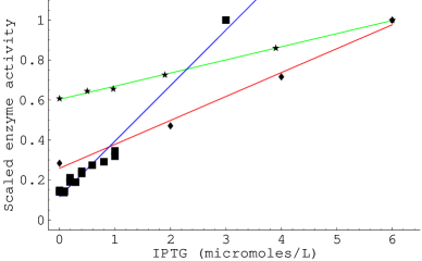
Figure 14: The induction rate increases linearly at small inducer concentrations (Gilbert and Müller-Hill, 1966; Oehler et al., 2006; Overath, 1968). The data corresponds to E. coli BMH8117 $\lambda$Ewt100 ($\blacklozenge$), which contains only the main operator, and E. coli 15TAU lac${}_{2}^{-}$ ($\bigstar$), W3102 ($\blacksquare$) which contain all three operators.

In the presence of DNA looping, the kinetics of wild-type cells are more cooperative than the kinetics predicted by the Yagil & Yagil model, and this cooperativity becomes even more pronounced in repressor-overexpressed cells. This result has important implications for the dynamics of the lac operon. As we show below, it suggests that repressor overexpression can be used to induce bistability in systems that are otherwise bistable.

Molecular biologists have known for a long time that cooperativity plays a central role in genetic switches (Ptashne, 1992, p. 28). This was conclusively demonstrated by recent experiments with the lac operon. Ozbudak et al inserted into the chromosome of E. coli MG 1655 a single copy of a lac reporter gene coding for green fluorescence protein. In these cells, the green fluorescence intensity provides a measure of the instantaneous activity of the lac enzymes. They showed that when these cells were grown exponentially on a medium containing succinate and the gratuitous inducer, TMG, the enzyme activities displayed bistability. Futhermore, this bistability could be captured by the steady states of the equation

$$\frac{de}{dt}=\frac{1+K_{x}^{2}x^{2}}{\alpha_{1}+1+K_{x}^{2}x^{2}}-r_{g}e,\;x\propto e\frac{s}{K_{s}+s}$$

where $e$ and $s$ denote the lac permease activity and extracellular TMG concentration, respectively; $r_{g}$ denotes the specific growth rate on succinate; and the inducer concentration, $x$, is assumed to be proportional to the TMG uptake rate. Bistability occurs precisely because the induction rate, which increases as $e^{2}$, is more cooperative than the dilution rate, which is proportional to $e$ (Fig. 15a, black curves). Indeed, if the repressor level is decreased by “titrating” the repressor with the lac operator, the induction curve loses its cooperativity — it becomes hyperbolic (Fig. 15a, red curve), and the bistability disappears.

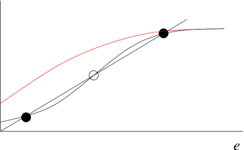
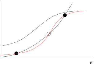
Figure 15: Induction of bistability by repressor overexpression. (a) In wild-type E. coli, there is bistability during growth on succinate + TMG (black curves). If the repressor levels are reduced, the induction rate becomes hyperbolic (red curve), and bistability disappears. (b) In wild-type E. coli, there is no bistability during growth on lactose (black curves). If the repressor is overexpressed, bistability is induced because the induction rate becomes more cooperative (red curve).

The above example shows that bistability can be abolished by decreasing the repressor level, and hence, the cooperativity of the induction curve. It is therefore conceivable that bistability can be imposed upon monostable systems by increasing the repressor level. Ozbudak et al observed that their system exhibited no bistability if the cells were grown on lactose, rather than succinate + TMG (Ozbudak et al., 2004). One hypothesis for explaining the absence of bistability is as follows (Narang and Pilyugin, 2006). During growth on succinate + TMG, the specific growth rate is independent of the lac permease activity. In sharp contrast, during growth on lactose, the specific growth rate is proportional to the specific lactose uptake rate, i.e., $r_{g}\propto es/(K_{s}+s)$, where $s$ now represents the concentration of extracellular lactose. The dilution rate is therefore as cooperative as the induction rate (both rates increase as $e^{2}$), and bistability is impossible (Fig. 15b, black curves). In such systems, bistability can be induced by overexpressing the repressor because the induction rate then increases as $e^{4}$ or $e^{6}$, which is significantly more cooperative than the dilution rate (Fig. 15b, red curve). Thus, the increase in cooperativity generated by high repressor levels can be exploited to impose bistability upon systems that otherwise show little propensity for switch-like behavior. This may be useful in synthetic biology, which is concerned, among other things, with the development of genetic switches.

5 Conclusions

We formulated a model for the kinetics of lac induction which takes due account of the tetrameric structure of the repressor, the existence of the auxiliary operators, and the attendant DNA looping. Analysis of the model shows that:

1. In the absence of DNA looping, the kinetics are given by eq. (25), which is formally similar to the Yagil & Yagil model. In the presence of DNA looping, the kinetics are significantly more cooperative.

2. In wild-type cells, no more than one repressor binds to an operon, and the kinetics are given by eq. (44), which depends on powers of $x$ as high as $x^{4}$. The cooperativity increases markedly because the concentration of looped repressor-operator complexes decreases with the inducer concentration at a rate much faster than the corresponding rate for non-looped complexes.

3. If the repressor is overexpressed in wild-type cells, multiple repressors are bound to most of the operons, and the kinetics are given by eq. (32), which depends on powers of $x$ up to $x^{6}$. The cooperativity is enhanced even further because multi-repressor operons are more sensitive to the inducer concentrations than operons with only one repressor.

4. The model provides good fits to the induction curves for 4 different strains of E. coli. We also show that if the model is correct, the relative concentrations of certain looped and non-looped species must remain the same at all inducer (or repressor) concentrations. These scaling relations, which lie at the heart of the model, can be rigorously tested by gel electrophoresis.

These results should be useful in analyzing kinetic data for induction of operons involving DNA looping, and in formulating dynamic models for induction of such operons.

Appendix A Induction kinetics and repression in cells containing mutant dimers

Equations (18)–(19) were derived for cells containing the tetrameric repressor. If the cells contain mutant dimers that can bind to the operator but do not tetramerize, the corresponding equations are

$$\rho\left(1+\chi\right)^{2}+\omega\nu\left[\rho\bar{\alpha}_{1}+2\rho^{2}\bar{\alpha}_{2}+3\rho^{3}\bar{\alpha}_{3}\right] =1,$$ (50)

$$\nu\left[1+\rho\bar{\alpha}_{1}+\rho^{2}\bar{\alpha}_{2}+\rho^{3}\bar{\alpha}_{3}\right] =1.$$ (51)

where $\rho$ now denotes the fraction of free mutant dimers. These equations differ from eqs. (18)–(19) in three ways: (a) The parameters, $\bar{\alpha}_{i}$, satisfy the relations, $\bar{\alpha}_{1}=\alpha_{1}/2$, $\bar{\alpha}_{2}=\alpha_{2}/4$, $\bar{\alpha}_{3}=\alpha_{3}/8$, since the association constants for dimer-operator binding are half of the corresponding association constants for tetramer-operator binding. (b) The first term of eq. (50) depends on $(1+\chi)^{2}$, rather than $(1+\chi)^{4}$, because mutant dimers have only two inducer-binding sites. (c) The terms in square brackets do not depend on the inducer concentrations because inducer-bound mutant dimers cannot bind to the operator. The latter also implies that the transcription rate is proportional to $T=\nu\left(1+\bar{\kappa}_{2}\rho\right),$ $\bar{\kappa}_{2}=\kappa_{2}/2$, provided $d=0$.

The zeroth-order solution is

$$\rho_{0} =\frac{1}{\left(1+\chi\right)^{2}},$$

$$\nu_{0} =\frac{1}{1+\rho_{0}\bar{\alpha}_{1}+\rho_{0}^{2}\bar{\alpha}_{2}+\rho_{0}^{3}\bar{\alpha}_{3}},$$

which implies that

$$T=\frac{1+\bar{\kappa}_{2}/\left(1+\chi\right)^{2}}{1+\bar{\alpha}_{1}/\left(1+\chi\right)^{2}+\bar{\alpha}_{2}/\left(1+\chi\right)^{4}+\bar{\alpha}_{3}/\left(1+\chi\right)^{6}}.$$

Although these kinetics can be highly cooperative, the parameter values for cells containing wild-type repressor levels are such that the corresponding kinetics are formally similar to eq. (28). Fig. 5b shows that this equation provides a good fit to the induction curve of cells containing mutant dimers.

Figure 16: The model predicts the repression in cells containing mutant dimers (data from Oehler et al., 1990, Table I, and Oehler et al., 1994, Figs 4–5). The full lines show the model predictions, calculated from eqs. (52)–(55) with the wild-type parameter values, $\kappa_{1}=30$, $\kappa_{2}=0.38$, $\kappa_{3}=0.24$, determined in Section 3.

To see this, observe that the values of $\alpha_{1}$, $\alpha_{2}$, $\alpha_{3}$ for cells containing wild-type levels of tetrameric repressor imply that $\bar{\alpha}_{1}=15.5$, $\bar{\alpha}_{2}=5$, $\bar{\alpha}_{3}=0.25$. Since $\bar{\alpha}_{2},\bar{\alpha}_{3}$ are small compared to $\bar{\alpha}_{1}$,

$$\frac{\bar{\alpha}_{2}}{\left(1+\chi\right)^{4}},\frac{\bar{\alpha}_{3}}{\left(1+\chi\right)^{6}}\ll\frac{\bar{\alpha}_{1}}{\left(1+\chi\right)^{2}}$$

for all but a negligibly small range of inducer concentrations. The induction kinetics are therefore formally identical to eq. (28).

The repression in cells containing all three operators is

$$\mathcal{R}_{312}=\frac{1+\bar{\alpha}_{1}+\bar{\alpha}_{2}+\bar{\alpha}_{3}}{1+\bar{\kappa}_{2}},$$ (52)

which implies that

$$\mathcal{R}_{1} =1+\bar{\kappa}_{1}, \mathcal{R}_{2} =1,$$ (53)

$$\mathcal{R}_{3} =1+\bar{\kappa}_{3}, \mathcal{R}_{12} =\frac{1+\bar{\kappa}_{1}+\bar{\kappa}_{2}+\bar{\kappa}_{1}\bar{\kappa}_{2}}{1+\bar{\kappa}_{2}},$$ (54)

$$\mathcal{R}_{32} =\frac{1+\bar{\kappa}_{2}+\bar{\kappa}_{3}+\bar{\kappa}_{2}\bar{\kappa}_{3}}{1+\bar{\kappa}_{2}}, \mathcal{R}_{31} =1+\bar{\kappa}_{1}+\bar{\kappa}_{3}+\bar{\kappa}_{1}\bar{\kappa}_{3},$$ (55)

where $\bar{\kappa}_{i}=\kappa_{i}/2$. Fig. 16 shows the repression predicted by these expressions, assuming that $\kappa_{1},\kappa_{2},\kappa_{3}$ have the values estimated in Section 3 from the data for cells containing the tetrameric repressor. The good agreement with the repression data for cells containing mutant dimers suggests that the model and the parameter values are plausible.

Appendix B Solution of eqs. (18)–(19) by regular perturbation

We wish to solve the equations

$$\rho\left(1+\chi\right)^{4}+\omega\nu(\rho f_{1}+2\rho^{2}f_{2}+3\rho^{3}f_{3}) =1,$$ (56)

$$\nu(1+\rho f_{1}+\rho^{2}f_{2}+\rho^{3}f_{3}) =1,$$ (57)

for small $\omega$. To this end, assume that the solutions have the form

$$\rho =\rho_{0}+\omega\rho_{1}+O(\omega^{2}),$$ (58)

$$\nu =\nu_{0}+\omega\nu_{1}+O(\omega^{2}).$$ (59)

Substituting these solutions in (56)–(57), and collecting terms with like powers of $\omega$ yields

$$\left[\rho_{0}\left(1+\chi\right)^{4}-1\right]+\omega\left[\rho_{1}\left(1+\chi\right)^{4}+\nu_{0}\left(\rho_{0}f_{1}+2\rho_{0}^{2}f_{2}+3\rho_{0}^{3}f_{3}\right)\right]+\ldots =0,$$

$$\left[\nu_{0}\left(1+\rho_{0}f_{1}+\rho_{0}^{2}f_{2}+\rho_{0}^{3}f_{3}\right)-1\right]+\omega\left[\nu_{0}\rho_{1}\left(f_{1}+2\rho_{0}f_{2}+3\rho_{0}^{2}f_{3}\right)+\right.$$

$$+\left.\nu_{1}\left(1+\rho_{0}f_{1}+\rho_{0}^{2}f_{2}+\rho_{0}^{3}f_{3}\right)\right]+\ldots =0.$$

It follows that

$$\rho_{0} =\frac{1}{\left(1+\chi\right)^{4}},$$

$$\nu_{0} =\frac{1}{1+\rho_{0}f_{1}+\rho_{0}^{2}f_{2}+\rho_{0}^{3}f_{3}},$$

$$\rho_{1} =-\frac{\nu_{0}}{\left(1+\chi\right)^{4}}\left(\rho_{0}f_{1}+2\rho_{0}^{2}f_{2}+3\rho_{0}^{3}f_{3}\right),$$

$$\nu_{1} =-\nu_{0}\rho_{1}\frac{f_{1}+2\rho_{0}f_{2}+3\rho_{0}^{2}f_{3}}{1+\rho_{0}f_{1}+\rho_{0}^{2}f_{2}+\rho_{0}^{3}f_{3}}.$$

If we define

$$\Omega_{0}\equiv\frac{\rho_{0}f_{1}+2\rho_{0}^{2}f_{2}+3\rho_{0}^{2}f_{3}}{1+\rho_{0}f_{1}+\rho_{0}^{2}f_{2}+\rho_{0}^{3}f_{3}},$$ (60)

$\rho_{1}$ and $\nu_{1}$ can be written as

$$\rho_{1}=-\rho_{0}\Omega_{0},\;\nu_{1}=\nu_{0}\Omega_{0}^{2}.$$

Substituting these expressions in (58)–(59) yields

$$\rho =\rho_{0}\left(1-\omega\Omega_{0}\right)+O(\omega^{2}),$$ (61)

$$\nu =\nu_{0}\left(1+\omega\Omega_{0}^{2}\right)+O(\omega^{2}).$$ (62)

These are the first-order solutions for the general model.

The parameter $\Omega_{0}$ approximates the average number of repressors bound to an operon because (60) can be rewritten as

$$\Omega_{0}=\theta_{1,t}+2\theta_{2,t}+3\theta_{3,t},$$

where

$$\theta_{i,t}\equiv\frac{\rho_{0}^{i}f_{i}}{1+\rho_{0}f_{1}+\rho_{0}^{2}f_{2}+\rho_{0}^{3}f_{3}},\;i=1,2,3.$$

is the fraction of operons containing $i$ repressors. It follows that $\Omega_{0}$ must lie between 0 and 3. In the absence of the inducer, $\Omega_{0}$ increases with repressor overexpression from $\sim$1 to 3 (Fig. 12). However, the relative error for $\nu_{0}$ does not exceed $\sim$20% (Fig. 17).

Figure 17: The relative error for $\nu_{0}$ does not exceed $\sim$20%. The relative error was calculated assuming $\chi=0$, $\omega=0.2$, and $\alpha_{i},\widehat{\alpha}_{i}$ have wild-type values.

In the absence of the auxiliary operators, $f_{2}=f_{3}=0$. In this case

$$\nu_{0}=\frac{1}{1+\rho_{0}f_{1}},\;\Omega_{0}=\frac{\rho_{0}f_{1}}{1+\rho_{0}f_{1}}\Rightarrow\Omega_{0}=1-\nu_{0}.$$

Substituting this relation in (61)–(62) yields

$$\rho =\rho_{0}\left[1-\omega\left(1-\nu_{0}\right)\right]+O(\omega^{2}),$$

$$\nu =\nu_{0}\left[1+\omega\left(1-\nu_{0}\right)^{2}\right]+O(\omega^{2}).$$

References

- Ackers et al. (1982) Ackers, G. K., Johnson, A. D., Shea, M. A., Feb 1982. Quantitative model for gene regulation by lambda phage repressor. Proc Natl Acad Sci U S A 79 (4), 1129–1133.
- Barry and Matthews (1999) Barry, J. K., Matthews, K. S., May 1999. Thermodynamic analysis of unfolding and dissociation in lactose repressor protein. Biochemistry 38 (20), 6520–6528.
- Carroll et al. (2005) Carroll, S. B., Grenier, J. K., Weatherbee, S. D., 2005. From DNA to Diversity: Molecular Genetics and the Evolution of Animal Design, 2nd Edition. Blackwell Publishing.
- Chung and Stephanopoulos (1996) Chung, J. D., Stephanopoulos, G., 1996. On physiological multiplicity and population heterogeneity of biological systems. Chem. Eng. Sc. 51, 1509–1521.
- Gilbert and Müller-Hill (1966) Gilbert, W., Müller-Hill, B., Dec 1966. Isolation of the lac repressor. Proc Natl Acad Sci U S A 56 (6), 1891–1898.
- Herzenberg (1959) Herzenberg, L. A., Feb 1959. Studies on the induction of -galactosidase in a cryptic strain of Escherichia coli. Biochim Biophys Acta 31 (2), 525–538.
- Laurent et al. (2005) Laurent, M., Charvin, G., Guespin-Michel, J., Dec 2005. Bistability and hysteresis in epigenetic regulation of the lactose operon. Since Delbrück, a long series of ignored models. Cell Mol Biol (Noisy-le-grand) 51 (7), 583–594.
- Lewis (2005) Lewis, M., Jun 2005. The lac repressor. C R Biol 328 (6), 521–548.
- Müller-Hill (1996) Müller-Hill, B., 1996. The lac operon, 1st Edition. de Gruyter, Berlin.
- Narang and Pilyugin (2006) Narang, A., Pilyugin, S. S., December 2006. Why does the lac exhibit no bistability during growth of Escherichia coli on lactose or lactose + glucose?, submitted, Bull. Math. Biol.
- Oehler et al. (2006) Oehler, S., Alberti, S., Müller-Hill, B., 2006. Induction of the lac promoter in the absence of DNA loops and the stoichiometry of induction. Nucleic Acids Res 34 (2), 606–612.
- Oehler et al. (1994) Oehler, S., Amouyal, M., Kolkhof, P., von Wilcken-Bergmann, B., Müller-Hill, B., Jul 1994. Quality and position of the three lac operators of E. coli define efficiency of repression. EMBO J 13 (14), 3348–3355.
- Oehler et al. (1990) Oehler, S., Eismann, E. R., Krämer, H., Müller-Hill, B., Apr 1990. The three operators of the lac operon cooperate in repression. EMBO J 9 (4), 973–979.
- Overath (1968) Overath, P., 1968. Control of basal level activity of -galactosidase in Escherichia coli. Mol Gen Genet 101 (2), 155–165.
- Ozbudak et al. (2004) Ozbudak, E. M., Thattai, M., Lim, H. N., Shraiman, B. I., van Oudenaarden, A., 2004. Multistability in the lactose utilization network of Escherichia coli. Nature 427, 737–740.
- Ptashne (1992) Ptashne, M., 1992. A Genetic Switch: Phage and Higher Organisms, 2nd Edition. Cell Press & Blackwell Scientific Publications, Cambridge, MA.
- Ptashne and Gann (2002) Ptashne, M., Gann, A., 2002. Genes & Signals. Cold Spring Harbor Laboratory Press, Cold Spring Harbor, New York.
- Vilar and Leibler (2003) Vilar, J. M. G., Leibler, S., Aug 2003. DNA looping and physical constraints on transcription regulation. J Mol Biol 331 (5), 981–989.
- Yagil and Yagil (1971) Yagil, G., Yagil, E., 1971. On the relation between effector concentration and the rate of induced enzyme synthesis. Biophys. J. 11, 11–17.