Species clustering in competitive Lotka-Volterra models

Abstract

We study the properties of Lotka-Volterra competitive models in which the intensity of the interaction among species depends on their position along an abstract niche space through a competition kernel. We show analytically and numerically that the properties of these models change dramatically when the Fourier transform of this kernel is not positive definite, due to a pattern forming instability. We estimate properties of the species distributions, such as the steady number of species and their spacings, for different types of kernels.

It is widely believed that competition among species greatly influences global features of ecosystems. One of the most relevant is the fact that ecosystems can host a limited number of species. The common explanation is the so-called limiting similarity macarthurlevins and involves representing species as points in an abstract niche space, whose coordinates quantify the phenotypic traits of a species which are relevant for the consumption of resources, usually the typical size of individuals, but also preferred prey, optimal temperature and so on. On general grounds, one expects that a species experiences a stronger competition with the closer species in this space. As a consequence, a species can survive if it is able to maintain its distance with the others above a minimum value which depends on the intensity of competition. On the contrary, when the distance between two species becomes too small, the unavoidable difference in how efficiently the two species feed on the resources will make one of the two outcompete the other, that will go extinct: this is the essence of the competitive exclusion principle hardin , and it can be thought as the theoretical grounding of the concept of ecological niche. Thus, one expects a stable ecosystem to display a finite number of species, more or less equidistant in the niche space. The finiteness of the number of species has been observed in several competition models szabo and, recently, it has been rigorously demonstrated for a general class of them gyllenberg .

Deviations from the above scenario have aroused renewed interest recently, when it was observed numerically schefferpnas that the equilibrium state of rather standard models is not always characterized by a homogeneous distribution of species in niche space. Instead, clumpy distributions, with clusters of many species separated by unoccupied regions, are observed. Evidences of a similar phenomenon have been observed recently in an evolutionary model brigatti , suggesting that a theoretical explanation of these patterns could bring new insights in the study of speciation mechanisms johansson .

In this Letter, we study the Lotka-Volterra (LV) competitive model as the prototype of competitive systems. While the statistical properties of the antisymmetric LV model have been addressed recently tokitaprl , not much has been demonstrated about the statistics of the competitive case. Through this paper we will use the language of ecological species competition, but we stress that the LV set of equations appears in contexts as diverse as multimode dynamics in optical systems optics , technology substitution tech , or mode interaction in crystallization fronts Kurtze , and it is the natural starting point when modelling competitive systems. Our main result is that the macroscopic clustering of species is related to a pattern forming transition that separates two different qualitative behaviors. This is the same phenomenology found in birth-death particle systems with interaction at a distance, in which individuals typically aggregate forming clusters which arrange in an ordered pattern refbugs1 , with the physical space playing the role of niche space. The feature which is relevant for this transition is not the intensity of the competition, but the functional form of the competition kernel. We estimate analytically the number of species in cases at both sides of the transition, and also discuss the role of species heterogeneity.

Mathematically, one has competition when the growth of a species affects negatively the growth rate of other species. One of the simplest implementations of that is the LV competitive model:

$$\dot{n_{i}}=n_{i}\left(r-a_{i}\sum_{j=1}^{N}g(|x_{i}-x_{j}|)n_{j}\right)\ ,\qquad\ i=1\ldots N.$$ (1)

$N$ is the number of species and $n_{i}$ denotes the population of species $i$. Each species is characterized by a growth rate $r$ and a competition parameter $a_{i}$ (we take into account differences among species only in the latter parameter). A species is also characterized by a position $x_{i}$ in a niche space that we assume, for simplicity, to be the segment $[0,L]$ with periodic boundary conditions. Generalization to a multidimensional niche space is straightforward, and we expect the unrealistic boundary conditions assumed here to be irrelevant except close to the interval endpoints. The competition kernel $g(x)$ is a non-negative and non-increasing function. Note that the sum in Eq.(1) contains the self-interaction term $g(0)n_{i}$.

To fully specify the dynamics, we should state how the $x_{i}$ are assigned to species and eventually changed. We consider a slow immigration rate $I$ at which new species, characterized by a random phenotype $x\in[0,L]$, are introduced in the system with a small random population $\delta n$. This choice is appropriate to model a situation like an ecological community on an island macarthurwilson . In addition, we consider extinct, and remove from the system, species whose population goes below a given threshold $n_{T}$. When $I^{-1}$ is very large compared to the timescales of population dynamics, the system has time to relax to a quasisteady state after each immigration event. Our interest here is in the characteristics of these states, in which immigration plays almost no role. An efficient way to obtain them is by running simulations of Eq. (1) with a small amount of immigration, which is then “switched off” after some time. By a choice of the time and the population units, we can set $r=1$ and $n_{T}=1$ (thus the parameters $a_{i}$ are really $a_{i}n_{T}/r$). We also measure all distances in niche space in units of $L$, so that $L=1$.

Figure 1: Steady states of system (1), with $a_{i}=a=0.1$, obtained by evolving a random configuration, initially of $200$ species, for a time $t=5\times 10^{5}$. The immigration rate was initially $I=0.004$, and switched off after half simulation. Top panels: Competition kernel $g_{1}(x)=\exp(-x/R)$ (left), and $g_{4}(x)=\exp[-(x/R)^{4}]$ (right), with $R=0.1$. In the bottom panels, we added a Kronecker delta $\delta_{x0}$ to the kernels above. In the last panel, the dotted line is a steady solution of (2), arbitrarily scaled in the vertical to fit in the same plot.

In Fig. 1 we show numerical results for the dynamics just defined, for $a_{i}=a$ for all $i$. In the top row we compare the distribution of species with kernels $g_{1}(x)=\exp(-x/R)$ and $g_{4}(x)=\exp[-(x/R)^{4}]$. In the exponential case (left) species occupy the full niche space. Although they are not perfectly equispaced and there are differences in the population sizes, there is a clear average interspecies distance, which corresponds to $1/N$. In the quartic-exponential case (right), a much more regular pattern emerges, with different species perfectly equidistant (and all with the same population). Since growth limitation is known to affect species distribution schefferpnas , we plot in the bottom row results for kernels $g_{1}(x)+\delta_{x0}$ and $g_{4}(x)+\delta_{x0}$, i.e. the same kernels but with an enhanced value of the self-competition coefficient $g(0)$. Here the difference is even more striking: the exponential case is similar to the previous one, but the quartic case shows clear clusters of species separated by empty regions.

To understand the origin of the periodic patterns, we write a continuum evolution equation for the field $\phi(x,t)$, the expected density of individuals in a given point $x$ of the niche space as a function of time:

$$\partial_{t}\phi(x,t)=\phi(x,t)\left(1-a\int g(|x-y|)\phi(y,t)dy\right)+s,$$ (2)

which is a mean field version of Eq. (1) for $a_{i}=a$. In this macroscopic description, we neglect fluctuations in the immigration process by using a constant rate $s=I\delta n$. The stationary homogeneous solutions of Eq. (2) are $\phi_{0}=(1\pm\sqrt{1+4s\hat{a}})/(2\hat{a})$, where $\hat{a}=a\mathcal{N}$, with $\mathcal{N}=\int g(x)dx$. Of the two solutions, only the one with the plus sign is acceptable since the other leads to a negative density (this second solution corresponds to the extinct absorbing state when $s=0$). We analyze the stability of the positive solution by considering a small harmonic perturbation $\phi=\phi_{0}+\epsilon\exp(\lambda t+ikx)$. Substituting into (2), the first order in $\epsilon$ gives the following dispersion relation:

$$\lambda(k)=1-\phi_{0}\hat{a}\left(1+\frac{\tilde{g}(k)}{\mathcal{N}}\right)$$ (3)

where $\tilde{g}(k)=\int g(x)\exp(-ikx)dx$ is the Fourier transform of $g(x)$. When $\lambda$ becomes positive for some values of $k$, the constant solution of (2) is unstable, signaling a pattern forming transition CrossHoh with the characteristic length scale of the pattern determined by the value of $k$ at which $\lambda(k)$ is maximum. For Eq. (3), in the limit $s\to 0$, it is a sufficient and necessary condition for instability that the Fourier transform of the kernel, $\tilde{g}$, takes negative values (notice that $\phi_{0}\hat{a}\geq 1$, with $\phi_{0}\hat{a}\sim 1$ in the limit $s\rightarrow 0$; for sufficiently large $s$, the homogeneous state regains stability). To exemplify this mechanism, we consider the family of kernels $g_{\sigma}(x)=\exp[-(x/R)^{\sigma}]$, being $\sigma\geq 0$ and $R$ the typical competition range. It is known giraud that this family of functions has non-negative Fourier transform for $0\leq\sigma\leq 2$. Interestingly enough, the Gaussian kernel, which is the commonly adopted one macarthurlevins ; schefferpnas , corresponds to the marginal case. This may imply that some results previously obtained for this case could be non robust and largely affected by the way immigration is introduced, the presence or absence of diffusion processes in niche space, etc.

We quantify the pattern-forming transition in terms of the structure function, $S(k)=|\sum_{j}n_{j}\exp(ikx_{j})|^{2}$, of the stationary distribution of species obtained from the simulations. The position and height of its maximum identify periodic structures. In Fig. 2 we plot (left panel) the maximum height of $S$ as a function of the exponent $\sigma$ of the kernel. The sharp increase of $\max S$ for $\sigma>2$ indicates the formation of periodic structures in this range. This is confirmed by the right panel plot, where we show the position $k_{m}$ of the peak of $S$, together with the value $k_{L}$ at which the linear growth, expression (3), has a maximum. Note that the location of this maximum is independent of the parameters $a$ and $s$, being only dependent on the parameters in $g_{\sigma}(x)$ ($R$ and $\sigma$; the dependence on $R$ disappears when considering $k_{L}R$). The striking agreement between $k_{m}$ and $k_{L}$ for $\sigma>2$ confirms that the linear pattern forming instability of the homogeneous distribution is the mechanism responsible for the periodic species arrangement observed in that range. Except when $\sigma\approx 2$, the value of $k_{L}R$ is in the range 4.5-5.0, so that the pattern periodicity would be $d\approx 2\pi/k_{L}\approx\alpha R$, with $\alpha\approx 1.3-1.4$, as observed in Fig. 1 (right panels).

Another difference between $\sigma\leq 2$ and $\sigma>2$, visible in Fig. 1, is the existence in the later case of exclusion zones around established species, in which immigrants have not been able to settle. We can understand the presence of these regions also from the density equation (2), for $s=0$, by noticing that its steady stable solutions $\phi_{st}(x)$ necessarily have regions with $\phi_{st}(x)=0$ in the pattern forming case. This can be seen from the steady state condition $\int dyg(|x-y|)\phi_{st}(y)=1/a$, which is valid at all niche locations $x$ at which $\phi_{st}(x)\neq 0$. If these locations cover in fact the full niche space $[0,1]$, we can solve the steady state condition by Fourier transform and find that the only solution (for nonconstant $g(x)$) is the homogeneous one $\phi_{st}(x)=(a{\mathcal{N}})^{-1}$. Since we know that this is linearly unstable when the Fourier transform of $g(x)$ is not positive definite, we conclude that steady stable solutions of (2) in the pattern forming case must have regions of zero density, which we identify with the exclusion zones. Given the absorbing character of the $\phi=0$ state, many steady solutions exist, differing in the amount and location of the $\phi_{st}=0$ segments, but the most relevant are the ones attained when $s\to 0^{+}$. Figure 1 (bottom right) shows one of these solutions, numerically obtained (for a kernel $g_{4}(x)+\delta(x)$). The steady solution corresponding to the $g_{4}(x)$ kernel of the top right panel is zero everywhere except at a set of periodically spaced delta functions. In both cases the discrete species distribution is well represented by the solutions of (2).

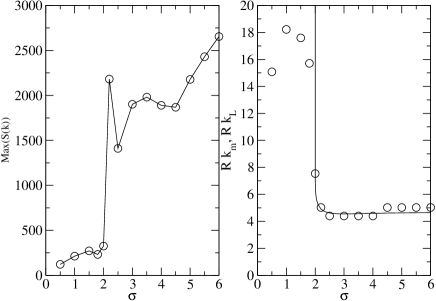
Figure 2: Left panel: maximum of $\left<S(k)\right>$, the structure function averaged over 1000 realizations of stationary distributions of species (obtained after a time $t=10^{5}$, without immigration during the last half of it) as a function of $\sigma$, for $R=0.1$, $a=0.1$. Right panel: position of the peak $k_{m}$ vs $\sigma$ (circles), together with the linearly fastest growing mode $k_{L}$ (line), from (3). For $\sigma>2$, the difference between $k_{m}$ and $k_{L}$ is always smaller than the finite-size discretization of the values of $k_{m}$.

When $\tilde{g}(k)$ remains positive, as for $g_{\sigma}(x)$ with $\sigma\leq 2$, $\lambda(k)$ remains negative, and there are no patterns nor exclusion zones surviving in steady solutions of the density equation for $s\to 0^{+}$. Thus, the characteristic distance between species, observed in Figs. 1 and 2 to be qualitatively different from the case $\sigma>2$, should be determined by a different mechanism. We explore it for the exponential kernel, $g_{1}(x)=\exp(-x/R)$, because it allows some analytical estimates. Fig. 3 shows the number of species at equilibrium for $a_{i}=a$, and also in the heterogeneous situation in which the $a_{i}$’s are independent random variables uniformly distributed between $0.95\bar{a}$ and $1.05\bar{a}$, being $\bar{a}$ an average value.

Figure 3: Number of species as a function of competition coefficient $a$ (left panel, $R=0.1$) and the interaction distance $R$ (right panel, $a=0.1$). Symbols joined by dashed and solid lines are for the cases of $a_{i}^{\prime}s$ heterogeneity (for which $\bar{a}$ is plotted instead of $a$), and non-heterogeneity, respectively. The upper dot-dashed lines are from the approximation (4).

During the system evolution (in the non-heterogeneous case) we observe that, when the species are far from the extinction threshold, it is always possible for a new species to successfully settle between two of them. But as a consequence the populations of these neighboring species get reduced. This brings the species populations closer to $n_{T}$ as the number of species increases, and eventually no new species will be admitted. Thus, in this $\sigma<2$ case, the mechanism fixing a maximum number of species, and thus a characteristic mean distance $d$ among them, is the presence of the extinction threshold $n_{T}$.

Fig. 3 shows that the number of species $N$ (in the steady state obtained after switching off immigration) grows linearly with $1/R$ and with $1/a$ in the case of equal species, while heterogeneity slows down the increase with $1/R$ and almost stops it with $1/\bar{a}$. Notice that decreasing $a$ is the same as decreasing the threshold value $n_{T}$ due to our rescaling of the equations. We can explain these dependences by considering an ideal steady state made of equidistant species, at distance $d$, and having the same population $n^{*}$. The equilibrium condition for the system of equations (1) in the exponential kernel case becomes $\tanh(d/2R)=an^{*}$, which gives $d\approx 2aRn^{*}$ in the limit $(d/2R)\ll 1$. Recalling that $N=1/d$, each population $n^{*}$ decreases as the number of species increases during immigration. The limit, setting the steady state, will be the situation in which $n^{*}=n_{T}=1$, for which no new immigrant can be accepted. Thus we estimate the equilibrium number of species in this case as

$$N\approx\left(2aR\right)^{-1}.$$ (4)

This is only a rough approximation, since species are not equidistant nor equipopulated in the true equilibrium, but provides an explanation for the observed linear scaling of $N$ with $1/a$ and $1/R$. Fig. 3 shows that it gives an upper estimation for the number of species in the less ordered distributions actually found.

The case with heterogeneity of Fig. 3 shows a clearly different mechanism: the number of species does not change with $\bar{a}$ and consequently with $n_{T}$. Thus, this scenario is qualitatively similar to the pattern forming case: there is a distance in the niche space, not related to the threshold value, of the order of the interaction range. Two species cannot survive due to heterogeneity if they are closer than this distance, independently on the mean competition strength.

To clarify this mechanism, we consider the role of heterogeneity in the long-range case of a constant kernel, $g(x)=1$ for all $x$. This may be interpreted as a case in which the kernel decaying distance goes to infinity. Summing all the equations in (1) we obtain an equation for the total population $N_{tot}=\sum_{j}n_{j}$:

$$\dot{N}_{tot}=N_{tot}(1-\langle a\rangle N_{tot})$$ (5)

where $\langle a\rangle=(\sum_{j}a_{j}n_{j})/N_{tot}$. After a short time, the equilibrium value $N_{tot}=\langle a\rangle^{-1}$ would be attained and we can plug this value back into Eqs. (1) to obtain $\dot{n}_{i}=n_{i}(1-a_{i}/\langle a\rangle)$, valid at longer times. In the case of equal species, one has $a_{i}=\bar{a}=\langle a\rangle$ and all possible states with $a\sum_{j}n_{j}=1$ are allowed. In the heterogeneous case, species having $a_{i}<\langle a\rangle$ will grow while the others will decrease their population and finally go extinct. Meanwhile, it is easy to realize that $\langle a\rangle$ will increase, sending more and more species below the extinction threshold. The final result, valid for any initial distribution of the $a_{i}$’s, is that just one species will survive, as confirmed by simulations (not shown).

To conclude, we studied analytically and numerically the collective behavior of competitive Lotka-Volterra systems. Our main message is that the form of the competition kernel changes drastically the equilibrium distribution of species. Species clustering with periodic spacings of the order of the interaction range can occur at one side of a pattern forming transition, whereas smaller spacings, depending on the interaction strength $a$, occur at the other. Surprisingly, the Gaussian kernel, the one usually considered in the literature, corresponds to a frontier case. Diversity has been shown to alter qualitatively the competition outcome. Generalization to the case of a multidimensional niche space is straightforward and does not change qualitatively our results. Diffusion in niche space, modelling mutations schefferpnas , can be introduced and has a stabilizing effect somehow similar to that of the immigration rate $s$.

- (1) R. MacArthur and R. Levins, Am. Nat. 101, 377 (1967).
- (2) G. Hardin, Science 131, 1292 (1960).
- (3) P. Szabó and G. Meszéna, Oikos 112, 612 (2006).
- (4) M. Gyllenberg and G. Meszéna, J. Math. Biol. 50, 133 (2005).
- (5) M. Scheffer and E.H. Van Nes, Proc. Natl. Ac. Sci. 103(16), 6230 (2006).
- (6) E. Brigatti, J.S.S. Martins and I. Roditi, Physica A, in press.
- (7) J. Johansson and J. Ripa, Am. Nat. 168, 572 (2006).
- (8) K. Tokita, Phys. Rev. Lett. 93, 178102 (2004).
- (9) C. Benkert and D.Z. Anderson, Phys. Rev. A 44, 4633 (1991).
- (10) C.W.I. Pistorius and J.M. Utterback, Res. Policy 26, 67 (1997).
- (11) D.A. Kurtze, Phys. Rev. B 40, 11104 (1989).
- (12) E. Hernández-García and C. López, Phys. Rev. E 70 016216 (2004); C. López and E. Hernández-García, Physica D 199, 223 (2004).
- (13) R. MacArthur and E. Wilson, The theory of island biogeography, Princeton University Press (1967); S.P. Hubbell The Unified Neutral Theory of Biodiversity and Biogeography, Princeton University Press (2001); I. Volkov, J.R. Banavar, S.P. Hubbell, A. Maritan, Nature 424(6952), 1035 (2003); S. Pigolotti, A. Flammini, A. Maritan, Phys. Rev. E 70, 011916 (2004).
- (14) M.C. Cross and P.C. Hohenberg, Rev. Mod. Phys. 65, 851 (1993).
- (15) B.G. Giraud, Acta Phys. Polon. B 37, 331 (2006).