Finding Sequence Features in Tissue-specific Sequences

Abstract

The discovery of motifs underlying gene expression is a challenging one. Some of these motifs are known transcription factors, but sequence inspection often provides valuable clues, even discovery of novel motifs with uncharacterized function in gene expression. Coupled with the complexity underlying tissue-specific gene expression, there are several motifs that are putatively responsible for expression in a certain cell type. This has important implications in understanding fundamental biological processes, such as development and disease progression. In this work, we present an approach to the principled selection of motifs (not necessarily transcription factor sites) and examine its application to several questions in current bioinformatics research.

There are two main contributions of this work: Firstly, we introduce a new metric for variable selection during classification , and secondly, we investigate a problem of finding specific sequence motifs that underlie tissue specific gene expression. In conjunction with the SVM classifier we find these motifs and discover several novel motifs which have not yet been attributed with any particular functional role (eg: TFBS binding motifs). We hypothesize that the discovery of these motifs would enable the large-scale investigation for the tissue specific regulatory potential of any conserved sequence element identified from genome-wide studies.

Finally, we propose the utility of this developed framework to not only aid discovery of discriminatory motifs, but also to examine the role of any motif of choice in co-regulation or co-expression of gene groups.

I Introduction

Understanding the mechanisms underlying regulation of tissue specific gene expression is still a challenging question that does not have a satisfactory explanation. While all mature cells in the body have a complete copy of the human genome, each cell type only expresses those genes it needs to carry out its assigned task. This includes genes required for basic cellular maintenance (often called ”house keeping genes”) and those genes whose function is specific to the particular tissue type the cell belongs to. Gene expression by way of transcription is the process of generation of messenger RNA (mRNA) from the DNA template representing the gene. It is the intermediate step before the generation of functional protein from messenger RNA. During gene expression (Fig. 1), transcription factor proteins are recruited at the proximal promoter of the gene as well as at sequence elements (enhancers/silencers) which can lie several hundreds of kilobases from the gene’s transcriptional start site.

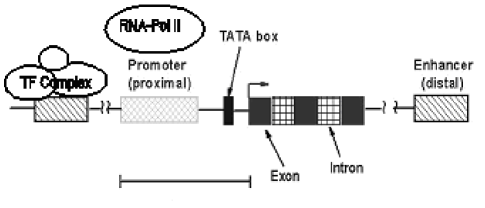
Figure 1: Schematic of Transcriptional Regulation.

The combination of the basal transcriptional machinery at the promoter coupled with the transcription factor complexes at the distal regulatory elements are collectively involved in directing tissue specific expression of genes. Some of the common features of these distal regulatory elements are:

• Non-coding elements: Distal regulatory elements are non-coding and can eitehr be intronic or intergenic region on the genome. Hence previous models of gene finding are not applicable herein. Moreover, with over 98% of the annotated genome being non-coding the precise localization of regulatory elements that underlie tissue-specific gene expression is a challenging problem.

• Distance/orientation independent: An enhancer can act from great genomic distances (hundreds of kilobases) to regulate gene expression in conjunction with the proximal promoter, possibly via a looping mechanism. They can lie upstream or downstream of the actual gene.

• Promoter dependent: Since the action at a distance of these elements involves the recruitment of transcription factors that direct tissue-specific gene expression, the promoter that they interact with is critical.

Though there are instances where a gene harbors tissue specific activity at their promoter itself, there is considerable interest to examine the long range elements (LREs) for a detailed understanding of their regulatory role in gene expression during biological processes like organ development and disease progression [39]. An in-silico examination of the sequence properties of such LREs would result in computational strategies to find novel LREs genomewide that govern tissue specific expression for any gene of interest.

Our primary question in this regard is: are there any discriminating sequence properties of such LRE elements that determine tissue specific gene expression - more particularly, are there any sequence motifs in such regulatory elements that can aid discovery of new elements with similar potential for tissue-specific regulation genomewide [22]. We remind the reader that a similar approach was used in gene finding algorithms, wherein sequence features of exons are examined to facilitate the discovery of novel genes. In popular gene finding algorithms [21], discriminatory motifs are identified from annotated genes and non-coding regions. Such an approach can be extended to this situation too wherein we look for motifs discriminating regulatory and neutral non-coding elements. In this work, we explore the possible existence of such discriminating sequence motifs in two kinds of biologically relevant regulatory sequences:

• Promoters of tissue specific genes: Before the widespread discovery of long-range regulatory elements (LREs) it was hypothesized that promoters governed gene expression entirely. There is substantial evidence for the binding of tissue-specific transcription factors at the promoters of expressed genes. This suggests that, in spite of newer information implicating the role of LREs, promoters might also have interesting motifs that govern tissue-specific expression, that are potentially relevant to the discovery of new LREs de-novo.

  Another practical reason for the examination of promoters is that their locations (and genomic sequences) are more unambiguously delineated on genome databases (like UCSC or Ensembl). Sufficient data (http://symatlas.gnf.org) on the expression of genes is publicly available for analysis.

  We set up the motif discovery as a feature extraction problem from these tissue-specific promoter sequences and then build a support vector machine (SVM) classifier to classify new promoters into specific and non-specific categories based on the identified sequence features (motifs). Using the SVM classifier algorithm we are able to accurately classify 70% of tissue specific genes based upon their upstream promoter region sequences alone.

• Known long range regulatory elements (LRE) motifs: To analyze the motifs in LRE elements, there is a need for an experimental dataset of elements that confer tissue-specific expression in some eukaryotic animal model. For our purpose, we examine the results of this approach on other new data source of interest - the Enhancer Browser at http://enhancer.lbl.gov which has results of expression of ultraconserved genome elements in transgenic mice [23]. An examination of these ultraconserved enhancers is useful for the extraction of discriminatory motifs to distinguish these regulatory elements from non-regulatory (neutral) ones. Here the results indicate that upto 90% of the sequences can be correctly classified using these identified motifs.

We note that some of the identified motifs might not be transcription factor binding motifs, and would need to be functionally characterized. This is an advantage of our method - instead of constraining ourselves by the degeneracy present in TF databases (like TRANSFAC/JASPAR), we look for all sequences of a fixed length.

II Contributions

From microarray expression data, ([11],[12]) proposes an approach to assign genes into tissue specific and non-specific types using an entropy criterion. They use the variation in expression and its divergence from ubiquitous expression (uniform distribution across all tissue types) to make this assignment. From this assignment, several features like CpG island density, frequency of transcription factor motif occurrence, can be examined to discriminate these two subgroups. However, a denovo examination of ’every’ sequence feature in sequence and its subsequent interpretation has not been pursued adequately. Other work has explored the existence of key motifs (transcription factor binding sites) in the promoters of tissue-specific genes [25].

For the purpose of identifying discriminative motifs from the training data (tissue-specific promoters or LREs), our approach is two-pronged:

• Variable selection: We first find those sequence motifs that can discriminate between tissue-specific and non-specific elements. In machine learning, this is a feature selection problem. Here, these features are the counts of sequence motifs in these training sequences. Without loss of generality, we can use six-nucleotide motifs (hexamers) as the motif features. This is based on the observation that most transcription factor binding motifs have a 5-6 nucleotide core sequence with degeneracy at the ends of the motif. Another reason is that we need to find a length that captures biologically meaningful information as well as does not lead to an unduly large search space. Even though our motivation for choosing hexamers was independent, a similar setup has been referred to in ([2], [5]). We find that $4^{6}$ possibilities (from hexamer sequences) yields good performance without being unduly costly, computationally. The overall presented approach, however, does not depend of this choice of motif length and can be scaled depending on biological intuition.

  In the first part of the work in this paper, we present a novel feature selection approach (based on a new information theoretic quantity called directed information - DTI) that can be applied to such learning problems.

• Classifier design: After discovering key discriminating motifs from the above DTI step, we proceed to build a SVM classifier that separates the samples between the two classes (specific and non-specific) from this feature space. One distinction we make is that the class label is a perceptual abstraction (based on our intuition and experience). The feature space (hexamer counts) is a physical/measurement space - this is what we can look for.

Apart from the novel feature selection approach, our contributions to bioinformatics methodology are outlined below:

From the identified motifs, we ask several related questions:.

• Are there any common motifs identified from tissue-specific promoters and corresponding enhancers, both underlying expression in the same tissue?. To answer this, we examine brain-specific promoters and enhancers.

• Do these motifs correlate with known motifs (transcription factor binding sites),

• how useful are these motifs in predicting new regulatory elements?.

This work differs from that in ([2], [5]), in several aspects. We present the novel DTI based feature selection procedure as part of an overall unified framework to answer several questions in bioinformatics, not limited to finding discriminating motifs between two classes of sequences. Particularly, one of the advantages of the proposed approach is the examination of any particular motif as a potential discriminator between two classes. Also, this work accounts for the notion of tissue-specificity of promoters/enhancers (in line with more recent work in [41],[23],[11],[12],[40]). This is clarified further in the Results (Sections: $XI$ and $XII$). After solving the main problem posed in this work viz, identification of tissue specific motifs from annotated sequences (promoter/LREs), we will then examine some other related problems which would benefit from such an analysis.

III Rationale

Some of the approaches to finding motifs relevant to certain classes with respect to examining common motifs driving gene regulation is summarized in ([43], [44]). The most common approach is to look for TFBS motifs (TRANSFAC / JASPAR) that are statistically over-represented based on a binomial or Poisson model in the promoters of the co-expressed genes. This assumes a parametric form on the background density of distribution of motifs in promoters.

In our situation, we set-up the problem of discriminative motif discovery as a word-document classification problem. Having constructed two groups of genes for analysis, tissue specific (’ts’) and non-tissue specific (’nts’) - we are interested to find hexamer motifs which are most discriminatory between these two classes. Our goal would be to make this set of motifs as small as possible - i.e. to achieve maximal class partitioning with the smallest feature subset. This is the classic feature-selection problem.

Several metrics have been proposed that can find features which have maximal association with the class label. In information theory, mutual information is a popular choice. This is a symmetric association metric and does not resolve the direction of dependency (i.e if features depend on the class label or vice versa). It is important to find features that are induced by the class label. When we capture features relevant to a data sample, feature selection implies selection (control) of a feature subset that maximally captures the underlying character (class label) of the data . We have no control over the label (a purely perceptual characterization).

With this motivation, we propose the use of a new metric, termed ”Directed Information” (DTI) for finding such a discriminative hexamer subset. Subsequent to feature selection, we design a Support Vector Machine (SVM) classifier to classify sequences that are tissue-specific or not.

As expected, the input to such an approach would be a gene promoter - motif frequency table (Table I). The genes relevant to each class are identified from tissue microarray analysis, and the frequency table is built by parsing the gene promoters for the presence of each of the $4^{6}=4096$ possible hexamers.

Ensembl Gene ID	AAAAAA	AAAAAG	AAAAAT	AAAACA
ENSG00000155366	0	0	1	4
ENSG000001780892	6	5	5	6
ENSG00000189171	1	2	1	0
ENSG00000168664	6	3	8	0
ENSG00000160917	4	1	4	2
ENSG00000163655	2	4	0	1
ENSG000001228844	8	6	10	7
ENSG00000176749	0	0	0	0
ENSG00000006451	5	2	2	1

TABLE I: The ’motif frequency matrix’ for a set of gene-promoters. The first column is their ENSEMBL gene identifiers and the other 4 columns are the motifs. A cell entry denotes the number of times a given motif occurs in the upstream (-2000 to +1000bp from TSS) region of each corresponding gene.

IV Methods

Below we present our approach to find promoter specific or enhancer-specific motifs.

IV-A Promoter motifs:

IV-A1 Microarray Analysis

Raw microarray data was obtained from the Novartis Foundation (GNF) [http://symatlas.gnf.org/]. Data was normalized using RMA from the Bioconductor packages for R [cran.r-project.org/]. Following normalization, replicate samples were averaged together. Only 25 tissue types were used in our analysis including: Adrenal, Amygdala, Brain, Caudate Nucleus, Cerebellum, Corpus Callosum, Cortex, Dorsal Root Ganglion, Heart, HUVEC, Kidney, Liver, Lung, Pancreas, Pituitary, Placenta, Salivary, Spinal Cord, Spleen, Testis, Thalamus, Thymus, Thyroid, Trachea, and Uterus.

In order to classify genes as tissue specific or not, we had to define what tissue-specific expression means in our context. The notion of tissue-specificity is fairly ambiguous. We define a gene as being tissue specific if it is expressed in no more than three tissue types. We also defined non-tissue specific genes as those being expressed in at least 22 of the 25 tissue types we examined. A binary assignment method was employed to determine if a gene was highly expressed in a given tissue type. In this method, any gene whose expression level was at least two-fold greater than the median expression level for the tissue type was considered to be highly expressed and was assigned a score of one. Genes not meeting this requirement were given an assignment of zero for that particular tissue type. Using this approach a single numerical summary could be achieved for every gene (across all tissue types). This value could be used to find how many genes were highly expressed in most tissue types and those that were only expressed in a few. We note that, this also allows ample flexibility to a biologist to examine the genes that she is interested in.

Suppose there are $N$ genes, $g_{1},g_{2},\ldots,g_{N}$ and $T$ tissue types (in GNF: $T=25$), we construct a $N\times T$ tissue specificity matrix : $M=[0]_{N\times T}$. For each gene $g_{i},1\leq i\leq N$, let $g_{i,[0.5T]}=median(g_{i,k}),\forall k\in{1,2,\ldots,T}$. Define, each entry $M_{i,k}$ as,

$$M_{i,k}=\left\{\begin{array}[]{ll}1&\mbox{if $g_{i,k}\geq 2g_{i,[0.5T]}$};\\ 0&\mbox{otherwise}.\end{array}\right.$$

Now consider the $N$ dimensional vector $m_{i}=\sum_{k=1}^{T}M_{i,k},1\leq i\leq N$ i.e. summing all the columns of each row. Plot the inter-quartile range of ${}^{\prime}m^{\prime}$. For the gene indices ${}^{\prime}i^{\prime}$ lying in quartile 1 (=3), label as ’ts’, and for indices in quartile 4 (= 22), label as ’nts’.

With this approach, a total of 1924 probes representing 1817 genes were classified as tissue specific, while 2006 probes representing 2273 genes were classified as non-tissue specific. For our studies, we consider genes which are either heart-specific or brain-specific. From the tissue-specific genes obtained in the above approach, we find 55 gene promoters that are brain specific and 118 gene promoters that are heart-specific. The objective in this work is to find motifs that are responsible for brain/heart specific expression and possibly correlate them (atleast a subset) with binding profiles of known transcription factor binding motifs.

IV-A2 Sequence Analysis

Genes associated with candidate probes were identified using the Ensembl Ensmart [http://www.ensembl.org/]. For each gene, we extracted 2000bp upstream and 1000bp down-stream upto the start of the first exon relative to their reported transcriptional start site in the Ensembl Genome Database (Release 37). The relative counts of each of the $4^{6}$ hexamers were computed within each gene-promoter sequence of the two categories (’ts’ and ’nts’) - using the ’seqinr’ library in the R environment to parse these sequences and obtain the frequency of occurrence (counts) of each hexamer in a sequence.. A paired t-test was performed between the relative counts of each hexamer between the two expression categories (’ts’ and ’nts’) and the top 1000 significant hexamers having a p-value less than $10^{-6}$ were selected ($\overrightarrow{\textbf{X}}=X_{1},X_{2},\ldots,X_{1000}$). The relative counts of these hexamers was computed again for each gene individually. This resulted in two hexamer-gene co-occurrence matrices, each with $N_{train}$ rows of genes and $M=1000$ columns of hexamers - one for the ’ts’ class and the other for the ’nts’ class. We note that $N_{train}=min(S_{ts},S_{nts})$ with $S_{ts}$ being the number of positive training (’ts’) samples and $S_{nts}$ being the number of negative training (’nts’) samples. This is done to avoid bias problems during learning.

IV-B LRE motifs:

To analyze long range elements which confer tissue specific expression, we examine the Mouse Enhancer database (http://enhancer.lbl.gov/). Briefly, this database has a list of experimentally validated ultraconserved elements which have been tested for tissue specific expression in transgenic mice [23]. This database can be searched for a list of all elements which have expression in a tissue of interest. In our case, we consider expression in tissues relating to the developing brain. We note that according to the experimental protocol, the various regions are cloned upstream of a heat shock protein promoter, not adhering to the idea of promoter specificity in tissue-specific expression. Though this is of concern in that there is loss of some gene-specific information, we work with this data since we are more interested in tissue expression and also because there is paucity of public enhancer-dependent data .

This database also has a collection of ultraconserved elements that do not have any transgenic expression in-vivo. This is the neutral/background set of data which corresponds to the ’nts’ (non-tissue specific class) during feature selection and classifier design.

As in the above (promoter) case, we can parse these sequences (sixty two enhancers for brain-specific expression) for the absolute counts of the $4096$ hexamers, build a co-occurrence matrix ($N_{train}=62$) and then use t-test p-values to find the top 1000 hexamers ($\overrightarrow{\textbf{X'}}=X^{\prime}_{1},X^{\prime}_{2},\ldots,X^{\prime}_{1000}$) that are maximally different between the two classes (brain-specific and brain non-specific).

The next three sections clarify the preprocessing, feature selection and classifier design steps to mine these co-occurrence matrices for hexamer motifs that are strongly associated with the class label. We note that though we illustrate this work using two class labels, the method can be extended in a straightforward way to the multi-class problem.

V Preprocessing

From the above, we now have $N_{train}\times 1000$ co-occurrence matrices each for the tissue-specific and non-specific data, both for the promoter and enhancer sequences. Before proceeding to the feature (hexamer motif) selection step, we would need to normalize the counts of the $M=1000$ hexamers in each training sample. For this, we can obtain an interquartile range of the hexamer counts in each gene, and create equivalent co-occurrence matrices of dimension $N_{train}\times 1000$ where each entry is the quantile membership of the hexamer count. In this work, we use a ($K=4$)-quantile label assignment.

In this co-occurrence matrix, let $gc_{i,k}$ represents the absolute count of the $k^{th}$ hexamer, $k\in{1,2,\ldots,M}$ in the $i^{th}$ gene. Then, for each gene $g_{i}$, the quantile labeled matrix has $g_{i,k}=l$ if $gc_{i,[\frac{l-1}{K}M]}\leq gc_{i,k}<gc_{i,[\frac{l}{K}M]}$

We can now construct matrices of dimension $N_{train}\times 1001$ for each of the specific and non-specific training samples. Each matrix would contain the quantile label assignments for the $1000$ hexamers $(X_{i},i\in(1,2,\ldots,1000))$, as stated above, and the last column would have the class label ($Y=-1/+1$). These two matrices are then integrated into one composite training data matrix of dimension $2N_{train}\times 1001$.

VI Directed Information and Feature Selection

The primary goal in feature selection is to find the minimal subset of features (from hexamers: $X_{i,1:1000}$) that lead to maximal discrimination of the class label ($Y_{i}\in(-1/+1)$), using each of the $i\in(1,2,\ldots,2N_{train})$ genes for training. We are looking for a subset of the variables ($X_{i,1},\ldots,X_{i,1000}$) which are directionally associated with the class label ($Y_{i}$). These hexamers putatively influence/induce the class label (Fig. 2). As can be seen from [http://research.ihost.com/cws2006/], there is considerable interest in using causality to solve this problem by discovering dependencies from the given data. Our interpretation [10], is to find features (in measurement space) that induce the class label (in perceptual space).

Figure 2: Causal Feature discovery, adapted from [10]. Here the variables $X_{1}$ and $X_{2}$ discriminate $Y$.

There has been a lot of previous work exploring the feasibility of using mutual information (MI) as a method to infer such conditional dependence/influence between features and class labels [45] by exploring the structure of the joint distribution of motif frequency profiles from the count matrix. However, this metric is undirected and does not resolve whether the hexamers induce the class label or vice-versa. This resolution is essential since one can only control the physical/measurement feature space, whereas the perceptual space (class label) remains the same. Hence, the only freedom we have during learning is: which features, among the ones that we collect, are maximally representative of the class label or data type. The absence of such a ’directed’ information theoretic metric has prevented us from exploitation of the full potential of information theory. We thus examine the Directed Information (DTI) criterion as a potential metric to the explicit inference of feature influence. This enables us to uncover any meaningful relationship between features ($X_{i}$) and class label ($Y$). In a regression (state-space) framework, the measurements are the state variables and the class label is the observation.

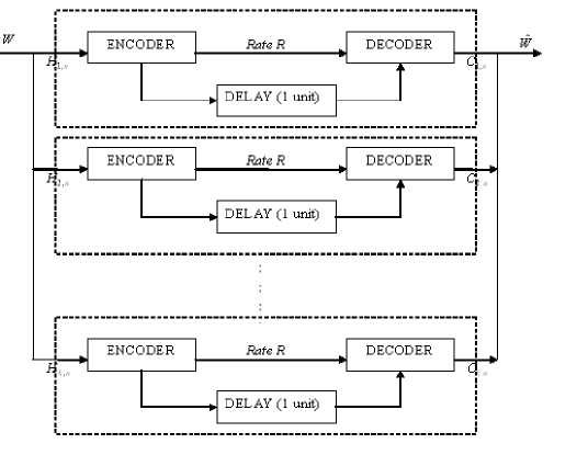
Figure 3: Directed Information setup under Source coding with feedforward

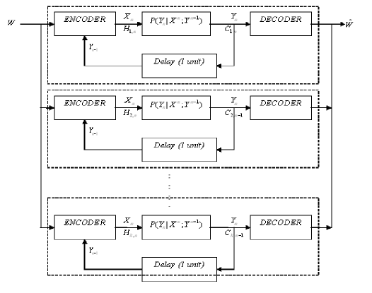
Figure 4: Directed Information setup under Channel Coding with feedback

A brief background about DTI is in order: Directed Information comes from a rich literature regarding capacity of channels with feedback or understanding rate-distortion theory in source coding with feedforward [19]. Source coding and channel coding are information-theoretic duals, and DTI is useful to characterize source or channel behavior when the information being transferred is correlated [20].

The relationship between MI and DTI is given by,
MI:  $I(X^{N};Y^{N})=\sum_{i=1}^{N}I(X^{n};Y_{i}|Y^{i-1})=I(X^{N}\rightarrow Y^{N})+I(0Y^{N-1}\rightarrow X^{N}).$
DTI:  $I(X^{N}\rightarrow Y^{N})=\sum_{i=1}^{N}I(X^{i};Y_{i}|Y^{i-1})$.

Just like the case where we maximize $I(X;Y)$ in channel coding, or minimize $I(X;Y)$ for source coding in cases without feedback, we maximize/minimize $I(X\rightarrow Y)$ in the corresponding cases with feedback/feedforward. This feature selection problem for the $i^{th}$ training instance becomes one of identifying which hexamer ($k\in(1,2,\ldots,4096)$) has the highest $I(X_{i,k}\rightarrow Y_{i})$ or the lowest $I(Y_{i}\rightarrow X_{i,k})$ if looked from the source or channel coding perspectives respectively.

In our case, we treat the hexamers ($X_{i}$) like messages and the class labels ($Y$) as the reconstruction after transmission and are interested in asking which messages transmit maximum information to the reconstructed versions. These are the features which maximally influence the class label. At each instant (in time or training iteration), the learning algorithm uses the previous associations between the hexamer features ($X_{k,1},X_{k,2},\ldots,X_{k,i-1}$) and corresponding class labels ($Y_{1},Y_{2},\ldots,Y_{i-1}$) to predict a class label ($\hat{Y}_{i}$) for the current hexamer feature instance ($X_{i}$). Following the concept of feedforward, the true class label $Y_{i}$ is then given to the algorithm (after the prediction $\hat{Y}_{i}$) is made. Based on the prediction ($\hat{Y}_{i}$) and the true class label $Y_{i}$, the algorithm will learn the hexamer-label associations up until the instance it has just observed (i.e. the $i^{th}$ instant), and so on. It does this for each hexamer ${}^{\prime}k^{\prime}$ in the feature vector, and finds the hexamer which has maximum association within this sequential learning paradigm (Figs 3 and 4). Each dotted box represents the DTI based feature learning for each hexamer. Thus, this is thought of $M=1000$ operations in parallel. The training iterations proceed as long as it takes to achieve a certain accuracy of classification. We would expect that DTI needs lesser number of features than MI to achieve the same classification rate.

The DTI (for a lag of 1) - which is a measure of the causal dependence between two random processes $X_{i}=[X_{1,i},X_{2,i},\ldots X_{n,i}]$, (with $X_{j,i}$ = quantile label for the frequency of hexamer $i\in(1,2,\ldots,1000)$ in the $j^{th}$ training sequence) and $Y=[Y_{1},Y_{2},\ldots,Y_{n}]$ being the corresponding class labels ($-1/+1$), is given by [6]:

$$I(X_{i}^{N}\rightarrow Y^{N})=\sum_{n=1}^{N}I(X_{i}^{n};Y_{n}|Y^{n-1}) 1$$ ()

Here, $N$ is $2N_{train}$, the total number of training data class labels. As already known, the mutual information $I(X;Y)=H(X)-H(X|Y)$, with $H(X)$ and $H(X|Y)$ being the Shannon entropy of $X$ and the conditional entropy of $X$ given $Y$, respectively. Using this definition of mutual information, the Directed Information simplifies to,

$$I(X^{N}\rightarrow Y^{N})=\sum_{n=1}^{N}[H(X^{n}|Y^{n-1})-H(X^{n}|Y^{n})]$$

$$=\sum_{n=1}^{N}\{[H(X^{n},Y^{n-1})-H(Y^{n-1})]-[H(X^{n},Y^{n})-H(Y^{n})]\} 2$$ ()

Using (2), the Directed information is expressed in terms of individual and joint entropies of $X$ and $Y$. For the purpose of entropy estimation, we can adopt several approaches. In this work we examine two different ways to estimate the directed information from the hexamer-sequence frequency matrix.

The first way is to bin each frequency vector into $L$ quantiles. Thus, within the $i^{th}$ sequence (promoter/LRE), we can find the distribution of the hexamers within the sequence and bin them into the appropriate quantile. The value/entry in each cell of Table I is $l\in(1,2,\ldots,L)$. The last element in the data vector is the class label ($-1/+1$). Hence, it is now straightforward to find the marginal and joint distributions for the $k^{th}$ hexamer ($X_{i,k}$) and the class label ($Y_{i}$).

An alternate method to find the joint information of the random variables $X^{N}$ and $Y^{N}$ uses the Darbellay-Vajda algorithm [7]. From $(2)$, we also have,

$$I(X^{N}\rightarrow Y^{N})=\sum_{n=1}^{N}[H(X^{n}|Y^{n-1})-H(X^{n}|Y^{n})]$$

$$=\sum_{n=1}^{N}[H(X^{n})-I(X^{n};Y^{n-1})]-[H(X^{n})-I(X^{n};Y^{n})]$$

$$(\text{using }I(X^{n};Y^{n})=H(X^{n})-H(X^{n}|Y^{n}))$$

$$=\sum_{n=1}^{N}[I(X^{n};Y^{n})-I(X^{n};Y^{n-1})]$$

$$=\sum_{n=1}^{N}[I(X^{n};Y^{n})-I(X^{n};0Y^{n-1})]$$

In the above expressions, the mutual information between two random variables in the sum ($I(X^{n};Y^{n})$ and $I(X^{n};0Y^{n-1})$) can be estimated using a non-parametric adaptive binning procedure ([35], [7]) by iterative partitioning of the observation space until conditional independence is achieved within and between partitions. This method lends itself to a tree based partitioning scheme and can be used for entropy estimation even for a moderate number of samples in the observation space of the underlying probability distribution. Several such algorithms for adaptive density estimation have been proposed ([32],[31],[33], [34]) and can find potential application in this procedure. Because of the higher performance guarantees in using this procedure as well as the relative ease of implementation, we use the Darbellay-Vajda approach for entropy (and information) estimation in our methodology.

Both these methods (equiquantization and Darbellay-Vajda) provide a way to estimate the true DTI between a given hexamer and the class label for the entire training set. Feature selection comprises of finding all those hexamers ($X_{i}$) for which $I(X_{i}\rightarrow Y)$ is the highest. From the definition of DTI, we know that $0\leq I(X_{i}\rightarrow Y)\leq I(X_{i};Y)<\infty$. To make a meaningful comparison of the strengths of association between different hexamers and the class label, we need to find a normalized score (Sec:$VII$) to rank the DTI values. Another point of consideration is that we need to ask how significant the DTI value is compared to a null distribution on the DTI value (i.e. what is the chance of finding the DTI value by chance from the series $X_{i}$ and $Y$). This is done using confidence intervals after permutation testing (Sec: $IX$).

A normalized DTI measure

In this section, we derive an expression for a ’normalized DTI coefficient’. This is useful for a meaningful comparison across different criteria during network inference. For now, we will compare the network influences as inferred from normalized DTI and CoD [14]. In this section, we use $X$,$Y$, $Z$ for $X^{N}$, $Y^{N}$ and $Z^{N}$ interchangeably, i.e $X\equiv X^{N}$, $Y\equiv Y^{N}$, and $Z\equiv Z^{N}$.

By the definition of DTI, we can see that $0\leq I(X^{N}\rightarrow Y^{N})<I(X^{N};Y^{N})<\infty$. The normalized measure $\rho_{DTI}$ should be able to map this large range ($[0,\infty]$) to $[0,1]$.

We recall that the multivariate canonical correlation is given by [26]: $\rho_{X^{N};Y^{N}}=\Sigma_{X^{N}}^{-1/2}\Sigma_{X^{N};Y^{N}}\Sigma_{Y^{N}}^{-1/2}$
and this is normalized having eigenvalues between 0 and 1. We also recall that, under a Gaussian distribution on $X^{N}$ and $Y^{N}$, the joint entropy $H(X^{N};Y^{N})=-\frac{1}{2}\ln(2\pi e)^{2N}|\Sigma_{X^{N}Y^{N}}|$, where $|A|$ is the determinant of matrix $A$, $\Sigma$ denotes the covariance matrix.

Thus, for $I(X^{N};Y^{N})=H(X^{N})+H(Y^{N})-H(X^{N};Y^{N})$, the expression for mutual information, under jointly Gaussian assumptions on $X^{N}$ and $Y^{N}$, becomes,
$I(X;Y)=-\frac{1}{2}\ln(\frac{|\Sigma_{X^{N}Y^{N}}|^{2}}{|\Sigma_{X^{N}}|.|\Sigma_{Y^{N}}|})=-\frac{1}{2}\ln(1-\rho_{X^{N};Y^{N}}^{2})$. Hence, a straightforward transformation is normalized MI, $\rho_{MI}=\sqrt{1-e^{-2I(X;Y)}}=\sqrt{1-e^{-2\sum_{i=1}^{N}I(X^{N};Y_{i}|Y^{i-1})}}$ . A connection with [27], can thus be immediately seen.

Both of these will be normalized between $(0,1)$ and will give a better absolute definition of dependency that does not depend on the unconditioned MI. We will use this definition of normalized information coefficients for the present set of simulation studies.

For constructing a normalized version of the DTI, we can extend this approach , from ([13], [27]). Consider three random vectors X, Y and Z, each of which are identically distributed as $\mathcal{N}(\mu_{X},\Sigma_{XX})$, $\mathcal{N}(\mu_{Y},\Sigma_{YY})$, and $\mathcal{N}(\mu_{Z},\Sigma_{ZZ})$ respectively. We also have,

$(\textbf{X},\textbf{Y},\textbf{Z})\sim\mathcal{N}\left[\left(\begin{array}[]{c}\mu_{X}\\ \mu_{Y}\\ \mu_{Z}\end{array}\right),\left(\begin{array}[]{ccc}\Sigma_{XX}&\Sigma_{XY}&\Sigma_{XZ}\\ \Sigma_{YX}&\Sigma_{YY}&\Sigma_{YZ}\\ \Sigma_{ZX}&\Sigma_{ZY}&\Sigma_{ZZ}\end{array}\right)\right]$

Their partial correlation $\delta_{YX|Z}$ is given by,
$\delta_{YX|Z}=\sqrt{\frac{a_{2}^{2}}{a_{1}a_{3}}}$ with,
$a_{1}=\Sigma_{YY}-\Sigma_{YZ}\Sigma_{ZZ}^{-1}\Sigma_{ZY}$, $a_{2}=\Sigma_{YX}-\Sigma_{YZ}\Sigma_{ZZ}^{-1}\Sigma_{ZX}$,
$a_{3}=\Sigma_{XX}-\Sigma_{XZ}\Sigma_{ZZ}^{-1}\Sigma_{ZX}$

Recalling results from conditional Gaussian distributions, these can be denoted by: $a_{1}=\Sigma_{Y|Z},a_{2}=\Sigma_{XY|Z}$ and $a_{3}=\Sigma_{X|Z}$.

Thus, $\delta_{YX|Z}=\Sigma_{Y|Z}^{-1/2}\Sigma_{XY|Z}\Sigma_{X|Z}^{-1/2}$. Extending the above result from the mutual information to the directed information case, we have, $\rho_{DTI}=\sqrt{1-e^{-2\sum_{i=1}^{N}I(X^{i};Y_{i}|Y^{i-1})}}$.

To once again clarify, we recall the primary difference between MI and DTI, (note the superscript on X)
MI:  $I(X^{N};Y^{N})=\sum_{i=1}^{N}I(X^{N};Y_{i}|Y^{i-1})=I(X^{N}\rightarrow Y^{N})+I(0Y^{N-1}\rightarrow X^{N})$.
DTI:  $I(X^{N}\rightarrow Y^{N})=\sum_{i=1}^{N}I(X^{i};Y_{i}|Y^{i-1})$.

Kernel Density Estimation (KDE)

The goal in density estimation is to find a probability density function $\hat{f}(z)$ that approximates the underlying density $f(z)$ of the random variable $Z$. Under certain regularity conditions, the kernel density estimator $\hat{f}_{h}(Z)$ at the point $x$ is given by $\hat{f}_{h}(Z)=\frac{1}{nh}\sum_{i=1}^{n}K(\frac{z_{i}-z}{h})$, with $n$ being the number of samples $z_{1},z_{2},\ldots,z_{n}$ from which the density is to be estimated, $h$ is the bandwidth of a kernel $K(\bullet)$ that is used during density estimation.

A Kernel density estimator at $z$ works by weighting the samples (in $(z_{1},z_{2},\ldots,z_{n})$) around $z$ by a kernel function (window) and counts the relative frequency of the weighted samples within the window width. As is clear from such a framework, the choice of kernel function $K(\bullet)$ and the bandwidth $h$ determines the fit of the density estimate.

Some figures of merit to evaluate various kernels are the asymptotic mean integrated squared error (AMISE), bias-variance characteristics and region of support [29]. It is preferred that a kernel have a finite range of support, low AMISE and a favorable bias-variance tradeoff. The bias is reduced if the kernel bandwidth (region of support) is small, but has higher variance because of a small sample size. For a larger bandwidth, this is reversed (ie large bias and smaller variance). Under these requirements, the Epanechnikov kernel has the most of these desirable characteristics - i.e. a compact region of support, the lowest AMISE compared to other kernels, and a favorable bias variance tradeoff [29].

The Epanechnikov kernel is given by:

$$K(u)=\frac{3}{4}(1-u^{2})I(\left|u\right|\leq 1).$$

with $I(\bullet)$ being the indicator function conveying a window of width spanning $[-1,1]$ centered at $0$. An optimal choice of the bandwidth is $h=1.06\times\hat{\sigma}_{z}\times n^{-1/5};$, following [[28]]. Here $\hat{\sigma}_{z}$ is the standard error from the bootstrap DTI samples $(z_{1},z_{2},\ldots,z_{n})$.

Hence the kernel density estimate for the bootstrapped DTI (with $n=1000$ samples), $Z\triangleq\hat{I}_{B}(X^{N}\rightarrow Y^{N})$ becomes,
$\hat{f}_{h}(Z)=\frac{1}{nh}\sum_{i=1}^{n}\frac{3}{4}[1-(\frac{z_{i}-z}{h})^{2}]I(\left|\frac{z_{i}-z}{h}\right|\leq 1)$ with $h\approx 2.67\hat{\sigma}_{z}$ and $n=1000$. We note that $\hat{I}_{B}(X^{N}\rightarrow Y^{N})$ is obtained by finding the DTI for each random permutation of $X$, $Y$ time series, and performing this permutation $B$ times.

VII Bootstrapped Confidence Intervals

Since we do not know the true distribution of the DTI estimate, we find an approximate confidence interval for the DTI estimate ($\hat{I}(X^{N}\rightarrow Y^{N})$), using bootstrap above [30].

We denote the cumulative distribution function (over the Bootstrap samples) of $\hat{I}(X^{N}\rightarrow Y^{N})$ by $F_{\hat{I_{B}}(X^{N}\rightarrow Y^{N})}(\hat{I_{B}}(X^{N}\rightarrow Y^{N}))$. Let the mean of the bootstrapped null distribution be $I_{B}^{*}(X^{N}\rightarrow Y^{N})$. We denote by $t_{1-\alpha}$, the $(1-\alpha)^{th}$ quantile of this distribution i.e. {$t_{1-\alpha}:P([\frac{\hat{I_{B}}(X^{N}\rightarrow Y^{N})-I_{B}^{*}(X^{N}\rightarrow Y^{N})}{\hat{\sigma}}]\leq t_{1-\alpha})=1-\alpha$}. Since we need the real $\hat{I}(X^{N}\rightarrow Y^{N})$ to be significant and as close to 1, we need $\hat{I}(X^{N}\rightarrow Y^{N})\geq[I_{B}^{*}(X^{N}\rightarrow Y^{N})+t_{1-\alpha}\times\hat{\sigma}]$, with $\hat{\sigma}$ being the standard error of the bootstrapped distribution,
$\hat{\sigma}=\sqrt{\frac{[\Sigma_{b=1}^{B}\hat{I_{b}}(X^{N}\rightarrow Y^{N})-I_{B}^{*}(X^{N}\rightarrow Y^{N})]^{2}}{B-1}}$; $B$ is the number of Bootstrap samples.

VIII Support Vector Machines

From the top $"d"$ features identified from the ranked list of features having high DTI with the class label, a hyperplane linear classifier in these $"d"$ dimensions is designed. A Support Vector Machine (SVM) is a hyperplane classifier which operates by finding a maximum margin linear hyperplane to separate two different classes of data in high dimensional ($D>"d"$) space. Our training data has $N_{train}$ pairs $(x_{1},y_{1}),(x_{2},y_{2}),\ldots,(x_{N_{train}},y_{N_{train}})$, with $x_{i}\in\mathscr{R}^{D}$ and $y_{i}\in\{-1,+1\}$.

An SVM is a maximum margin hyperplane classifier in a non-linearly extended high dimensional space. For extending the dimensions from $d$ to $D>d$, a radial basis kernel is used.

The objective is to minimize $||\beta||$ in the hyperplane $\{x:f(x)=x^{T}\beta+\beta_{0}\}$, subject to
$y_{i}(x^{T}_{i}\beta+\beta_{0})\geq 1-\xi_{i}\forall i$, $\xi_{i}\geq 0,\sum\xi_{i}\leq$ constant [29].

IX Summary of Overall Approach

Our proposed approach is as follows. Here, the term ’sequence’ can pertain to either tissue specific promoters or LRE sequences.

• Parse the sequence to obtain the relative counts/frequencies of occurrence of the hexamer in that sequence and build the hexamer-sequence frequency matrix. The ’seqinr’ package in R is used for this purpose. This is done for all the sequences in the specific (class $+1$) and non-specific (class $-1$) categories. The matrix thus has $N_{train}$ rows and $4^{6}=4096$ columns.

• Preprocess the obtained hexamer-sequence frequency matrix by finding the quantile labels for each hexamer within the $i^{th}$ sequence. We now have a hexamer-sequence matrix where the cell $(i,j)$ has the quantile label of the $j^{th}$ hexamer in the $i^{th}$ sequence. This is done for all the $N(=S_{ts}+S_{nts})$ training sequences consisting of examples from the $-1$ and $+1$ class labels.

• Build two submatrices corresponding to the two class labels. Thus one matrix will contain the hexamer-sequence quantile labels for the positive training examples and the other matrix is for the negative training examples.

• To pick the hexamers that are most different between the positive and negative training examples, we perform a paired t-test for each hexamer. Rank all the corresponding t-test p-values from lowest to highest and take the top $1000$ hexamers. These correspond to the $1000$ hexamers that are most different distributionally (in mean) between the positive and negative training samples. We note that the t-test requires the same number of samples in the positive ($S_{ts}$ samples) and negative ($S_{nts}$ samples) training set. Hence, we consider $N_{train}=min(S_{ts},S_{nts})$ examples for each of the positive and negative training cases. Another way to resolve this problem is to find the symmetrized KL divergence/ Jensen-Shannon divergence between the hexamer distributions of the positive and negative examples. This step is only necessary to reduce the computational complexity of the overall procedure - finding the DTI between each of the 4096 hexamers and the class label is very expensive.

• For the top $K=1000$ hexamers which are most significantly different between the positive and negative training examples, we proceed to find $I(X_{i,k}\rightarrow Y_{i})$ and $I(X_{i,k}\rightarrow Y_{i})$ for each of the $k\in(1,2,\ldots,K)$ hexamers. The entropy terms in the directed information and mutual information expressions can be found either from the equidistant binning approach or the Darbellay-Vajda approach. Since the goal is to maximize $I(X_{i,k}\rightarrow Y_{i})$ or minimize $I(Y_{i}\rightarrow X_{i,k})$, we can rank them in descending and ascending order, respectively. Using the procedure of Section.VII, the raw DTI values can be converted into their normalized versions.

• We also find the significance of the DTI estimate obtained in the step above. Thus if we set a threshold of $0.05$ significance, we can take every hexamer whose DTI is $0.05$ significant with respect to its bootstrapped null distribution (using kernel density estimation), and rank the hexamers by decreasing DTI value. The top $"d"$ hexamers in this ranked list can be used for classifier (SVM) training.

• We now train the Support Vector Machine classifier (SVM) on the top $"d"$ features from the ranked DTI list(s). For comparison with the MI based technique, we use the hexamers which have the top $"d"$ (normalized) MI values. We can now plot the accuracy of the trained classifier as a function of the number of features ($d$). As we gradually consider higher $"d"$, we move down the ranked list.

X Results

X-A Tissue specific promoters

We use DTI to find discriminating hexamers that underlie brain specific and heart specific expression.

Results for the MI and DTI methods are given below (Figs.5 and 6). The plots indicate the cross-validated misclassification accuracy (ideally $0$) for the data as the number of features using the metric (DTI or MI) is gradually increased. We can see that for any given classification accuracy, the number of features using DTI is less than the corresponding number of features using MI. This translates into a lower misclassification rate for DTI-based feature selection. We observe that as the number of features $"d"$ is increased the performance of MI is the same as DTI.

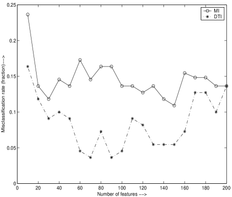
Figure 5: Misclassification accuracy for the MI vs. DTI case (brain promoter set)

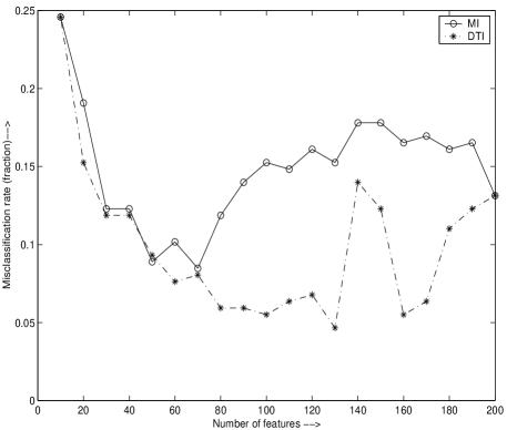
Figure 6: Misclassification accuracy for the MI vs. DTI case (heart promoter set)

Some of the key motifs in the heart and brain case are given in Table II. Wherever possible, we indicate if the motif corresponds to a known transcription factor binding motif. We note that just because a motif corresponds to a transcription factor binding site (TFBS), it does not imply that the TF is functional in brain or heart. It might however, be useful to do focused experiments to check their functional role.

Brain	Heart	Brain
-promoters	promoters	enhancers
Ahr-ARNT	Pax2	HNF-4
Tcf11-MafG	Tcf11-MafG	Nkx
c-ETS	XBP1	AML1
FREAC-4	Sox-17	c-ETS
T3R-alpha1	FREAC-4	Elk1

TABLE II: Comparison of high ranking motifs (by DTI) across different data sets.

X-B Enhancer DB

We examine all the brain -specific regulatory elements profiled in the EnhancerDB database (http://http://enhancer.lbl.gov/) for discriminating motifs. Again, the plot of misclassification accuracy vs. number of features in the MI and DTI scenarios are indicated in Figs. 5-7.

Figure 7: Misclassification accuracy for the MI vs. DTI case (brain enhancer set)

Some of the top ranking motifs from this dataset are also shown in Table II.

XI Other Applications

We now proceed to show other related applications wherein the DTI based learning framework is useful. Compared to other approaches we can investigate the role of ’any’ motif (possibly a transcription factor binding motif) both in sequence or via expression data. We illustrate this via an example.

XI-A

Suppose we are interested in the transcription factors that regulate Gata3 gene expression. This gene has expression in the developing kidney, central nervous systems and hematopoietic cell differentiation. In concordance with the established framework of transcription presented in Section I, recruitment of TFs happens at both the proximal promoter as well as long-range regulatory elements. A common approach to find functional TFBSes from the promoter sequence is to look for phylogenetically conserved TF binding sites in the promoter sequence among species in which Gata3 is involved in the same biological process (here kidney development).

Figure 8: Cumulative Distribution Function for bootstrapped $I(\textit{Pax2}\rightarrow\textit{Gata3})$. True $\hat{I}(\textit{Pax2}\rightarrow\textit{Gata3})=0.9911$.

As shown above, this DTI is seen to be significant and strong. DTI also enables the integration of microarray time series data expression (from the developing kidney) of the Pax2 gene to ask if there is any influence from Pax2 to Gata3. This is not discussed here but some preliminary work is available in [3].

Figure 9: Cumulative Distribution Function for bootstrapped $I(\textit{Pax2 motif:GTTCC}\rightarrow Y)$; $Y$ is the class label (UB/non-UB). True $\hat{I}(\textit{Pax2}\rightarrow\textit{Gata3})=0.9792$.

XI-B

The other question again picks up on something quite traditionally done in bioinformatics research - finding key TF regulators underlying tissue-specific expression. Again, using the Gata3 gene as an example, it has been observed that it is expressed in the developing ureteric bud (UB) during kidney development. To find UB specific regulators, we look for conserved TF modules in the promoters of UB-specific genes. These experimentally annotated UB-specific genes are obtained from the Mouse Genome Informatics database at http://www.informatics.jax.org/. Several programs are used for this kind of analysis, like Genomatix [25] or Toucan [24]. Using Toucan, we align the promoters of the various UB specific genes, and obtained several related modules. The top-ranking module in Toucan contains AHR-ARNT, Hox13, Pax2, Tal1alpha-E47, Oct1. We can now check if the corresponding motifs can discriminate UB-specific and non-specific genes, from DTI.

We can now check if the Pax2 binding motif (GTTCC [18]) induces kidney specific expression by looking for the strength of DTI between the GTTCC motif and the class label ($+1$) indicating UB expression. This once again adds to computational evidence for the true role of Pax2 in directing ureteric bud specific expression [18].

XII Discussion

From the results above, we observe that the average misclassification error is higher in the heart/brain promoter datasets than for the enhancer data. We speculate this is due to a number of reasons:

• There is more sequence variability at the promoter since it has to act in concert with LREs of different tissue types.

• Since the enhancer/LRE acts with the promoter to confer expression in only one tissue type, these sequences are more specific and hence their mining identifies motifs that are probably more indicative of tissue-specific expression.

We however, reiterate that the enhancer dataset that we study always make use of the hsp68-lacz as the promoter driven by the ultraconserved elements. Hence we do not have promoter specificity. Though this is a disadvantage and might not reveal all key motifs, it is the best that can be done in the absence of any other comprehensive repository.

XIII Conclusions

In this work, we have presented a framework for the identification of hexamer motifs to discriminate between two kinds of sequences (tissue-specific promoters vs non-specific or tissue-specific regulatory elements vs non-specific). For this feature selection problem we proposed the utility of a new metric - the ’directed information’ (DTI). In conjunction with a support vector machine classifier, this method was shown to outperform the state of the art methods employing ordinary mutual information. We also find that only a subset of the discriminating motifs correlate with known transcription factor motifs and hence might be potentially related to underlying epigenetic phenomena governing tissue-specific expression. The superior performance of the directed-information based variable selection suggests its utility to more general sequential learning problems.

We also examine the applicability of DTI for questions focusing on any motif of interest, obtained as output from other sources (literature, expression data, module searches). Thus one can prospectively resolve the role of a TF in a biological process.

XIV Acknowledgements

The authors gratefully acknowledge the support of the NIH under award 5R01-GM028896-21 (J.D.E). We would also like to thank Prof. Sandeep Pradhan and Mr. Ramji Venkataramanan for useful discussions on Directed information.

References

- [1] Stuart RO, Bush KT, Nigam SK, ”Changes in gene expression patterns in the ureteric bud and metanephric mesenchyme in models of kidney development”, Kidney International,64(6),1997-2008,December 2003.
- [2] Chan BY, Kibler D.,Using hexamers to predict cis-regulatory motifs in Drosophila.,BMC Bioinformatics. 2005 Oct 27;6:262.
- [3] Rao,Hero AO,States DJ,Engel JD,”Inference of biologically relevant Gene Influence Networks using the Directed Information Criterion”,Proc. of the IEEE Conference on Acoustics, Speech and Signal Processing, 2006.
- [4] Casella G. and Berger RL. ”Statistical Inference”, Duxbury Press, 1990.
- [5] Hutchinson GB.,”The prediction of vertebrate promoter regions using differential hexamer frequency analysis”.,Comput Appl Biosci. 1996 Oct;12(5):391-8.
- [6] NCBI Pubmed URL: http://www.ncbi.nlm.nih.gov/entrez/query.fcgi
- [7] G. A. Darbellay and I. Vajda, ”Estimation of the information by an adaptive partitioning of the observation space,” IEEE Trans. on Information Theory, vol. 45, pp. 1315–1321, May 1999.
- [8] Hastie T, Tibshirani R,The Elements of Statistical Learning , Springer 2002.
- [9] F. Fleuret. ”Fast binary feature selection with conditional mutual information”, Journal of Machine Learning Research,, 1531 1555, 2004.
- [10] I. Guyon, A. Elisseeff, ”An Introduction to Variable and Feature Selection”, Journal of Machine Learning Research 3 1157-1182,
- [11] Kadota K, Ye J, Nakai Y, Terada T, Shimizu K.,”ROKU: a novel method for identification of tissue-specific genes”,.2003. BMC Bioinformatics. 2006 Jun 12;7:294.
- [12] Schug , J., Schuller, W-P., Kappen, C., Salbaum, J.M., Bucan, M., Stoeckert, C.J. Jr.,”Promoter Features Related to Tissue Specificity as Measured by Shannon Entropy”., Genome Biology 6(4): R33, March 2005.
- [13] Geweke J.,”The Measurement of Linear Dependence and Feedback Between Multiple Time Series,” Journal of the American Statistical Association, 1982, 77, 304-324. (With comments by E. Parzen, D. A. Pierce, W. Wei, and A. Zellner, and rejoinder)
- [14] R. Hashimoto, E.R.Dougherty, M. Brun, Z. Zhou, M.L. Bittner, J.M. Trent, ”Efficient selection of feature-sets possessing hig coefficients of determination based on incremental determinations”,Signal Processing. 83 (4) (2003) 695-712.
- [15] Ghosh D, Chinnaiyan AM., ”Classification and selection of biomarkers in genomic data using LASSO”.,J Biomed Biotechnol., 2005(2):147-54.
- [16] Trindade LM, van Berloo R, Fiers M, Visser RG.,”PRECISE: software for prediction of cis-acting regulatory elements”.,J Hered. 2005 Sep-Oct;96(5):618-22.
- [17] Proc. NIPS 2006 Workshop on Causality and Feature Selection, available at: http://research.ihost.com/cws2006/
- [18] Dressler, G.R. and Douglas, E.C. (1992)., ”Pax-2 is a DNA-binding protein expressed in embryonic kidney and Wilms tumor”., Proc. Natl. Acad. Sci. USA 89: 1179-1183.
- [19] J. Massey, ”Causality, feedback and directed information,” Proc. 1990 Symp. Information Theory and Its Applications (ISITA-90), Waikiki, HI, Nov. 1990, pp. 303 305.
- [20] Pradhan, S. S., ”On the Role of Feedforward in Gaussian Sources: Point-to-Point Source Coding and Multiple Description Source Coding,” Information Theory, IEEE Transactions on Information Theory , vol.53, no.1pp.331-349, Jan. 2007.
- [21] Burge C, Karlin S: ”Prediction of complete gene structures in human genomic DNA”. J Mol Biol 1997, 268:78-94.
- [22] King DC, Taylor J, Elnitski L, Chiaromonte F, Miller W, Hardison RC., ”Evaluation of regulatory potential and conservation scores for detecting cis-regulatory modules in aligned mammalian genome sequences”.,Genome Res. 2005 Aug;15(8):1051-60. Epub 2005 Jul 15.
- [23] Pennacchio, L. A., Ahituv, N., Moses, A., Prabhakar, S., Nobrega, M., Shoukry, M., Minovitsky, A., Dubchak, I., Holt, A., Lewis, K., Plazer-Frick, I., Akiyama, J., DeVal, S., Afzal, V., Black, B., Couronne, O., Eisen, M., Visel, A., and Rubin, E.M. 2006., ”In vivo enhancer analysis of human conserved non-coding sequences”, Nature, 444(7118):499-502.
- [24] Aerts S, Van Loo P, Thijs G, Mayer H, de Martin R, Moreau Y, De Moor B.,TOUCAN 2: the all-inclusive open source workbench for regulatory sequence analysis.,Nucleic Acids Res. 2005 Jul 1;33(Web Server issue):W393-6.
- [25] Werner T., ”Regulatory networks: Linking microarray data to systems biology”.,Mech Ageing Dev. 2007 Jan;128(1):168-72.
- [26] Gubner J. A., Probability and Random Processes for Electrical and Computer Engineers, Cambridge, 2006.
- [27] H. Joe., ”Relative entropy measures of multivariate dependence”. J. Am. Statist. Assoc., 84:157 164, 1989.
- [28] J. Ramsay, B. W. Silverman, Functional Data Analysis (Springer Series in Statistics), Springer 1997.
- [29] Hastie T, Tibshirani R, The Elements of Statistical Learning , Springer 2002.
- [30] Effron B, Tibshirani R.J, An Introduction to the Bootstrap (Monographs on Statistics and Applied Probability), Chapman & Hall/CRC, 1994.
- [31] Nemenman, F Shafee, and W Bialek. ”Entropy and inference, revisited.”, In TG Dietterich, S Becker, and Z Ghahramani, editors, Advances in Neural Information Processing Systems 14, Cambridge, MA, 2002. MIT Press.
- [32] Willett R, Nowak R, ”Complexity-Regularized Multiresolution Density Estimation”, ISIT 2004.
- [33] Paninski, L. (2003)., ”Estimation of entropy and mutual information”. Neural Computation 15: 1191-1254.
- [34] Erik Learned-Miller and John W. Fisher, III. ”ICA using spacings estimates of entropy”. Journal of Machine Learning Research (JMLR), Volume 4, pp. 1271-1295, 2003.
- [35] Hudson, J.E., ”Signal Processing Using Mutual Information”, Signal Processing Magazine,Volume: 23,no: 6 pp:50-54, Nov. 2006.
- [36] Visel A, Minovitsky S, Dubchak I, Pennacchio LA., ”VISTA Enhancer Browser–a database of tissue-specific human enhancers”., Nucleic Acids Res. 2007 Jan;35(Database issue):D88-92.
- [37] Pennacchio LA, Loots GG, Nobrega MA, Ovcharenko I., ”Predicting tissue-specific enhancers in the human genome”., Genome Res. 2007 Jan 8;
- [38] Prabhakar S, Poulin F, Shoukry M, Afzal V, Rubin EM, Couronne O, Pennacchio LA., ”Close sequence comparisons are sufficient to identify human cis-regulatory elements”., Genome Res. 2006 Jul;16(7):855-63.
- [39] Kleinjan DA, van Heyningen V., ”Long-range control of gene expression: emerging mechanisms and disruption in disease”., Am J Hum Genet. 2005 Jan;76(1):8-32.
- [40] Khandekar M, Suzuki N, Lewton J, Yamamoto M, Engel JD., ”Multiple, distant Gata2 enhancers specify temporally and tissue-specific patterning in the developing urogenital system”.,Mol Cell Biol. 2004 Dec;24(23):10263-76.
- [41] Lakshmanan, G., K. H. Lieuw, K. C. Lim, Y. Gu, F. Grosveld, J. D. Engel, and A. Karis. 1999. ”Localization of distant urogenital system-, central nervous system-, and endocardium-specific transcriptional regulatory elements in the GATA-3 locus”. Mol. Cell. Biol. 19:1558-1568.
- [42] Lieb JD, Beck S, Bulyk ML, Farnham P, Hattori N, Henikoff S, Liu XS, Okumura K, Shiota K, Ushijima T, Greally JM., ”Applying whole-genome studies of epigenetic regulation to study human disease”.,Cytogenet Genome Res. 2006;114(1):1-15.
- [43] Kreiman G., ”Identification of sparsely distributed clusters of cis-regulatory elements in sets of co-expressed genes”.,Nucleic Acids Res. 2004 May 20;32(9):2889-900.
- [44] MacIsaac KD, Fraenkel E., ”Practical strategies for discovering regulatory DNA sequence motifs”.,PLoS Comput Biol. 2006 Apr;2(4):e36.
- [45] Peng H.,Long F.,Ding C.,”Feature Selection Based on Mutual Information: Criteria of Max-Dependency, Max-Relevance, and Min-Redundancy”, IEEE Transactions on Pattern Analysis and Machine Intelligence, vol. 27, No. 8, pp: 1226-1238, August 2005.