Bistability preserving model reduction in apoptosis

Abstract

Biological systems are typically very complex and need to be reduced before they are amenable to a thorough analysis. Also, they often possess functionally important dynamic features like bistability. In model reduction, it is sometimes more desirable to preserve the dynamic features only than to recover a good quantitative approximation. We present an approach to reduce the order of a bistable dynamical system significantly while preserving bistability and the switching threshold. These properties are important for the operation of the system in the context of a larger network. As an application example, a bistable model for caspase activation in apoptosis is considered.

, , , and

1 Introduction

The importance of switch–like decisions in biological processes has been revealed in a wide range of systems. Examples range from cell fate decisions via the MAP kinase cascade (Ferrell and Xiong, 2001) or apoptosis (Eißing et al., 2004) to changes of metabolic parameters, as e.g. induced by the lac operon (Yildirim et al., 2004). Switch–like decisions are also a major feature of more complex dynamics, as found for oscillations in the cell cycle (Pomerening et al., 2003). Concerning the mathematical modeling, switch–like decisions are usually represented by bistable dynamical systems. These systems have two stable steady states, and depending on initial conditions or external stimuli, converge to one of these steady states. Several theoretical approaches have been developed to study the existence of two stable steady states in dynamical systems (Angeli and Sontag, 2004; Eißing et al., 2007).

Another important issue in the modeling of biological systems is model reduction (Conzelmann et al., 2004). Due to the complexity of biological systems, typically only simplified models are amenable to a thorough computational analysis. Methods for model reduction which are theoretically founded provide important means to approximate a detailed description of a system by a simpler model.

Complex biological systems can often be viewed as a set of interconnected modules, each playing a specific role. In this case, two goals for model reduction of single modules can be distinguished. The first goal is to get a good quantitative approximation of the original model, such that a solution of the reduced model will differ as little as possible from a solution of the full model in the relevant variables (e.g. model outputs). For biochemical systems, this is often achieved via a time scale separation (e.g. Roussel and Fraser, 2001). The second goal focusses on preserving the qualitative dynamics of a module and its role in the network (Dano et al., 2006). In large biological networks, which typically are robust against fluctuations, the exact trajectories of the module might not be relevant, provided its qualitative behavior is preserved such that it can maintain its role in the network. When pursuing the latter goal, one can anticipate a much larger reduction than for the first one. For modules having the role of switches, the goal is thus to reduce the model while preserving bistability and the quantitative properties that are important for the module’s operation, like the switching threshold.

Based on a method introduced by Schmidt and Jacobsen (2004), which allows to compute a measure of the contribution of each state variable in the model to bistability, we present an approach for model reduction preserving bistability in switch–like systems. The method is applied to a bistable system involved in programmed cell death. We show that the reduction preserves not only bistability, but also quantitative properties like the linear approximation to the manifold separating the two regions of attraction of the stable steady states, which is related to the switching threshold of the system.

2 The caspase activation model

We study a model for caspase activation, a major part of apoptosis, developed by Eißing et al. (2004). Apoptosis, also called programmed cell death, is a signaling program that leads the cell to commit suicide under appropriate internal and/or external stimuli. It provides a living organism with means to remove infected, malfunctioning or simply unneeded cells to ensure its survival. Malfunction of apoptotic signaling has been detected in several diseases, including developmental defects, neurodegeneration and cancer (Danial and Korsmeyer, 2004). Therefore it is also of medical interest to understand the signaling network which regulates apoptosis.

Cell death is a switch–like decision: based on the input signal, the cell has to decide whether to undergo apoptosis or to stay alive. There is no gradual response. The role of the switching element in apoptosis is taken by the caspase cascade. One distinguishes initiator caspases which receive the stimuli and effector caspases actually carrying out apoptosis. Bistability in the model arises from a positive feedback loop between the effector caspases and the initiator caspases, in connection with the specific inhibitors for each type of caspases.

The model as developed by Eißing et al. (2004) already contains several simplifications, in particular several types of initiator and effector caspases are combined in one species each, and the same applies to several types of inhibitors of the effector caspases. Furthermore, the external stimulus is not explicitly included as an input, but instead the initial amount of activated initiator caspases resulting from the stimulation is considered as input to the model.

The species present in the model are the initiator caspase 8 and the effector caspase 3, both in active (C8a, C3a) and inactive (C8, C3) forms, and the inhibitors IAP and CARP as well as their complexes with active caspase 3 and 8, respectively. Figure 1 displays the species involved in the model and the reactions among them. The variables in the mathematical model denote the molecule numbers per cell of the various species (Table 1).

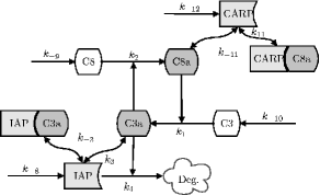
Figure 1: Representation of the caspase activation model. Constitutive degradation reactions are not displayed.

$\begin{aligned} x_{1}&=[\texttt{C8}]\\ x_{2}&=[\texttt{C8a}]\\ x_{3}&=[\texttt{C3}]\\ x_{4}&=[\texttt{C3a}]\end{aligned}$

$\begin{aligned} \quad x_{5}&=[\texttt{IAP}]\\ \quad x_{6}&=[\texttt{C3a\_IAP}]\\ \quad x_{7}&=[\texttt{CARP}]\\ \quad x_{8}&=[\texttt{C8a\_CARP}]\end{aligned}$

Table 1: Model state variables.

The equations for the caspase activation model are given in Table 2 with parameter values as shown in Table 3 (Eißing et al., 2004). These parameter values have been collected from literature. For simplicity, we consider state variables (given in molecules per cell) as dimensionless.

$$\dot{x}_{1} =-k_{2}x_{1}x_{4}-k_{9}x_{1}+k_{-9}$$ (1)

$$\dot{x}_{2} =k_{2}x_{4}x_{1}-k_{5}x_{2}-k_{11}x_{2}x_{7}+k_{-11}x_{8}$$

$$\dot{x}_{3} =-k_{1}x_{2}x_{3}-k_{10}x_{3}+k_{-10}$$

$$\dot{x}_{4} =k_{1}x_{2}x_{3}-k_{3}x_{4}x_{5}+k_{-3}x_{6}-k_{6}x_{4}$$

$$\dot{x}_{5} =-k_{3}x_{4}x_{5}+k_{-3}x_{6}-k_{4}x_{4}x_{5}-k_{8}x_{5}+k_{-8}$$

$$\dot{x}_{6} =k_{3}x_{4}x_{5}-k_{-3}x_{6}-k_{7}x_{6}$$

$$\dot{x}_{7} =-k_{11}x_{2}x_{7}+k_{-11}x_{8}-k_{12}x_{7}+k_{-12}$$

$$\dot{x}_{8} =k_{11}x_{2}x_{7}-k_{-11}x_{8}-k_{13}x_{8}$$

Table 2: Model equations

$k_{1}$	$5.8\cdot 10^{-5}$	$k_{11}$	$5\cdot 10^{-4}$
$k_{2}$	$1\cdot 10^{-5}$	$k_{12}$	$1\cdot 10^{-3}$
$k_{3}$	$5\cdot 10^{-4}$	$k_{13}$	$1.16\cdot 10^{-2}$
$k_{4}$	$3\cdot 10^{-4}$	$k_{-3}$	$0.21$
$k_{5}$	$5.8\cdot 10^{-3}$	$k_{-8}$	$464$
$k_{6}$	$5.8\cdot 10^{-3}$	$k_{-9}$	$507$
$k_{7}$	$1.73\cdot 10^{-2}$	$k_{-10}$	$81.9$
$k_{8}$	$1.16\cdot 10^{-2}$	$k_{-11}$	$0.21$
$k_{9}$	$3.9\cdot 10^{-3}$	$k_{-12}$	$540$
$k_{10}$	$3.9\cdot 10^{-3}$

Table 3: Parameter values $[\mathrm{min}^{-1}]$

The model yields two stable steady states, which can be identified with the living state, where the concentrations of all active caspases—both free and bound—are equal to zero, and with the apoptotic state where an almost complete activation of the caspases determines the cell to undergo apoptosis. The model captures the switch–like behavior occurring during apoptosis very well and is thus suitable to our needs.

Furthermore, we have a threshold manifold separating the regions of attraction, as well as an unstable steady state on the threshold manifold which we refer to as the decision state, as it is relevant in the decision about the fate of the cell.

3 Determination of relevance

When determining the relevance of each state variable in the system to bistability, the unstable steady state, or decision state, plays a crucial role. The boundaries of the bistability region in parameter space are marked by bifurcations of the unstable steady state and thus can in principle be detected by a classical bifurcation analysis. Although bifurcation analysis reveals the influence of parameters on the bistability, it does not give the relevance of each variable and how these are interconnected to generate bistability.

Based on a linear approximation of the model around the decision state, Schmidt and Jacobsen (2004) perturb the influence of one state variable on the other variables of the system. In the unperturbed case, the linear approximation is unstable, since the decision state is unstable. One now searches for a perturbation that renders the decision state stable, which would roughly correspond to reaching a bifurcation point in the original nonlinear system. The magnitude of a perturbation found in this way is then a measure of the relevance to bistability of the perturbed variable with its connections to other variables.

To make this approach precise, consider a system given by the differential equation

$$\frac{d}{dt}x=f(x),$$ (2)

with $x\in\mathbb{R}^{n}$. We assume that the system is bistable and has an unstable steady state $x_{d}$, the decision state for the bistable behavior. Setting $\Delta x=x-x_{d}$, the linearization around the decision state is given by

$$\frac{d}{dt}(\Delta x)=A\Delta x,$$ (3)

with $A=\frac{\partial f}{\partial x}(x_{d})$. Note that, by our assumption, the system (3) is unstable.

The linearized system is then considered as a closed feedback loop, in the sense that all interconnections between the state variables are put into a virtual feedback path. Breaking this feedback path yields the control system

$$L:\quad\frac{d}{dt}(\Delta x)=\tilde{A}\Delta x+(A-\tilde{A})u,$$

with $u\in\mathbb{R}^{n}$ and

$$\tilde{A}=\begin{pmatrix}a_{11}&&0\\ &\ddots&\\ 0&&a_{nn}\end{pmatrix},$$

i.e. $\tilde{A}$ contains only the elements on the diagonal of $A$. By setting $u=\Delta x$, the feedback path is closed again and one obtains the original linear system (3).

Following Schmidt and Jacobsen, we assume that the matrix $\tilde{A}$ is stable, i.e. $a_{ii}<0$ for $i=1,\ldots,n$. This implies that the instability of the closed loop system (3) is due to interconnections among variables.

Figure 2: Closed feedback loop with one feedback path perturbed

The computation is then done as follows: for each state variable $x_{i}$, a perturbation $\epsilon_{i}$ is introduced into the feedback path of this variable (Fig. 2). This yields the system

$$L_{i}(\epsilon_{i}):\quad\frac{d}{dt}(\Delta x)=A\Delta x+(A_{i}-\tilde{A}_{i})\epsilon_{i}\Delta x_{i},$$

where $A_{i}$ and $\tilde{A}_{i}$ are the $i$-th column of $A$ and $\tilde{A}$, respectively.

We are now searching for the minimal perturbation that will stabilize the system $L_{i}$ and define the value $\bar{\epsilon}_{i}$ as

$$\bar{\epsilon}_{i}=\min\{\epsilon_{i}>0\mid L_{i}(\epsilon_{i})\text{ or }L_{i}(-\epsilon_{i})\text{ is stable}\}.$$ (4)

If the minimum does not exist, set $\bar{\epsilon}_{i}=\infty$. The higher the value of $\bar{\epsilon}_{i}$, the more difficult it becomes to perturb the connections among the considered state variable $x_{i}$ and the remaining variables such that instability is lost, and the less relevant the variable $x_{i}$ is to bistability. Formally, we use the following definition of relevance.

Definition 1

The relevance $R_{i}$ of the state variable $x_{i}$ to the bistability of the system (2) is

$$R_{i}=\frac{1}{\bar{\epsilon}_{i}},$$

where $\bar{\epsilon}_{i}$ is given by equation (4).

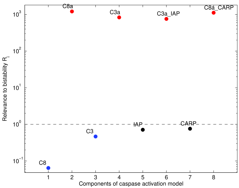
Figure 3: Relevance of components to bistability in the caspase activation model

This computation has been implemented numerically in the Systems Biology toolbox for Matlab (Schmidt and Jirstrand, 2006) and has been applied to the model of caspase activation described in Section 2. The result is shown in Fig. 3, and one distinguishes easily the relevant components C8a, C3a, C3a_IAP and C8a_CARP from the others, which are much less relevant to bistability.

It might be possible to develop a formal approach to compute $\bar{\epsilon}$ in equation (4) based on the Kharitonov theorem and its extensions (Bhattacharyya et al., 1995). However, the cost of computing a stabilizing perturbation would be similar to the one of a direct numerical search, since we consider only one perturbation at a time. Thus this idea is not pursued here.

4 Bistability preserving model reduction

Based on the measure of relevance presented in the previous section, we now develop a method of model reduction which preserves bistability in the reduced model. This reduction method is then applied to the caspase activation model (1).

4.1 Method of model reduction

The basic idea of the model reduction already used by Schmidt and Jacobsen (2004) is to retain only the state variables which have been identified as relevant to the bistability, and to neglect the dynamics of the other variables. In contrast to Schmidt and Jacobsen, who replace the neglected state variables in the remaining equations with their steady state values, we use their steady state map which is computed from the full model. Our approach will be justified in Section 4.2.

The relevant state variables can be identified by choosing appropriate thresholds $r>0$ for the relevance and $\alpha>1$ which determines the gap size.

Definition 2

The state variable $x_{i}$, $i=1,\ldots,n$, is said to be relevant (resp., irrelevant) to bistability, if there exist $r>0$ and $\alpha>1$ such that $R_{i}>\alpha r$ (resp., $R_{i}<\frac{1}{\alpha}r$).

Using this definition, the state $x$ of the system (2) is subdivided as

$$x\rightarrow(x_{R},x_{I})^{\mathrm{T}},$$

where $x_{R}$ contains the relevant variables and $x_{I}$ the irrelevant ones. Note that $\alpha$ should not be chosen to small to get a clear distinction between relevant and irrelevant state variables.

We then proceed as follows:

1. For each variable which is not relevant to bistability, compute its steady state map from the full model, i.e. solve the equation

   $$0=f(x_{R},x_{I})$$ (5)

   for $x_{I}$ to find the steady state map

   $$x_{I}=g(x_{R}).$$ (6)

   Computationally, this is similar to the division of a system in fast and slow subsystems using a quasi-steady-state approximation (Schauer and Heinrich, 1983), though we do not have fast and slow subsystems here, but rather subsystems that are relevant or irrelevant to bistability. The map $f$ has to be invertible with respect to $x_{I}$, which is the case in our example. Local invertibility can be checked via the implicit function theorem, but easily checkable conditions for global invertibility are not available in general.

2. Drop the differential equations for $x_{I}$ from the system and replace the components of $x_{I}$ in $f_{R}$ by their steady state map $g(x_{R})$.

   The reduced model is thus given by

   $$\dot{x}_{R}=f_{R}(x_{R},g(x_{R})).$$

To apply the described method to the model of caspase activation (1), we choose $r=10$ and $\alpha=10$. This yields the separation

$$x_{R}=(x_{2},x_{4},x_{6},x_{8})^{\mathrm{T}}\ \text{and}\ x_{I}=(x_{1},x_{3},x_{5},x_{7})^{\mathrm{T}}.$$

For the first step in the reduction, one gets the steady state map for $x_{I}$ as

$$x_{1} =\frac{k_{-9}}{k_{9}+k_{2}x_{4}} \quad x_{3} =\frac{k_{-10}}{k_{10}+k_{1}x_{2}}$$ (7)

$$x_{5} =\frac{k_{-8}+k_{-3}x_{6}}{(k_{3}+k_{4})x_{4}+k_{8}} \quad x_{7} =\frac{k_{-12}+k_{-11}x_{8}}{k_{12}+k_{11}x_{2}}$$

and the dynamics for the reduced model are thus given by

$$\dot{x}_{2} =\frac{k_{-9}k_{2}x_{4}}{k_{9}+k_{2}x_{4}}-k_{5}x_{2}-\frac{(k_{-12}+k_{-11}x_{8})k_{11}x_{2}}{k_{12}+k_{11}x_{2}}+k_{-11}x_{8}$$ (8)

$$\dot{x}_{4} =\frac{k_{-10}k_{1}x_{2}}{k_{10}+k_{1}x_{2}}-\frac{(k_{-8}+k_{-3}x_{6})k_{3}x_{4}}{(k_{3}+k_{4})x_{4}+k_{8}}+k_{-3}x_{6}-k_{6}x_{4}$$

$$\dot{x}_{6} =\frac{(k_{-8}+k_{-3}x_{6})k_{3}x_{4}}{(k_{3}+k_{4})x_{4}+k_{8}}-k_{-3}x_{6}-k_{7}x_{6}$$

$$\dot{x}_{8} =\frac{(k_{-12}+k_{-11}x_{8})k_{11}x_{2}}{k_{12}+k_{11}x_{2}}-k_{-11}x_{8}-k_{13}x_{8}.$$

Note that, in addition to the reduction in system dimension, also the dimension of the parameter space can be reduced: setting $\tilde{k}_{9}=k_{9}/k_{2}$ and $\tilde{k}_{10}=k_{10}/k_{1}$, the number of independent parameters in the model is reduced by two.

4.2 Results of reduction and interpretation

Analyzing the dynamics of the reduced model, one gets the following important results:

• All steady states of the full model are reproduced as a projection in the reduced model.

• The steady states of the reduced model have the same local stability behavior, in particular the same number of eigenvalues with positive real parts as their corresponding steady states in the full model after linearization.

• The linear approximation to the stable manifold at the decision state is the same up to projection for both the full and the reduced model.

The first property is obtained automatically by keeping the steady state map (7) of the neglected variables, under the assumption that no two steady states are projected to the same state by the reduction. Then one directly achieves the preservation of all steady states, which is a necessary condition for preservation of bistability. At this point, the change we made to the original approach of Schmidt and Jacobsen (2004) is important. Replacing the neglected variables with their constant steady state values does in general not preserve steady states other than the unstable decision state, in particular it does not preserve the two stable steady states in the caspase activation model. But to preserve bistability, it is not only necessary to preserve instability of the decision state, but one also needs to preserve the two stable steady states. The use of the steady state map provides a general way to preserve all steady states in the reduced model, which cannot be achieved by using constant values for the irrelevant variables.

The second and third property depend on a clear separation in relevant and irrelevant state variables and thus on the choice of the parameters $r$ and $\alpha$. Preservation of bistability is actually due to the second property: it guarantees that the living steady state and the apoptotic steady state are stable in the reduced model, while the third steady state, which is part of the threshold manifold, remains unstable.

The third property gives some quantitative measures that are reproduced exactly in the reduced model. The stable manifold of the decision state represents the switching threshold surface for the bistable system. Their linear approximations are equivalent in the original and the reduced model. This implies that we have not only recovered the qualitative trait of the system being bistable, but also quantitative measures like threshold values have been preserved when staying close to the decision state. It has to be expected though that the models will differ more when further away from the decision state, since the reduction was based on a local analysis at the decision state.

Biologically, it is interesting that the method revealed the active forms of the caspases as the relevant elements in generating bistability, and dropped all inactive forms and free inhibitors. Using the steady state maps for these allows the reduced system to retain its role as a biological switch in the apoptotic network. In contrast to a time–scale separation, the removed elements do not show a much faster dynamics here. Yet their dynamics are not contributing to bistability, and thus can safely be discarded. The removed variables are then considered as a pool of substances being in quasi steady state.

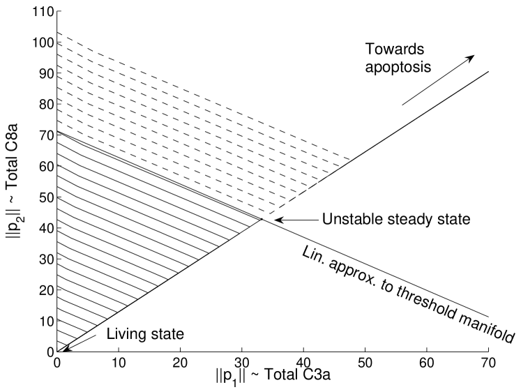
(a) Full model

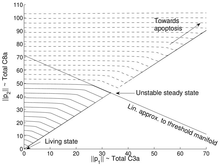
(b) Reduced model

Figure 4: Trajectories of the full and the reduced model projected to a plane spanned by vectors $p_{1}$ and $p_{2}$. These were chosen such that (a) the LATM gets projected to a line and (b) they represent approximately the amount of total C3a and C8a, respectively.

A comparison of the full and the reduced model by numerical simulation yields the results displayed in Fig. 4, obtained by starting with different initial conditions of free C8a. This figure illustrates that the linear approximation to the threshold manifold (LATM) is the same up to projection for both models, as well as the unstable direction of the decision state. Furthermore, the trajectories are very similar when starting close to the decision state.

However, we also observe that the reduced system has different dynamics when considered further away from the decision state. In particular the threshold in initial C8a required to undergo apoptosis is lower in the reduced model. Note that for the full model, the linear threshold displayed in Fig. 4 is a very good approximation of the threshold manifold, while the approximation is not that good for the reduced model. This is likely due to the higher nonlinearities in the reduced model introduced via the steady state maps of the neglected components.

Although the trajectories of the full and the reduced model are different when not starting close to one of the steady states, the results are still meeting our goals, since the focus of our study is more on preserving bistability than recovering a quantitatively similar model. In this way, we have identified a minimal set of components responsible for switch–like behavior.

5 Conclusions

We have studied a mathematical model of a caspase activation system involved in the initiation of apoptosis. The model is bistable to incorporate the switch–like behavior observed in the real system. We have computed the relevance of each state variable to bistability and observed that only four out of eight variables have a high relevance. Using this result, the model can be reduced significantly by retaining only the relevant state variables in the model equations plus the steady state map of the irrelevant variables. The reduced model retains the bistability of the original model and also quantitative features such as trajectories close to the steady states and the linear approximation to the threshold manifold separating the regions of attraction of the two stable steady states.

References

- (1)
- Angeli and Sontag (2004) Angeli, D. and E. D. Sontag (2004). Multi-stability in monotone input/output systems. Syst. Contr. Lett. 51, 185–202.
- Bhattacharyya et al. (1995) Bhattacharyya, S. P., H. Chapellat and L. H. Keel (1995). Robust Control. The parametric approach. Prentice Hall.
- Conzelmann et al. (2004) Conzelmann, H., J. Saez-Rodriguez, T. Sauter, E. Bullinger, F. Allgöwer and E. D. Gilles (2004). Reduction of mathematical models of signal transduction networks: Simulation-based approach applied to egf receptor signaling. IEE Proc. Syst. Biol. 1, 159–169.
- Danial and Korsmeyer (2004) Danial, N. N. and S. J. Korsmeyer (2004). Cell death: critical control points.. Cell 116(2), 205–219.
- Dano et al. (2006) Dano, S., M. F. Madsen, H. Schmidt and G. Cedersund (2006). Reduction of a biochemical model with preservation of its basic dynamic properties. FEBS Journal 273(21), 4862–4877.
- Eißing et al. (2004) Eißing, T., H. Conzelmann, E. D. Gilles, F. Allgöwer, E. Bullinger and P. Scheurich (2004). Bistability analyses of a caspase activation model for receptor-induced apoptosis. J. Biol. Chem. 279(35), 36892–36897.
- Eißing et al. (2007) Eißing, T., S. Waldherr, F. Allgöwer, P. Scheurich and E. Bullinger (2007). Steady state and (bi-) stability evaluation of simple protease signalling networks. BioSystems In Press, –.
- Ferrell and Xiong (2001) Ferrell, James E. and Wen Xiong (2001). Bistability in cell signaling: How to make continuous processes discontinuous, and reversible processes irreversible.. Chaos 11(1), 227–236.
- Pomerening et al. (2003) Pomerening, J. R., E. D. Sontag and J. E. Ferrell (2003). Building a cell cycle oscillator: hysteresis and bistability in the activation of Cdc2.. Nature Cell. Biol. 5(4), 346–351.
- Roussel and Fraser (2001) Roussel, M. R. and S. J. Fraser (2001). Invariant manifold methods for metabolic model reduction. Chaos 11(3), 196–206.
- Schauer and Heinrich (1983) Schauer, M. and R. Heinrich (1983). Quasi-steady-state approximation in the mathematical modeling of biochemical reaction networks. Math. Biosci. 65(2), 155–170.
- Schmidt and Jacobsen (2004) Schmidt, H. and E. W. Jacobsen (2004). Identifying feedback mechanisms behind complex cell behaviour. IEEE Control Syst. Mag. 24, 91–102.
- Schmidt and Jirstrand (2006) Schmidt, H. and M. Jirstrand (2006). Systems Biology Toolbox for Matlab: A computational platform for research in Systems Biology. Bioinformatics 22, 514–515.
- Yildirim et al. (2004) Yildirim, N., M. Santillan, D. Horike and M. C. Mackey (2004). Dynamics and bistability in a reduced model of the lac operon. Chaos 14(2), 279–292.