In search of lost introns

Abstract

Many fundamental questions concerning the emergence and subsequent evolution of eukaryotic exon-intron organization are still unsettled. Genome-scale comparative studies, which can shed light on crucial aspects of eukaryotic evolution, require adequate computational tools.

We describe novel computational methods for studying spliceosomal intron evolution. Our goal is to give a reliable characterization of the dynamics of intron evolution. Our algorithmic innovations address the identification of orthologous introns, and the likelihood-based analysis of intron data. We discuss a compression method for the evaluation of the likelihood function, which is noteworthy for phylogenetic likelihood problems in general. We prove that after $O(n\ell)$ preprocessing time, subsequent evaluations take $O(n\ell/\log\ell)$ time almost surely in the Yule-Harding random model of $n$-taxon phylogenies, where $\ell$ is the input sequence length.

We illustrate the practicality of our methods by compiling and analyzing a data set involving 18 eukaryotes, more than in any other study to date. The study yields the surprising result that ancestral eukaryotes were fairly intron-rich. For example, the bilaterian ancestor is estimated to have had more than 90% as many introns as vertebrates do now.

Contact:

csuros AT iro.umontreal.ca

1 Introduction

Typical eukaryotic protein-coding genes contain introns, which are removed prior to translation. Key constituents of the spliceosome, which is the RNA-protein complex that performs the intron excision, can be traced back CollinsPenny to the last common ancestor of extant eukaryotes (LECA). Even deep-branching lineages introns.trichomonas,introns.giardia have introns. It is thus almost certain that spliceosomal introns were present in LECA. Moreover, when comparing distant eukaryotes, intron positions often agree Rogozin.data. The similarity is likely due more to conservation of early introns than to parallel gains RoyGilbert.earlygenes,Sverdlov.parallelgain. It is thus compelling to use genome-scale comparisons to study intron evolution in different lineages, and even to estimate the exon-intron organization in extinct ancestors. One of the first such studies, by Rogozin.data, involved orthologous gene sets in eight eukaryotes. The same data set was reanalyzed by different authors RoyGilbert.earlygenes,csuros.scenarios,Carmel.EM,Nguyen.introns, using novel methods developed for intron data. Subsequent inquiries introns.fungi,Roy.apicomplexa,Roy.plants,Coulombe.mammals attest to a renewed interest in understanding the specifics of intron evolution within different eukaryotic lineages. This paper introduces novel computational techniques for the analysis of spliceosomal intron evolution, anticipating more large-scale studies to come.

Section 2 describes an alignment method for intron-annotated protein sequences, as well as a segmentation method for identifying conserved portions of a multiple alignment. Section 3 describes a likelihood framework in which intron evolution can be analyzed in a theoretically sound manner. Section 4 scrutinizes a compression technique that accelerates the evaluation of the likelihood function. The compression involves an $O(n\ell)$-time preprocessing step for $\ell$ sites and a phylogeny with $n$ species. We show that the subsequent evaluation takes sublinear, $O(n\ell/\log\ell)$ time almost surely in the Yule-Harding model of random phylogenies, even in the case of arbitrary, constant-size alphabets. Fast evaluation is particularly important when the likelihood is maximized in a numerical procedure that computes the likelihood function with many different parameter settings. Section 5 describes two applications of our methods. In one application, intron-aware alignment was used to validate some unexpected features of intron evolution before LECA. In a second application, we analyzed intron evolution in 18 eukaryotic species. We found evidence of intron-rich early eukaryotes and a prevalence of intron loss over intron gain in recent times.

2 Identification of orthologous introns

2.1 Intron-aware alignment

Orthologous introns can be identified by using whole genome alignments in the case of closely related genomes Coulombe.mammals. For distant eukaryotes, however, intron orthology can only be established through protein alignments Rogozin.methods. The usual procedure is to project intron positions onto an alignment of multiple orthologous proteins. If introns in different species are projected to the same alignment position, then the introns are assumed to be orthologous.

Figure 1: Fragment of a multiple alignment before and after realignment using intron annotation. Shaded rectangles show the intron positions projected to the protein sequences.

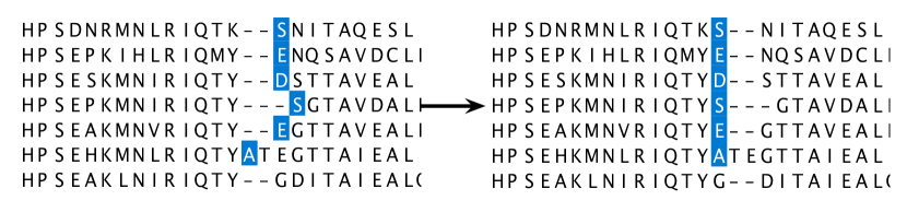
Intron annotation can be included in protein alignments by defining intron match and mismatch scores. The alignment score is then computed as the sum of scores for amino acid matches, gaps, and intron matches. Incorporating intron annotation should lead to better alignments at the amino acid level, and to a more reliable identification of orthologous introns. Figure 1 shows an example of such improvement.

Intron scoring can be based on log-likelihood ratios in a probabilistic model Durbin. The model is defined by the joint distribution $p$ for the intron state in two sequences $S$ and $T$, and the prior distributions $\pi_{S}$ and $\pi_{T}$. Aligned sites have states $(s,t)$ with probability $\pi_{S}(s)\cdot\pi_{T}(t)$ if the two sites are unrelated, or with probability $p(s,t)$ in case of homology. An $(s,t)$ alignment is scored with a value that is proportional to $-\log\frac{p(s,t)}{\pi_{S}(s)\pi_{T}(t)}$.

We used the data set of Rogozin.data to assess the strength of intron-match signals. Since the data include no sites in which all species lack introns, but the model does allow for that, we added extra sites with no introns. The original data comprise 7236 intron sites in 684 genes, across 8 species. Using a method described earlier csuros.scenarios, we added 35000 unobserved intron sites. Using estimates for $p$ and $\pi$, we computed the appropriate scores. The intron score is asymmetric and varies with evolutionary distance and intron conservation. Matches for absent introns have an insignificant score, but shared introns have a high score, such as 93 (human-Plasmodium), 106 (human-Arabidopsis), 152 (human-S. pombe) or 303 (Drosophila-Anopheles) on a 1/60-bit scale. Shared introns thus give a signal comparable to amino acid matches: in the 1/60-bit scaled version of the VTML240 matrix VTML, a tryptophan match scores 289, and an arginine identity scores 113.

Consider the case of aligning two protein sequences, $S$ and $T$, which are annotated with the intron positions. Every residue has two associated intron sites (after the first and second nucleotides of their codons), and there is an intron site between consecutive amino acid positions (phase-0 introns). Intron sites may or may not be filled in by introns in either sequence. We use the notation for ${S}[i\colon 0]$ for the phase-0 site preceding the codon for amino acid $i$, and ${S}[i\colon 1]$, ${S}[i\colon 2]$ for phase-1 and -2 sites within the codon. Intron presence is encoded by 1, and intron absence is encoded by 0 throughout the paper. The intron annotation is specified by the variables ${S}[i\colon j]\in\{\texttt{1},\texttt{0}\}$. (There can be no introns after the last amino acid.) Scores for aligned introns are specified by a $2\times 2$ scoring matrix $\Lambda$.

Phase-1 and phase-2 intron sites are automatically placed by their associated amino acids. If $M$ is the amino acid scoring matrix, then the alignment of $S[i]$ and $T[j]$ entails a score of $M\Big{[}\begin{smallmatrix}{{S}[i]}\\ {{T}[j]}\end{smallmatrix}\Bigr{]}+\Lambda\Bigl{[}\begin{smallmatrix}{{S}[i]}\\ {{T}[j]}\end{smallmatrix}\Bigr{]}$ with $\Lambda\Bigl{[}\begin{smallmatrix}{{S}[i]}\\ {{T}[j]}\end{smallmatrix}\Bigr{]}=\Lambda\Bigl{[}\begin{smallmatrix}{{S}[i\colon 1]}\\ {{T}[j\colon 1]}\end{smallmatrix}\Bigr{]}+\Lambda\Bigl{[}\begin{smallmatrix}{{S}[i\colon 2]}\\ {{T}[j\colon 2]}\end{smallmatrix}\Bigr{]}$. Similarly, aligning $S[i]$ with an indel implies a score of $M\Big{[}\begin{smallmatrix}{{S}[i]}\\ {\texttt{-}}\end{smallmatrix}\Bigr{]}+\Lambda\Bigl{[}\begin{smallmatrix}{{S}[i]}\\ {\texttt{0}}\end{smallmatrix}\Bigr{]}=M\Big{[}\begin{smallmatrix}{{S}[i]}\\ {\texttt{-}}\end{smallmatrix}\Bigr{]}+\Lambda\Bigl{[}\begin{smallmatrix}{{S}[i\colon 1]}\\ {\texttt{0}}\end{smallmatrix}\Bigr{]}+\Lambda\Bigl{[}\begin{smallmatrix}{{S}[i\colon 2]}\\ {\texttt{0}}\end{smallmatrix}\Bigr{]}$, in addition to possible gap opening and closing penalties. Standard alignment procedures need to be modified to deal with phase-0 introns, since the placement of phase-0 introns is not fixed with respect to gaps. It is not possible to simply add a new character to the alphabet to represent phase-0 introns because they affect gaps differently from amino acids.

We added intron scoring into a multiple alignment framework, using a sum-of-pairs scoring policy with affine gap-scoring. It is NP-hard to find the alignment of two multiple alignments under these optimization criteria aliali.NP. Even the alignment of a single sequence to a multiple alignment necessitates sophisticated techniques KececiogluZhang. Our solution therefore uses a gap-counting heuristic: namely, a gap-open penalty is triggered for an indel aligned with an amino acid if the indel is preceded by an amino acid or a phase-0 intron. Gap opening thus corresponds to a pattern $\begin{smallmatrix}\texttt{?x}\\ \texttt{1-}\end{smallmatrix}$ or $\begin{smallmatrix}\texttt{*?x}\\ \texttt{x0-}\end{smallmatrix}$. Here, $\texttt{1},\texttt{0}$ are intron states for the phase-0 site, and ? denotes either state. In addition, x denotes an arbitrary amino acid, - is the indel character, and * is either of the latter two. We implemented affine gap-scoring by separate gap-open and -close penalties, so that gaps at the alignment extremities can be penalized less severely. Gap closing is counted for the patterns $\begin{smallmatrix}\texttt{-1}\\ \texttt{x?}\end{smallmatrix}$ and $\begin{smallmatrix}\texttt{-0x}\\ \texttt{x?*}\end{smallmatrix}$.

Table 1 gives the recurrences for a dynamic programming algorithm that aligns an intron-annotated sequence $S$ to a multiple alignment $P$ of $h$ intron-annotated protein sequences. In order to simplify the presentation, we represent the sequences in such a way that every odd position of $S$ and $P$ is a regular residue or alignment column, annotated with information on the presence of phase-1 and phase-2 introns, whereas every even position is a phase-0 intron site. We use $\Lambda\Bigl{[}\begin{smallmatrix}{{S}[i]}\\ {{P}[j]}\end{smallmatrix}\Bigr{]}$ to denote the sum of intron-match scores for the intron sites associated with the positions $S[i]$, $P[j]$. We use also the shorthand $M\Big{[}\begin{smallmatrix}{x}\\ {\mathbf{y}}\end{smallmatrix}\Bigr{]}$ to denote scoring for the alignment of an amino acid $x$ with an amino acid profile $\mathbf{y}$. The algorithm uses three types of variables, $\mathsf{A}[i,j]$, $\mathsf{gS}[i,j]$ and $\mathsf{gP}[i,j]$, which correspond to partial prefix alignments ending with aligned residues, gaps in $S$, or gaps in $P$, respectively. In case of $\mathsf{gS}[i,j]$, the last indel must be aligned with an amino acid column, and, thus $j$ must be odd; for $\mathsf{gP}[i,j]$, $i$ must be odd.

$$\mathsf{A}[i,j] =\begin{aligned} &M\Big{[}\begin{smallmatrix}{{S}[i]}\\ {{P}[j]}\end{smallmatrix}\Bigr{]}+\Lambda\Bigl{[}\begin{smallmatrix}{{S}[i]}\\ {{P}[j]}\end{smallmatrix}\Bigr{]}+\gamma^{(-)}_{1}(j)+\max\Bigl{\{}\mathsf{A}[i-2,j-2]+\Lambda\Bigl{[}\begin{smallmatrix}{{S}[i-1]}\\ {{P}[j-1]}\end{smallmatrix}\Bigr{]}+\gamma^{(<)}_{1}(j)+\gamma^{(>)}_{1}(j),\\ &\mathsf{gS}[i-2,j-2]+\Lambda\Bigl{[}\begin{smallmatrix}{{S}[i-1]}\\ {{P}[j-1]}\end{smallmatrix}\Bigr{]}+\gamma^{(<)}_{1}(j)+\gamma^{(>)}_{2}(j-2),\mathsf{gS}[i-1,j-2]+\Lambda\Bigl{[}\begin{smallmatrix}{\texttt{0}}\\ {{P}[j-1]}\end{smallmatrix}\Bigr{]}+\gamma^{(<)}_{1}(j)+\gamma^{(>)}_{2}(j-2),\\ &\mathsf{gP}[i-2,j-2]+\Lambda\Bigl{[}\begin{smallmatrix}{{S}[i-1]}\\ {{P}[j-1]}\end{smallmatrix}\Bigr{]}+\gamma^{(<)}_{2}(j)+\gamma^{(>)}_{3}(j),\mathsf{gP}[i-2,j-1]+\Lambda\Bigl{[}\begin{smallmatrix}{{S}[i-1]}\\ {\texttt{0}^{h}}\end{smallmatrix}\Bigr{]}+\gamma^{(>)}_{2}(j)\Bigr{\}}\end{aligned} i j$$ odd , odd

$$\mathsf{gS}[i,j] =\begin{aligned} &\Lambda\Bigl{[}\begin{smallmatrix}{\texttt{0}}\\ {{P}[j]}\end{smallmatrix}\Bigr{]}+\gamma^{(-)}_{2}(j)+\max\Bigl{\{}\mathsf{A}[i,j-2]+\Lambda\Bigl{[}\begin{smallmatrix}{\texttt{0}}\\ {{P}[j-1]}\end{smallmatrix}\Bigr{]}+\gamma^{(<)}_{3}(j)+\gamma^{(>)}_{1}(j),\\ &\mathsf{gS}[i,j-2]+\Lambda\Bigl{[}\begin{smallmatrix}{\texttt{0}}\\ {{P}[j-1]}\end{smallmatrix}\Bigr{]},\\ &\mathsf{gP}[i,j-2]+\Lambda\Bigl{[}\begin{smallmatrix}{\texttt{0}}\\ {{P}[j-1]}\end{smallmatrix}\Bigr{]}+\gamma^{(<)}_{3}(j)+\gamma^{(>)}_{3}(j),\mathsf{gP}[i,j-1]+\Lambda\Bigl{[}\begin{smallmatrix}{\texttt{0}}\\ {\texttt{0}^{h}}\end{smallmatrix}\Bigr{]}+\gamma^{(<)}_{3}(j)+\gamma^{(>)}_{2}(j)\Bigr{\}}\end{aligned} i j$$ odd , odd

$$\mathsf{gP}[i,j] =\begin{aligned} &\Lambda\Bigl{[}\begin{smallmatrix}{{S}[i]}\\ {\texttt{0}^{h}}\end{smallmatrix}\Bigr{]}+\gamma^{(-)}_{1}(j)+\max\Bigl{\{}\mathsf{A}[i-2,j]+\Lambda\Bigl{[}\begin{smallmatrix}{{S}[i-1]}\\ {\texttt{0}^{h}}\end{smallmatrix}\Bigr{]}+\gamma^{(<)}_{3}(j),\\ &\mathsf{gS}[i-2,j]+\Lambda\Bigl{[}\begin{smallmatrix}{{S}[i-1]}\\ {\texttt{0}^{h}}\end{smallmatrix}\Bigr{]}+\gamma^{(<)}_{3}(j)+\gamma^{(>)}_{2}(j),\mathsf{gS}[i-1,j]+\Lambda\Bigl{[}\begin{smallmatrix}{\texttt{0}}\\ {\texttt{0}^{h}}\end{smallmatrix}\Bigr{]}+\gamma^{(<)}_{3}(j)+\gamma^{(>)}_{2}(j),\\ &\mathsf{gP}[i-2,j]+\Lambda\Bigl{[}\begin{smallmatrix}{{S}[i-1]}\\ {\texttt{0}^{h}}\end{smallmatrix}\Bigr{]}\Bigr{\}}\end{aligned} i j$$ odd , odd

$$\mathsf{gS}[i,j] =\begin{aligned} &\Lambda\Bigl{[}\begin{smallmatrix}{\texttt{0}}\\ {{P}[j]}\end{smallmatrix}\Bigr{]}+\gamma^{(-)}_{2}(j)+\max\Bigl{\{}\mathsf{A}[i-1,j-2]+\Lambda\Bigl{[}\begin{smallmatrix}{{S}[i]}\\ {{P}[j-1]}\end{smallmatrix}\Bigr{]}+\gamma^{(<)}_{3}(j)+\gamma^{(>)}_{1}(j),\\ &\mathsf{gS}[i-1,j-2]+\Lambda\Bigl{[}\begin{smallmatrix}{{S}[i]}\\ {{P}[j-1]}\end{smallmatrix}\Bigr{]}+\gamma^{(<)}_{4}(i,j)+\gamma^{(>)}_{4}(i,j),\mathsf{gS}[i,j-2]+\Lambda\Bigl{[}\begin{smallmatrix}{\texttt{0}}\\ {{P}[j-1]}\end{smallmatrix}\Bigr{]},\\ &\mathsf{gP}[i-1,j-2]+\Lambda\Bigl{[}\begin{smallmatrix}{{S}[i]}\\ {{P}[j-1]}\end{smallmatrix}\Bigr{]}+\gamma^{(<)}_{3}(j)+\gamma^{(>)}_{3}(j),\mathsf{gP}[i-1,j-1]+\Lambda\Bigl{[}\begin{smallmatrix}{{S}[i]}\\ {\texttt{0}^{h}}\end{smallmatrix}\Bigr{]}+\gamma^{(<)}_{3}(j)+\gamma^{(>)}_{2}(j)\Bigr{\}}\end{aligned} i j$$ even , odd

$$\mathsf{gP}[i,j] =\begin{aligned} &\Lambda\Bigl{[}\begin{smallmatrix}{{S}[i]}\\ {\texttt{0}^{h}}\end{smallmatrix}\Bigr{]}+\gamma^{(-)}_{1}(j)+\max\Bigl{\{}\mathsf{A}[i-2,j-1]+\Lambda\Bigl{[}\begin{smallmatrix}{{S}[i-1]}\\ {{P}[j]}\end{smallmatrix}\Bigr{]}+\gamma^{(<)}_{5}(j)+\gamma^{(>)}_{5}(j),\\ &\mathsf{gS}[i-2,j-1]+\Lambda\Bigl{[}\begin{smallmatrix}{{S}[i-1]}\\ {{P}[j]}\end{smallmatrix}\Bigr{]}+\gamma^{(<)}_{5}(j)+\gamma^{(>)}_{2}(j-1),\mathsf{gS}[i-1,j-1]+\Lambda\Bigl{[}\begin{smallmatrix}{\texttt{0}}\\ {{P}[j]}\end{smallmatrix}\Bigr{]}+\gamma^{(<)}_{5}(j)+\gamma^{(>)}_{2}(j-1),\\ &\mathsf{gP}[i-2,j-1]+\Lambda\Bigl{[}\begin{smallmatrix}{{S}[i-1]}\\ {{P}[j]}\end{smallmatrix}\Bigr{]}+\gamma^{(<)}_{6}(j)+\gamma^{(>)}_{6}(j),\mathsf{gP}[i-2,j]+\Lambda\Bigl{[}\begin{smallmatrix}{{S}[i-1]}\\ {\texttt{0}^{h}}\end{smallmatrix}\Bigr{]}\Bigr{\}}\end{aligned} i j$$ odd , even

Table 1: Recurrences for intron-aware alignment. Odd positions correspond to regular amino acids and possibly phase-1 and -2 introns. Even positions are placeholders for phase-0 intron sites.

Gaps are scored by using affine penalties, with gap-open, -extend, and -close scores, denoted by $\gamma^{(<)},\gamma^{(-)},\gamma^{(>)}$. The gap-counting heuristic implies that gap scores in the equations of Table 1 are defined by the number of certain patterns in up to three consecutive alignment columns. For instance, $\gamma^{(<)}_{2}(j)$ equals the gap-open penalty multiplied by the number of such rows in $P$ where column $j$ contains an indel, and column $j-1$ has a phase-0 intron. The corresponding pattern is described as 1-. Table 2 lists the patterns for the gap-counting heuristic.

$$\begin{array}[]{llllll}\gamma^{(<)}_{1}&\texttt{1}\texttt{-}\text{ or }\texttt{x}\texttt{0}\texttt{-}&\gamma^{(<)}_{2}&\texttt{1}\texttt{-}\\ \gamma^{(<)}_{3}&\texttt{x}&\gamma^{(<)}_{4}&\texttt{x}\text{ if ${S}[i]$ has intron, otherwise nothing}\\ \gamma^{(<)}_{5}&\texttt{1}\text{ or }\texttt{x}\texttt{0}&\gamma^{(<)}_{6}&\texttt{1}\\ \gamma^{(>)}_{1}&\texttt{-}\texttt{0}\texttt{x}\text{ or }\texttt{-}\texttt{1}\texttt{*}&\gamma^{(>)}_{2}&\texttt{x}\\ \gamma^{(>)}_{3}&\texttt{1}\texttt{*}\text{ or }\texttt{0}\texttt{x}&\gamma^{(>)}_{4}&\texttt{x}\text{ if ${S}[i]$ has intron, otherwise nothing}\\ \gamma^{(>)}_{5}&\texttt{-}\texttt{1}&\gamma^{(>)}_{6}&\texttt{1}\\ \gamma^{(-)}_{1}&\texttt{-}&\gamma^{(-)}_{2}&\texttt{x}\end{array}$$

Table 2: Patterns for gap counting. The index $j$ in $\gamma^{(<)}(j)$, $\gamma^{(-)}(j)$ and $\gamma^{(>)}(j)$ is the index for the last column in the pattern.

Table 1 does not show the initialization of the variables, nor the final gap-counting: they employ a logic analogous to the recurrences. At the end of the algorithm, the best of $\mathsf{A}[|S|,|P|]$, $\mathsf{gS}[|S|,|P|]$, $\mathsf{gP}[|S|,|P|]$ is selected, and the actual alignment is found by standard traceback techniques Durbin.

We implemented the algorithm in Java. The program iteratively realigns one sequence at a time to the rest of the sequences in a multiple alignment. Instead of sequence-dependent intron match-mismatch scores, the implementation uses only two parameters: one for intron conservation and another for intron loss/gain.

2.2 Identification of conserved blocks

In order to reliably identify orthologs, we need to be able to distinguish regions of the alignment that are highly conserved from those that are less well-conserved. In poorly conserved regions, we cannot confidently infer intron orthology.

postprocessing proposed post-processing pairwise sequence alignments into alternating blocks that score above a threshold parameter $\alpha$ or below $(-\alpha)$. We attained a similar goal by adapting algorithmic technniques from segment-sets. The procedure separates a multiple alignment into alternating high- and low-scoring regions. Using a complexity penalty $\alpha$, a segmentation with $k$ high-scoring regions has a segmentation score of $A-k\alpha$ where $A$ is the sum of scores for the aligned columns. Column scores are computed without gap-open and -close penalties. The best segmentation of an alignment of length $\ell$ can be found in $O(\ell)$ time after the column scores are computed.

The result of this computation is that the total of column scores in each selected high-scoring region will be greater than $\alpha$. There may be small sub-regions of negative scores, but the total score of such a sub-region cannot be less than $(-\alpha)$. Conversely, unselected regions score below $(-\alpha)$ and cannot have sub-regions scoring above $\alpha$.

3 A likelihood framework

3.1 Markov models of evolution

We use a Markov model for intron evolution, as in previous studies csuros.scenarios. For the sake of generality, we describe the Markov model Steel.markov,Felsenstein over an arbitrary alphabet $\mathcal{A}$ of fixed size $r=|\mathcal{A}|$. The intron alphabet is $\mathcal{A}=\{\texttt{0},\texttt{1}\}$. A phylogeny over a set of species $X$ is defined by a rooted tree $T$ and a probabilistic model. The leaves are bijectively mapped to elements of $X$. Each tree node $u$ has an associated random variable $\xi(u)$, which is called its state or label, that takes values over $\mathcal{A}$. The tree $T$ with its parameters defines the joint distribution for the random variables $\xi(u)$. The distribution is determined by the root probabilities $\bigl{(}\pi(a)\colon a\in\mathcal{A}\bigr{)}$ and edge transition probabilities $\bigl{(}p_{e}(a\rightarrow b)\colon a,b\in\mathcal{A}\bigr{)}$ assigned to every edge $e$. The root probabilities give the distributon of the root state. Edge transition probabilities define the conditional distributions ${\mathbb{P}}\Bigl{\{}\xi(u_{i+1})=b\Bigm{|}\xi(u_{i})=a\Bigr{\}}=p_{u_{i}u_{i+1}}(a\rightarrow b)$. Along every path away from the root, the node states form a Markov chain. The leaf states form the character $\xi=(\xi(u)\colon u\in X)$. An input data set (or sample) consists of independent and identically distributed (iid) characters: $\boldsymbol{\xi}=(\xi_{i}\colon i=1,\ldots,\ell)$.

In case of intron evolution, introns are generated by a two-state continuous-time Markov process with gain and loss rates $\lambda_{e},\mu_{e}\geq 0$ along each edge $e$. The edge length is denoted by $t_{e}$. Using standard results Ross, the transition probabilities on edge $e$ with rates $\lambda_{e}=\lambda,\mu_{e}=\mu$ and length $t_{e}=t$ can be written as $p_{e}(\texttt{0}\rightarrow\texttt{1})=\frac{\lambda}{\lambda+\mu}\bigl{(}1-e^{-t(\lambda+\mu)}\bigr{)}$, $p_{e}(\texttt{1}\rightarrow\texttt{0})=\frac{\mu}{\lambda+\mu}\bigl{(}1-e^{-t(\lambda+\mu)}\bigr{)}$, and $p_{e}(\texttt{0}\rightarrow\texttt{0})=1-p_{e}(\texttt{0}\rightarrow\texttt{1})$, $p_{e}(\texttt{1}\rightarrow\texttt{1})=1-p_{e}(\texttt{1}\rightarrow\texttt{0})$. In the absence of established edge lengths, we fix the edge length scaling in such a way that $\lambda_{e}+\mu_{e}=1$. Independent model parameters are thus $\pi(\texttt{1})$, $\nu_{e}$ and $t_{e}$ for all edges $e$. It is important to allow for branch-dependent rates, since loss and gain rates vary considerably between lineages Jeffares.gainloss,RoyGilbert.review.

In a maximum likelihood approach, model parameters are set by maximizing the likelihood of the input sample. Let $\mathbf{x}=(x_{1},\dotsc,x_{\ell})$ be the input data. Every $x_{i}$ is a vector of $n$ states, and we write $x_{i}(u)$ to denote the observed state of leaf $u$. By independence, the likelihood of $\mathbf{x}$ is the product $\mathbb{P}\{\boldsymbol{\xi}=\mathbf{x}\}=\prod_{i}\mathbb{P}\{\xi=x_{i}\}$. Each character’s likelihood can be computed in $O(n)$ time, using a dynamic programming procedure introduced by Felsenstein.ML. The procedure relies on a “pruning” technique, which consists of computing the conditional likelihoods $L_{u}(a)$ for every node $u$ and letter $a$. $L_{u}(a)$ is the probability of observing the leaf labelings in the subtree of $u$, given that $u$ is labeled with $a$. The likelihood for the character $x$ equals $L(x)=\mathbb{P}\{\xi=x\}=\sum_{a\in\mathcal{A}}\pi(a)L_{\mathsf{root}}(a)$.

Intron data are somewhat unusual in that an all-0 character is never observed: the input does not include sites in which introns are absent in all of the organisms. The uncorrected likelihood function is therefore misleading, as it underestimates the probability of intron loss. To resolve this difficulty, we employ a correction technique proposed by Felsenstein.restml for restriction sites. (csuros.scenarios describes an alternative technique based on expectation maximization.) We compute the likelihood under the condition that the input does not include all-0 characters. We use therefore the corrected likelihood $L^{\prime}(x)=\frac{L(x)}{1-L(\texttt{0}^{n})}$, and maximize $L^{\prime}=\prod_{i}L^{\prime}(x_{i})$.

3.2 Ancestral events in intron evolution

Our goal is to give a reliable characterization of the dynamics of intron evolution. In particular, we aim to give estimates for intron density in ancestral species, and for intron loss and gain events on the edges. Notice that the estimation method needs to account for ancestral introns even if they got eliminated in all descendant lineages. It is possible to do that with the help of conditional expectations, which fit naturally into a likelihood framework.

For an observed character $x$, we define upper conditional likelihoods $U_{u}(a)$ so that $U_{u}(a)L_{u}(a)=\mathbb{P}\{\xi=x,\xi(u)=a\}$. Upper conditional likelihoods are computed with dynamic programming, from the root towards the leaves, in $O(n\ell)$ time csuros.scenarios, even for non-binary trees. Similar computations are routinely used in DNA and protein likelihood maximization programs MOLPHY,PhyML. Here we allow irreversible probabilistic models, which explains why $U_{u}(a)$ must be computed in a top-down fashion in (1).

The posterior probability for the state at node $u$ is

$$q_{a}^{(u)}(x)={\mathbb{P}}\Bigl{\{}\xi(u)=a\Bigm{|}\xi=x\Bigr{\}}=\frac{U_{u}(a)L_{u}(a)}{\sum_{b\in\mathcal{A}}U_{u}(b)L_{u}(b)}.$$

The posterior probabilities for state changes on an edge $uv$ are

$$q_{ab}^{(v)}(x)={\mathbb{P}}\Bigl{\{}\xi(u)=a,\xi(v)=b\Bigm{|}\xi=x\Bigr{\}}\\ =U_{u}(a)L_{u}(a)\frac{p_{uv}(a\rightarrow b)L_{v}(b)}{\sum_{a^{\prime}}p_{uv}(a\rightarrow a^{\prime})L_{v}(a^{\prime})}.$$

Now, the number of ancestral introns is estimated as the conditional expectation $N_{u}=\ell_{0}q_{\texttt{1}}^{(u)}(\texttt{0}^{n})+\sum_{i}q_{\texttt{1}}^{(u)}(x_{i})$. The formula takes into consideration unobserved intron sites, by estimating their number $\ell_{0}=\ell\frac{L(\texttt{0}^{n})}{1-L(\texttt{0}^{n})}$ as the mean of a negative binomial random variable. The number of intron state changes is estimated as $N_{v}(a\rightarrow b)=\ell_{0}q_{ab}^{(v)}(\texttt{0}^{n})+\sum_{i}q_{ab}^{(v)}(x_{i})$. In particular, $N_{v}(\texttt{1}\rightarrow\texttt{0})$ is the number of introns lost, and $N_{v}(\texttt{0}\rightarrow\texttt{1})$ is the number of introns gained on the edge leading to $v$.

In order to compute $U$, we initialize $U_{\mathsf{root}}(a)=\pi(a)$. On every edge $uv$,

$$U_{v}(b)\\ =\sum_{a\in\mathcal{A}}U_{u}(a)p_{uv}(a\rightarrow b)\prod_{w\in\mathsf{siblings}(v)}\sum_{a^{\prime}\in\mathcal{A}}p_{uw}(a\rightarrow a^{\prime})L_{w}(a^{\prime})\\ =\sum_{a\in\mathcal{A}}U_{u}(a)L_{u}(a)\frac{p_{uv}(a\rightarrow b)L_{v}(b)}{\sum_{a^{\prime}\in\mathcal{A}}p_{uv}(a\rightarrow a^{\prime})L_{v}(a^{\prime})}.$$ (1)

4 Rapid computation of the likelihood

There are many heuristics that accelerate likelihood-based phylogenetic reconstruction SEMPHY,PhyML, which mostly concentrate on the exploration of the tree space. We propose an improvement to the evaluation of the likelihood function, which normally takes linear time in the input size. Our evaluation method yields an $O(\log\ell)$ speedup for typical trees. We use it to optimize the parameters of intron evolution on a known tree, but the method is generally applicable to phylogenetic likelihood problems where the likelihood is numerically optimized. The key idea is that it is enough to carry out the pruning algorithm once for every different labeling within a subtree. Different labelings within each subtree can be computed in a preprocessing step. Subsequent evaluations of the likelihood function with different model parameters are faster, and depend on the number of different labelings in the data set.

Here we describe how the preprocessing step can be carried out in $O(n\ell)$ time. Secondly, we analyze the computational complexity of subsequent evaluations, and show that an $O(\log\ell)$ speedup is achieved for almost all random trees in the Yule-Harding model. The latter analysis produces some novel concentration results on the number of subtrees with a fixed size $k$.

To our knowledge, the closest idea to ours was articulated by AxML. Specifically, they proposed identifying characters in which leaves in a subtree have identical labels. They reported that in benchmark experiments with nucleotide sequences, likelihood optimization was accelerated by 12–15% through this technique. The technique relies entirely on the fact that alignments of closely related sequences exhibit high levels of identity, and cannot be extended to non-identical labelings.

4.1 Yule-Harding model

The Yule-Harding distribution is encountered in random birth and death models of species and in coalescent models Felsenstein, and is thus one of the most adequate random models for phylogenies. In one of the equivalent formulations, a random tree is grown by adding leaves one by one in a random order. The leaves are first numbered by using a random uniform permutation of the integers $1,2,\dotsc,n$. Leaves are joined to the tree in an iterative procedure. In step 1, the tree is just leaf 1 on its own. In step 2, the tree is a “cherry” with leaves $1$ and $2$. In each subsequent step $i=3,\dotsc,n$, a random leaf $Y_{i}$ is picked uniformly from the set $\{1,2,\dotsc,i-1\}$. The new leaf $i$ is added to the tree as the sibling of $Y_{i}$, forming a cherry: a new node is placed on the edge leading to $Y_{i}$ and $i$ is connected to it. The resulting random tree in iteration $n$ has the Yule-Harding distribution Harding.

Algorithm Compress C1 for every leaf $u$ do C2 initialize $a[1..r]\leftarrow 0$ // $a[j]$ is the first occurrence of state $j$ C3 for $i\leftarrow 1,\dotsc,\ell$ do C4 if $a[x_{i}(u)]=0$ then $a[x_{i}(u)]\leftarrow i$ C5 set $h_{i}(u)\leftarrow a[x_{i}(u)]$ C6 for every non-leaf node $u$ in a post-order traversal do C7 initialize the map $H\colon\{1,\dotsc,\ell\}^{2}\mapsto\{1,\dotsc,\ell\}$ as empty C8 let $v,w$ be the left and right children of $u$ C9 for $i\leftarrow 1,\dotsc,\ell$ do C10 if $H(h_{i}(v),h_{i}(w))=\mathsf{null}$ then $H(h_{i}(v),h_{i}(w))\leftarrow i$ C11 set $h_{i}(u)\leftarrow H(h_{i}(v),h_{i}(w))$

Figure 2: Computing the auxiliary arrays from which the multiplicities $\nu_{u}$ are obtained.

4.2 Preprocessing

The likelihood can be computed faster by first identifying the different $x_{i}$ values, along with their multiplicity in the data. For large trees, the input typically consists of many different labelings, but for small trees with $n<\log_{r}\ell)$, the compression is useful, since the number of different $x_{i}$ values is bounded by $r^{n}<\ell$. In order to exploit the benefits of compression, we extend it to every subtree.

Definition 1.

Define the multiset of observed labelings for every node $u$ as follows. Let $n^{\prime}$ denote the number of leaves in the subtree rooted at $u$, and let $u_{1},\dotsc,u_{n^{\prime}}$ denote those leaves. Define $\nu_{u}(y)$ for every labeling $y\in\mathcal{A}^{n^{\prime}}$ of the leaves in the subtree of $u$ as the number of times $y$ is observed in the data:

$$\nu_{u}(y)=\sum_{i=1}^{\ell}\chi\Bigl{\{}\forall\,k\colon y_{k}=x_{i}(u_{k})\Bigr{\}},$$

where $\chi\{\cdot\}$ denotes the indicator function that takes the value 1 if its argument is true, otherwise it is 0. Define also the set of observed labelings

$$\mathcal{S}_{u}=\Bigl{\{}y\in\mathcal{A}^{n^{\prime}}\colon\nu_{u}(y)>0\Bigr{\}}.$$

The multisets of observed labelings are computed in the preprocessing step. The likelihood function is evaluated subsequently by computing the conditional likelihoods at each node $u$ for the labelings of $\mathcal{S}_{u}$ only, in $O(|\mathcal{S}_{u}|)$ time.

In order to compute $\nu_{u}$, we use a recursive procedure. It is important to avoid working with the $O(n)$-dimensional vectors $y$ of Definition 1 directly, otherwise the preprocessing may take superlinear time in $n$. For that reason, every labeling $y\in\mathcal{S}_{u}$ is represented by the index $i$ for which $x_{i}$ is the first occurrence of $y$. Accordingly, we compute an auxiliary array $h_{i}(u)$, which stores the first occurrence of each labeling $x_{i}$ in $u$’s subtree. In particular, $h_{i}(u)=i^{\prime}$ if $i^{\prime}$ is the smallest index such that $x_{i}(u_{k})=x_{i^{\prime}}(u_{k})$ for all $k$ where $u_{k}$ are the leaves in $u$’s subtree. Figure 2 shows that the values $h_{i}(u)$ can be computed in a post-order traversal. After $h_{i}(u)$ are computed for all $i$ and $u$, the multiplicities $\nu_{u}$ and observed labelings $\mathcal{S}_{u}$ are straightforward to calculate in linear time. The map $H$ in Lines C7–C11 is sparse with at most $\ell$ entries, and can be implemented as a hash table so that accessing and updating it takes $O(1)$ time. Consequently, Algorithm Compress takes $O(n\ell)$ time.

Algorithm LogLikelihood L1 for every leaf $u$ do L2 set $L_{u}[a][a^{\prime}]\leftarrow\chi\{a=a^{\prime}\}$ for all $a\in\mathcal{S}_{u}$ and $a^{\prime}\in\mathcal{\mathcal{A}}$ L3 for every non-leaf node $u$ in a post-order traversal do L4 for every labeling $y\in\mathcal{S}_{u}$ do L5 let $u_{1},u_{2}$ be the children of $u$, and let $y_{1},y_{2}$ be their subtree labelings L6 for every $a\in\mathcal{A}$ L7 $L_{u}[y][a]\leftarrow\prod_{j=1,2}\sum_{a^{\prime}\in\mathcal{A}}p_{uu_{j}}(a\rightarrow a^{\prime})L_{u_{j}}[y_{j}][a^{\prime}]$ L8 set $\mathsf{logL}\leftarrow 0$ L9 for every labeling $y\in\mathcal{S}_{\mathsf{root}}$ do L10 $\mathsf{logL}\leftarrow\mathsf{logL}+\nu_{\mathsf{root}}(y)\cdot\sum_{a\in\mathcal{A}}\log\bigl{(}\pi(a)L_{\mathsf{root}}[y][a]\bigr{)}$ L11 return $\mathsf{logL}$

Figure 3: Computing the log-likelihood using the observed labelings.

4.3 Evaluating the likelihood function

After the preprocessing step, the conditional likelihoods are computed only for the different labelings within each subtree. Figure 3 shows the evaluation of the likelihood function. The running time for the algorithm is $O(s)$ where $s$ is the total number of different labelings within all subtrees:

$$s=\sum_{u}|\mathcal{S}_{u}|.$$

If $n_{u}$ denotes the number of leaves in the subtree rooted at $u$, then $\mathcal{S}_{u}$ has at most $r^{n_{u}}$ elements. Hence, $s$ is bounded as

$$s\leq\sum_{u}\min\{r^{n_{u}},\ell\}.$$ (2)

Observe that by sheer number of arithmetic operations, it is always worth evaluating the likelihood function this way. The worst situation is that of a caterpillar tree (where every inner node has a leaf child). In that case, there are only a few ($\lfloor\log_{r}\ell\rfloor-1$) non-leaf nodes for which we can compress the data, and it is possible to construct an artificial data set in which there are $\ell$ different labelings for $n-O(\log\ell)$ subtrees. Caterpillar trees, however, are rare in phylogenetic analysis. Typical phylogenies have fairly balanced subtrees Aldous.beta.

In what follows, we examine the bound of (2) more closely in the Yule-Harding model. The analysis relies on a characterization of the random number of subtrees with a given size, as expressed in Theorems 1 and 2.

Theorem 1.

Consider random evolutionary trees with $n$ leaves in the Yule-Harding model. Let $C_{k}$ denote the number of subtrees with $k=1,\dotsc,n-1$ leaves in a random tree. The expected value of $C_{k}$ is

$$\mathbb{E}C_{k}=2n\Bigl{(}\frac{1}{k}-\frac{1}{k+1}\Bigr{)}.$$ (3)

Trivially, $\mathbb{E}C_{n}=1$.

Proof.

Heard.subtrees derives Equation (3) by appealing to a Pólya urn model. An equivalent result is stated by Devroye.subtrees.normal.

$\Box$∎

Theorem 2.

For all $\epsilon>0$,

$$\mathbb{P}\bigl{\{}C_{k}\leq\mathbb{E}C_{k}-\epsilon\bigr{\}} \leq e^{-\frac{\epsilon^{2}}{2n}};$$ (4a)

$$\mathbb{P}\bigl{\{}C_{k}\geq\mathbb{E}C_{k}+\epsilon\bigr{\}} \leq e^{-\frac{\epsilon^{2}}{2n}}.$$ (4b)

Proof.

Consider the random construction of the tree. Let $Y_{i}$ denote the random leaf picked in step $i$ to which leaf $i$ gets connected, for $i=3,4,\dotsc,n$. Each random variable $Y_{i}$ is uniformly distributed over the set $\{1,2,\dotsc,i-1\}$, and $Y_{3},Y_{4},\dotsc,Y_{n}$ are independent. Moreover, they completely determine the tree $T$ at the end of the procedure. Consequently, $C_{k}$ is a function of $(Y_{i}\colon i=3,\dotsc,n)$: $C_{k}=f(Y_{3},Y_{4},\dotsc,Y_{n})$. The key observation for the concentration result is that if we change the value of only one of the $Y_{i}$ in the series, then $C_{k}$ changes by at most two. In order to see this, consider what happens to the tree $T$, if we change the value of exactly one of the $Y_{i}$ from $y$ to $y^{\prime}$. Such a change corresponds to a “subtree prune and regraft” transformation Felsenstein. Specifically, the subtree $T_{i}$, defined as the child tree of the lowest common ancestor $u$ of $y$ and $i$ containing the leaf $i$, is cut from $T$, and is reattached to one of the edges on the path from the root to $y^{\prime}$. Now, such a transformation does not affect $C_{k}$ by much. Notice that subtree sizes are strictly monotone decreasing from the root on every path. On the path from the root to $u$, subtree sizes decrease by the size $\tau$ of $T_{i}$, and $u$ disappears, contributing a change of $+1$, $0$ or $(-1)$ to $C_{k}$. (At most one subtree of size $\tau+k$ that contains $T_{i}$ now has size $k$, and at most one subtree of original size $k$ is not counted anymore: it may be $u$’s subtree itself, or a subtree above it.) An analogous argument shows that regrafting contributes a change of $+1$, $0$, or $(-1)$. Hence, the function $f(\cdot)$ is such that by changing one of its arguments, its value changes by at most $2$. As a consequence, McDiarmid’s inequality (McDiarmid) can be applied to bound the probabilities of large deviations for $C_{k}$. In particular, for all $\epsilon>0$,

$$\mathbb{P}\bigl{\{}f(Y_{3},\dotsc,Y_{n})-\mathbb{E}f(Y_{3},\dotsc,Y_{n})\leq-\epsilon\bigr{\}}\leq e^{-2\epsilon^{2}/c^{2}}$$

where $c^{2}=\sum_{i=3}^{n}c_{i}^{2}$ and

$$c_{i}=\max_{y_{3},\dotsc,y_{n},y,y^{\prime}}\Bigl{|}f(y_{3},\dotsc,y_{i-1},y,y_{i+1},\dotsc,y_{n})\\ -f(y_{3},\dotsc,y_{i-1},y^{\prime},y_{i+1},\dotsc,y_{n})\Bigr{|}.$$

Since $c_{i}\leq 2$ for all $i$, $\mathbb{P}\bigl{\{}C_{k}\leq\mathbb{E}C_{k}-\epsilon\bigr{\}}\leq e^{-\frac{\epsilon^{2}}{2(n-2)}}$, implying Eq. (4a). An identical bound holds for the right-hand tail of the distribution. $\Box$∎

Remark.  The particular case of $k=2$ was considered by McKenzieSteel.cherries. They showed that the distribution of $C_{2}$ is asymptotically normal with mean $n/3$ and variance $2n/45$. The result suggests that the best constant factor in the exponent of Eqs. (4) is $45/8$ for $i=2$, instead of $\frac{1}{2}$. Rosenberg.subtrees gave exact formulas for the variance of $C_{k}$. He showed that the variance of $C_{k}$ is $(2+o(1))\frac{n}{k^{2}}$. The variance formulas were given earlier in a different context by Devroye.subtrees.normal. (See also the discussion by BlumFrancois.Sackin.) The result suggests that by analogy with the cherries, the best constant factor in the exponent is $(1/4+o(1))k^{2}$. It is thus plausible that the probability is properly bounded by $1-o\bigl{(}n\log^{-2}\ell\bigr{)}$ in Theorem 3 below.

Theorem 3.

With probability $1-o\Bigl{(}\frac{n}{\log^{4}\ell}\Bigr{)}$, the likelihood function can be evaluated for random trees in the Yule-Harding model in $O\Bigl{(}\frac{n\ell}{\log\ell}\Bigr{)}$ time after an initial preprocessing step that takes $O(n\ell)$ time. Evaluating the likelihood function takes $O(n\ell)$ time in the worst case, and $O(n\ell\log^{-1}\ell)$ time on average.

We need the following lemma for the proof of Theorem 3.

Lemma 4.

For all $t\geq 4$, $\sum_{k=1}^{t}\frac{2^{k}}{k(k+1)}<\frac{2^{t}}{t+1}$. For all $t\geq 1$ and $r=3,4,\dotsc$, $\sum_{k=1}^{t}\frac{r^{k}}{k(k+1)}\leq\frac{r^{t}}{t+1}$.

Proof.

The proof is straightforward by induction in $t$. Notice that the right order of magnitude is $\sum_{k=1}^{t}\frac{r^{k}}{k(k+1)}=\Theta\bigl{(}t^{-2}r^{t}\bigr{)}$ but we need a bound for all $t$. $\Box$∎

$n$	$\ell$	$r$	$n\ell$	$n|\mathcal{S}_{\mathsf{root}}|$	bound	$s$
8	7236	2	101304	1386	368	183
18	8044	2	273496	19142	16764	1196
47	5216	3	479872	309120	65743	10305

Table 3: Effect of the compression on three data sets. The fourth column quantifies the direct evaluation method, the fifth column quantifies the effect of the compression restricted to the root, the sixth column corresponds to the bound of Eq. (2) and the seventh column gives the exact value of $s$. The first data set is from Rogozin et al. (2003), the second data set is the one analyzed here in §5.2, and the third one is an unpublished data set we have worked on, where an ambiguity character is included in the alphabet.

Proof of Theorem 3.

The preprocessing (Fig. 2) takes $O(n\ell)$ time as discussed in §4.2. The evaluation of the likelihood function (Fig. 3) takes $O(s)$ time. By Eq. (2),

$$s\leq\sum_{k=1}^{n}C_{k}\min\{r^{k},\ell\}=\sum_{k=1}^{\lfloor\log_{r}\ell\rfloor}C_{k}r^{k}+\sum_{k=1+\lfloor\log_{r}\ell\rfloor}^{n}C_{k}\ell.$$ (5)

Let $t=\lfloor\log_{r}\ell\rfloor$. By Theorem 1 and Lemma 4, if $\ell\geq 16$ or $r\geq 3$,

$$\mathbb{E}s \leq 2n\sum_{k=1}^{t}\frac{r^{k}}{k(k+1)}+\ell\Bigl{(}\frac{2n}{t+1}-1\Bigr{)}$$

$$\leq 2n\frac{r^{t}}{t+1}+2n\frac{\ell}{t+1}\leq\frac{4n\ell}{t+1},$$ (6)

which proves our claim about the average running time. Now, let $\epsilon=\frac{n}{2t(t+1)}$. Plugging $\epsilon$ into Theorem 2, we get that

$$\mathbb{P}\Bigl{\{}\bigl{|}C_{k}-\mathbb{E}C_{k}\bigr{|}\geq\epsilon\Bigr{\}}\leq 2\exp\Biggl{(}-\frac{n}{8}\Bigl{(}\frac{1}{t}-\frac{1}{t+1}\Bigr{)}^{2}\Biggr{)}.$$ (7)

Let $\mathcal{E}_{k}$ denote the event that $\bigl{|}C_{k}-\mathbb{E}{C_{k}}\bigr{|}<\epsilon$ for $k=1,\dotsc,t$, and let $\mathcal{E}_{t+1}$ denote the event that $\bigl{|}\sum_{k=1+t}^{n}C_{k}-\mathbb{E}\sum_{k=1+t}^{n}C_{k}\bigr{|}<t\epsilon$. Since $\sum_{k}C_{k}=2n-1$, $\cap_{k=1}^{t}\mathcal{E}_{k}$ implies $\mathcal{E}_{t+1}$. By (7),

$$\mathbb{P}\bigcap_{k=1}^{t+1}\mathcal{E}_{k}\geq 1-\sum_{k=1}^{t}\mathbb{P}\bar{\mathcal{E}}_{k}\geq 1-2t\exp\Biggl{(}-\frac{n}{8}\Bigl{(}\frac{1}{t}-\frac{1}{t+1}\Bigr{)}^{2}\Biggr{)},$$

where $\bar{\mathcal{E}}_{k}$ denotes the complementary event to $\mathcal{E}_{k}$. Now, $\cap_{k=1}^{t}\mathcal{E}_{k}$ also implies that $s\leq\frac{5n\ell}{t+1}$. Since the likelihood computation takes $O(s)$ time, the theorem holds. $\Box$∎

Theorem 3 underestimates the actual speedups that the compression method brings about. Table 3 shows that compression results in a 50–500 fold speedup of the likelihood evaluation in practice. Notice also that the constants hidden behind the asymptotic notation are quite different between the preprocessing and evaluation steps: costly floating point operations are avoided in the preprocessing step. It is important to stress that the theoretical analysis does not rely on similarities in the input data: Theorem 3 and the bound of (2) hold for any sample of size $\ell$. Real-life data are expected to behave even better, as Table 3 illustrates.

Even though the theorem holds for arbitrary alphabets, the compression is less effective for large alphabets (amino acids for example) in practice. For DNA sequences, however, it should still be valuable: we conjecture that compression would accelerate likelihood optimization by at least an order of magnitude.

We implemented Algorithms Compress and LogLikelihood, along with likelihood maximization and the posterior calculations of §3.2 in a Java package. Likelihood is maximized by setting loss and gain parameters for the edges, by using mostly the Broyden-Fletcher-Goldfarb-Shanno method NR whenever possible, and occasionally Brent’s line minimization NR for each parameter separately.

5 Applications

5.1 Ancient paralogs

In our first example, intron-aware alignment was used to reject a hypothesis about whether lack of intron sharing between homologous genes is due to poor protein alignments.

We used intron-aware alignment in a study about ancient eukaryotic paralogs Sverdlov.ancientdup. In the study, 157 homologous gene families were examined across six species (A. thaliana, H. sapiens, C. elegans, D. melanogaster, S. cerevisæ and S. pombe). These families were notable because they contained paralogous members in multiple eukaryotic species, but not in prokaryotes, and, thus, presumably underwent duplication in the lineage leading to LECA. Ancient paralogs within and across species share very few (in the order of a few percentages) introns. The finding is quite surprising, as recent paralogs, resulting from lineage-specific duplications, and also orthologs between human and Arabidopsis agree much more in their intron sites Rogozin.data. Consequently, ancient paralogs either lacked introns at the time of their duplication, or their duplication involved removal of introns.

In one of the data validation steps for the study, we used intron-aware alignment with very high intron match rewards. With larger rewards for intron matches, more introns line up in the alignment, but the protein alignment gets worse. Even by corrupting the protein alignment, we were not able to achieve intron sharing levels similar to that of human-Arabidopsis orthologs. The lack of intron agreement is therefore not an artifact of the protein alignments.

More details of our study will be described in a forthcoming publication Sverdlov.ancientdup.

5.2 Intron-rich ancestors

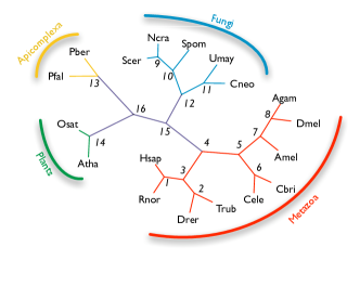
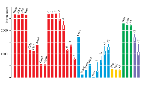
We compiled a data set with 18 eukaryotic species to give a comprehensive picture of spliceosomal evolution among Eukaryotes.

Species	Abbreviation	Assembly	Source
Homo sapiens	Hsap	36.2	R
Rattus norvegicus	Rnor	RGSC 3.4	E
Takifugu rubripes	Trub	FUGU 4.0	E
Danio rerio	Drer	Zv6	E
Drosophila melanogaster	Dmel	BDGP 4.3	R
Anopheles gambiæ	Agam	AgamP3	R
Apis mellifera	Amel	AMEL4.0	R
Cænorhabditis elegans	Cele	WS160	R
Cænorhabditis briggsæ	Cbri	CB25	W
Saccharomyces cerevisiæ	Scer	2.1	R
Neurospora crassa OR74A	Ncer		R
Schizosaccharomyces pombe 972h-	Spom	1.1	R
Ustilago maydis 521	Umay		R
Cryptococcus neoformans v. n. JEC21	Cneo	1.1	R
Oryza sativa ssp. japonica	Osat	RAP 3	R
Arabidopsis thaliana	Atha	6.0	R
Plasmodium falciparum 3D7	Pfal	1.1	R
Plasmodium berghei str. ANKA	Pber		R

Table 4: Data sources and species abbreviations. R: RefSeq release 20, E: Ensemble release 42, W: WormBase release 160.

Data preparation

Genbank flatfiles and protein sequences were downloaded from RefSeq RefSeq2007 and Ensembl Ensembl2007. Exon-intron annotation was extracted from the Genbank flatfiles. The C. briggsæ protein sequences and genome annotation were downloaded from WormBase WormBase2007, and intron annotation was extracted from the GFF annotation file. Table 4 lists the data sources and the species abbreviations. We used the 684 ortholog sets, each corresponding to a cluster of orthologous groups, or KOG COG.new, from the study of Rogozin.data as “seeds” for compiling a set of putative orthologs for our species. For each seed (consisting of homologous protein sequences for eight species), we performed a position-specific iterated BLAST search BLAST. In case of Plasmodium species, we used three iterations against a database of all protozoan peptide sequences in RefSeq. We used an E-value cutoff of $10^{-9}$ for retaining candidates. Each candidate hit was then used as a query in a reversed position-specific BLAST (rpsblast) search CDD2007 against the KOG database. Candidates were retained after this point if they had the highest scoring hit (by rpsblast) against the same KOG as the KOG of the seed data, and they scored within 80% of the best such hit for the species.

Figure 4: Phylogeny for the 18 species and estimated intron counts at ancestors. Ancestral nodes are identified by the numbers 1–16. Error bars denote 95% confidence intervals computed from 1000 simulated data sets. We rooted the tree at node 16 (Bikonts) for computational purposes.

From the resulting set of paralogs, we selected a putative ortholog set in the following manner. For each KOG, we selected all possible triples of human-Arabidopsis-Saccharomyces paralogs and kept the triple that had the highest score in alignments built by MUSCLE MUSCLE. Alignment score was computed using the VTML240 matrix VTML. Additional putative orthologs were added for one species at a time, by aligning each paralog individually to the current profile, and keeping the one that gave the largest alignment score. At this iterative addition, scoring was done with the VTML240 matrix, by summing the five highest pairwise scores between a candidate and already included sequences.

The resulting sets were then realigned using MUSCLE, and then realigned again using our intron-aware alignment with a gap penalty of 300, gap-extend penalty of 11, VTML240 amino acid scoring, intron-match scores of 300 and intron-mismatch penalties of 20. (These latter were established using different intron-match and -mismatch scores, and selecting the ones that gave the fewest number of intron sites while decreasing the score of the implied protein alignment by less than 0.1%.)

Conserved portions were extracted using our segmentation program with a complexity penalty of $\alpha=400$ (larger values gave identical segmentation results, and lower values resulted in too many scattered blocks). We penalized indels with an infinitely large value to exclude gap columns. Phase-0 introns falling on the boundaries of conserved blocks were excluded. Intron presence and absence in the aligned data was then extracted to produce the data for the likelihood programs.

Results

Figure 4 shows the estimated intron densities for ancestral species. It is notable that ancestral nodes such as the bilaterian ancestor (node 4), the ecdysozoan ancestor (node 5), the opisthokont ancestor (node 15), and the bikont ancestor (node 16) all have very high intron densities, surpassing most previous estimates Rogozin.data,csuros.scenarios. The ecdysozoan ancestor has an even higher estimated intron density (80% of human density) than the otherwise quite generous estimates (about 70%) of RoyGilbert.earlygenes, which is mostly due to the inclusion of the relatively intron-rich honeybee genes honeybee. Intron density in the bilaterian ancestor is estimated to be almost as high as in humans (94%), agreeing with estimates of RoyGilbert.earlygenes. Sequences of a handful of intron-rich genes from the marine annelid Platynereis dumerilii have already indicated that the bilaterian ancestor’s genome was at least two-thirds as intron-rich as the vertebrate genomes even by conservative estimates introns.dumerilii,Roy.dumerilii.

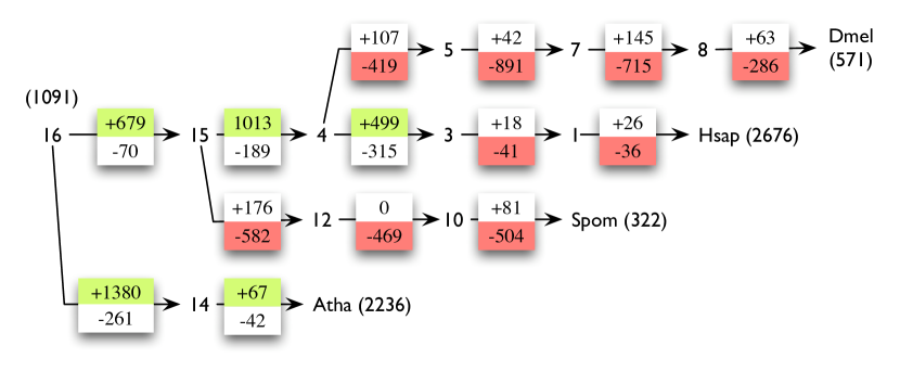
Introns are for the most part lost on the branches. Figure 5 shows the estimated changes in a few lineages. Intron evolution has been much slower in the vertebrate lineage than in most other lineages: in more than 380 million years since the divergence with fishes, only about 3% of our introns got lost. Fungi, for example, massively trimmed their introns in many lineages. A notable exception is C. neoformans, which seems to have gained introns, but that assessment may change if another basidiomycete genome becomes available besides the relatively intron-poor U. maydis.

Figure 5: Intron gains and losses in a few evolutionary paths. Estimated and actual intron counts are in parentheses.

6 Conclusion

We presented a novel alignment technique for establishing intron orthology, and a likelihood framework in which intron evolutionary events can be quantified. We described a compression method for the evaluation of the likelihood function, which has been extremely valuable in practice. We also showed that the compression leads to sublinear running times for likelihood evaluation.

We illustrated our methods for analyzing intron evolution with a large and diverse set of eukaryotic organisms. The data set is more comprehensive than any used in other studies published to this day. The data indicate that ancestral eukaryotic genomes were more intron-rich than previous studies suggested.

Many circumstances influence intron loss Jeffares.gainloss,RoyGilbert.review, and realistic likelihood models need to introduce rate variation Carmel.EM. Usual rate variation models Felsenstein entail multiple evaluations of the likelihood function, and, thus, underline the importance of computational efficiency. We believe that the proposed methods will help to produce and analyze large data sets even within complicated likelihood models.

References

- [\citeauthoryearAdachi and HasegawaAdachi and Hasegawa1995] Adachi, J. and M. Hasegawa (1995). MOLPHY version 2.3: programs for molecular phylogenetics based on maximum likelihood. Volume 28 of Computer Science Monographs, pp. 1–150. Tokyo, Japan: Institute of Statistical Mathematics.
- [\citeauthoryearAldousAldous2001] Aldous, D. (2001). Stochastic models and descriptive statistics for phylogenetic trees, from Yule to today. Statistical Science 16, 23–34.
- [\citeauthoryearAltschul, Madden, Schäffer, Zhang, Zhang, Miller, and LipmanAltschul et al.1997] Altschul, S. F., T. L. Madden, A. A. Schäffer, J. Zhang, Z. Zhang, W. Miller, and D. J. Lipman (1997). Gapped BLAST and PSI-BLAST: a new generation of protein database search programs. Nucleic Acids Research 25(17), 3389–3402.
- [\citeauthoryearBieri et al.Bieri et al.2007] Bieri, T. et al. (2007). WormBase: new content and better access. Nucleic Acids Research 35(suppl_1), D506–510.
- [\citeauthoryearBlum and FrançoisBlum and François2005] Blum, M. G. B. and O. François (2005). On statistical tests of phylogenetic tree imbalance: The Sackin and other indices revisited. Mathematical Biosciences 195, 141–153.
- [\citeauthoryearCarmel, Rogozin, Wolf, and KooninCarmel et al.2005] Carmel, L., I. B. Rogozin, Y. I. Wolf, and E. V. Koonin (2005). An expectation-maximization algorithm for analysis of evolution of exon-intron structure of eukaryotic genes. See \citeNRCG2005, pp. 35–46.
- [\citeauthoryearCollins and PennyCollins and Penny2005] Collins, L. and D. Penny (2005). Complex spliceosomal organization ancestral to extant eukaryotes. Molecular Biology and Evolution 22(4), 1053–1066.
- [\citeauthoryearCoulombe-Huntington and MajewskiCoulombe-Huntington and Majewski2007] Coulombe-Huntington, J. and J. Majewski (2007). Characterization of intron loss events in mammals. Genome Research 17(1), 23–32.
- [\citeauthoryearCsűrösCsűrös2004] Csűrös, M. (2004). Maximum-scoring segment sets. IEEE/ACM Transactions on Computational Biology and Bioinformatics 1(4), 139–150.
- [\citeauthoryearCsűrösCsűrös2005] Csűrös, M. (2005). Likely scenarios of intron evolution. See \citeNRCG2005, pp. 47–60. DOI:10.1007/11554714_5.
- [\citeauthoryearDevroyeDevroye1991] Devroye, L. (1991). Limit laws for local counters in random binary search trees. Random Structures and Algorithms 2(1), 303–315.
- [\citeauthoryearDurbin, Eddy, Krogh, and MitchisonDurbin et al.1998] Durbin, R., S. R. Eddy, A. Krogh, and G. Mitchison (1998). Biological Sequence Analysis: Probabilistic Models of Proteins and Nucleic Acids. UK: Cambridge University Press.
- [\citeauthoryearEdgarEdgar2004] Edgar, R. C. (2004). MUSCLE: multiple sequence alignment with high accuracy and high throughput. Nucleic Acids Research 32(5), 1792–1797.
- [\citeauthoryearFelsensteinFelsenstein1981] Felsenstein, J. (1981). Evolutionary trees from DNA sequences: A maximum likelihood approach. Journal of Molecular Evolution 17, 368–376.
- [\citeauthoryearFelsensteinFelsenstein1992] Felsenstein, J. (1992). Phylogenies from restriction sites, a maximum likelihood approach. Evolution 46, 159–173.
- [\citeauthoryearFelsensteinFelsenstein2004] Felsenstein, J. (2004). Inferring Pylogenies. Sunderland, Mass.: Sinauer Associates.
- [\citeauthoryearFriedman, Ninio, Pupko, Pe’er, and PupkoFriedman et al.2002] Friedman, N., M. Ninio, T. Pupko, I. Pe’er, and T. Pupko (2002). A structural EM algorithm for phylogenetic inference. Journal of Computational Biology 9(2), 331–353.
- [\citeauthoryearGuindon and GascuelGuindon and Gascuel2003] Guindon, S. and O. Gascuel (2003). A simple, fast, and aaccurate accurate algorithm to estimate large phylogenies by maximum likelihood. Systematic Biology 52(5), 696–704.
- [\citeauthoryearHardingHarding1971] Harding, E. (1971). The probabilities of rooted tree-shapes generated by random bifurcation. Advances in Applied Probability 3, 44–77.
- [\citeauthoryearHeardHeard1992] Heard, S. B. (1992). Patterns in tree balance among cladistic, phenetic, and randomly generated phylogenetic trees. Evolution 46(6), 1818–1826.
- [\citeauthoryearHubbard et al.Hubbard et al.2007] Hubbard, T. J. P. et al. (2007). Ensembl 2007. Nucleic Acids Research 35(suppl_1), D610–617.
- [\citeauthoryearIHBSCIHBSC2006] IHBSC (2006). Insights into social insects from the genome of the honey bee Apis mellifera. Nature 443, 931–949.
- [\citeauthoryearJeffares, Mourier, and PennyJeffares et al.2006] Jeffares, D. C., T. Mourier, and D. Penny (2006). The biology of intron gain and loss. Trends in Genetics 22(1), 16–22.
- [\citeauthoryearKececioglu and ZhangKececioglu and Zhang1998] Kececioglu, J. and W. Zhang (1998). Aligning alignments. In M. Farach-Colton (Ed.), Proc. CPM, Volume 1448 of LNCS, pp. 189–208. Springer.
- [\citeauthoryearMa, Wang, and ZhangMa et al.2003] Ma, B., Z. Wang, and K. Zhang (2003). Alignment between two multiple alignments. In R. A. Baeza-Yates, E. Chávez, and M. Crochemore (Eds.), Proc. Combinatorial Pattern Matching (CPM), Volume 2676 of LNCS, pp. 254–265. Springer.
- [\citeauthoryearMarchler-Bauer et al.Marchler-Bauer et al.2007] Marchler-Bauer, A. et al. (2007). CDD: a conserved domain database for interactive domain family analysis. Nucleic Acids Research 35(suppl_1), D237–240.
- [\citeauthoryearMcDiarmidMcDiarmid1989] McDiarmid, C. (1989). On the method of bounded differences. In J. Siemons (Ed.), Surveys in Combinatorics, pp. 148–184. Cambridge University Press.
- [\citeauthoryearMcKenzie and SteelMcKenzie and Steel2000] McKenzie, A. and M. Steel (2000). Distributions of cherries for two models of trees. Mathematical Biosciences 164, 81–92.
- [\citeauthoryearMcLysaght and HusonMcLysaght and Huson2005] McLysaght, A. and D. Huson (Eds.) (2005). Proc. RECOMB Satellite Workshop on Comparative Genomics, Volume 3678 of LNCS. Springer-Verlag.
- [\citeauthoryearMüller, Spang, and VingronMüller et al.2002] Müller, T., R. Spang, and M. Vingron (2002). Estimating amino acid substitution models: a comparison of Dayhoff’s estimator, the resolvent approach and a maximum likelihood method. Molecular Biology and Evolution 19(1), 8–13.
- [\citeauthoryearNguyen, Yoshihama, and KenmochiNguyen et al.2005] Nguyen, H. D., M. Yoshihama, and N. Kenmochi (2005). New maximum likelihood estimators for eukaryotic intron evolution. PLoS Computational Biology 1(7), e79.
- [\citeauthoryearNielsen, Friendman, Birren, Burge, and GalaganNielsen et al.2004] Nielsen, C. B., B. Friendman, B. Birren, C. B. Burge, and J. E. Galagan (2004). Patterns of intron gain and loss in fungi. PLoS Biology 2(12), e422.
- [\citeauthoryearNixon, Wang, Morrison, McArthur, Sogin, Loftus, and SamuelsonNixon et al.2002] Nixon, J. E. J., A. Wang, H. G. Morrison, A. G. McArthur, M. L. Sogin, B. J. Loftus, and J. Samuelson (2002). A spliceosomal intron in Giardia lamblia. Proceedings of the National Academy of Sciences of the USA 99(6), 3701–3705.
- [\citeauthoryearPress, Teukolsky, Vetterling, and FlanneryPress et al.1997] Press, W. H., S. A. Teukolsky, W. V. Vetterling, and B. P. Flannery (1997). Numerical Recipes in C: The Art of Scientific Computing (Second ed.). Cambridge UniversIty Press.
- [\citeauthoryearPruitt, Tatusova, and MaglottPruitt et al.2007] Pruitt, K. D., T. Tatusova, and D. R. Maglott (2007). NCBI reference sequences (RefSeq): a curated non-redundant sequence database of genomes, transcripts and proteins. Nucleic Acids Research 35(suppl_1), D61–65.
- [\citeauthoryearRaible, Tessmar-Raible, Osoegawa, Wincker, Jubin, Balavoine, Ferrier, Benes, de Jong, Weissenbach, Bork, and ArendtRaible et al.2005] Raible, F., K. Tessmar-Raible, K. Osoegawa, P. Wincker, C. Jubin, G. Balavoine, D. Ferrier, V. Benes, P. de Jong, J. Weissenbach, P. Bork, and D. Arendt (2005). Vertebrate-type intron-rich genes in the marine annelid Platynereis dumerilii. Science 310, 1325–1326.
- [\citeauthoryearRogozin, Sverdlov, Babenko, and KooninRogozin et al.2005] Rogozin, I. B., A. V. Sverdlov, V. N. Babenko, and E. V. Koonin (2005). Analysis of evolution of exon-intron structure of eukaryotic genes. Briefings in Bioinformatics 6(2), 118–134.
- [\citeauthoryearRogozin, Wolf, Sorokin, Mirkin, and KooninRogozin et al.2003] Rogozin, I. B., Y. I. Wolf, A. V. Sorokin, B. G. Mirkin, and E. V. Koonin (2003). Remarkable interkingdom conservation of intron positions and massive, lineage-specific intron loss and gain in eukaryotic evolution. Current Biology 13, 1512–1517.
- [\citeauthoryearRosenbergRosenberg2006] Rosenberg, N. A. (2006). The mean and variance of -pronged nodes and -caterpillars in Yule-generated genealogies. Annals of Combinatorics 10, 129–146.
- [\citeauthoryearRossRoss1996] Ross, S. M. (1996). Stochastic Processes (Second ed.). Wiley & Sons.
- [\citeauthoryearRoyRoy2006] Roy, S. W. (2006). Intron-rich ancestors. Trends in Genetics 22(9), 468–471.
- [\citeauthoryearRoy and GilbertRoy and Gilbert2005] Roy, S. W. and W. Gilbert (2005). Complex early genes. Proceedings of the National Academy of Sciences of the USA 102(6), 1986–1991.
- [\citeauthoryearRoy and GilbertRoy and Gilbert2006] Roy, S. W. and W. Gilbert (2006). The evolution of spliceosomal introns: patterns, puzzles and progress. Nature Reviews Genetics 7, 211–221.
- [\citeauthoryearRoy and PennyRoy and Penny2006] Roy, S. W. and D. Penny (2006). Large-scale intron conservation and order-of-magnitude variation in intron loss/gain rates in apicomplexan evolution. Genome Research 16(10), 1270–1275.
- [\citeauthoryearRoy and PennyRoy and Penny2007] Roy, S. W. and D. Penny (2007). Patterns of intron loss and gain in plants: Intron loss-dominated evolution and genome-wide comparison of O. sativa and A. thaliana. Molecular Biology and Evolution 24(1), 171–181.
- [\citeauthoryearStamatakis, Ludwig, Meier, and WolfStamatakis et al.2002] Stamatakis, A. P., T. Ludwig, H. Meier, and M. J. Wolf (2002). AxML: A fast program for sequential and parallel phylogenetic tree calculations based on the maximum likelihood method. In Proc. IEEE Computer Society Bioinformatics Conference (CSB), pp. 21–28.
- [\citeauthoryearSteelSteel1994] Steel, M. A. (1994). Recovering a tree from the leaf colourations it generates under a Markov model. Applied Mathematics Letters 7, 19–24.
- [\citeauthoryearSverdlov, Csűrös, Rogozin, and KooninSverdlov et al.2007] Sverdlov, A. V., M. Csűrös, I. B. Rogozin, and E. V. Koonin (2007). A glimpse of a putative pre-intron phase of eukaryotic evolution. Trends in Genetics. In press. DOI: /10.1016/j.tig.2007.01.001.
- [\citeauthoryearSverdlov, Rogozin, Babenko, and KooninSverdlov et al.2005] Sverdlov, A. V., I. B. Rogozin, V. N. Babenko, and E. V. Koonin (2005). Conservation versus parallel gains in intron evolution. Nucleic Acids Research 33(6), 1741–1748.
- [\citeauthoryearTatusov et al.Tatusov et al.2003] Tatusov, R. L. et al. (2003). The COG database: an updated version includes eukaryotes. BMC Bioinformatics 4, 441.
- [\citeauthoryearVaňáčová, Yan, Carlton, and JohnsonVaňáčová et al.2005] Vaňáčová, Š., W. Yan, J. M. Carlton, and P. J. Johnson (2005). Spliceosomal introns in the deep-branching eukaryote Trichomonas vaginalis. Proceedings of the National Academy of Sciences of the USA 102(12), 4430–4435.
- [\citeauthoryearZhang, Berman, Wiehe, and MillerZhang et al.1999] Zhang, Z., P. Berman, T. Wiehe, and W. Miller (1999). Post-processing long pairwise alignments. Bioinformatics 15(12), 1012–1019.