Attribute Exploration of Discrete Temporal Transitions

Abstract

Discrete temporal transitions occur in a variety of domains, but this work is mainly motivated by applications in molecular biology: explaining and analyzing observed transcriptome and proteome time series by literature and database knowledge. The starting point of a formal concept analysis model is presented. The objects of a formal context are states of the interesting entities, and the attributes are the variable properties defining the current state (e.g. observed presence or absence of proteins). Temporal transitions assign a relation to the objects, defined by deterministic or non-deterministic transition rules between sets of pre- and postconditions. This relation can be generalized to its transitive closure, i.e. states are related if one results from the other by a transition sequence of arbitrary length. The focus of the work is the adaptation of the attribute exploration algorithm to such a relational context, so that questions concerning temporal dependencies can be asked during the exploration process and be answered from the computed stem base. Results are given for the abstract example of a game and a small gene regulatory network relevant to a biomedical question.

1 Introduction

Discrete temporal transitions occur in a variety of domains: control of engineering processes or roboters, flow of computer programs, a piece of music, games, etc. We are mainly interested in biological applications, but we develop a formal structure as widely usable as possible.

The practical aim is to explain experimental time series in molecular biology or to hypothesize about temporal developments, especially in the context of gene expression regulation. Its first step is transcription, i.e. the synthesis of mRNA from a DNA sequence coding for a gene. Concentrations of mRNA for all genes of a cell culture (transcriptome analysis) can be measured by the rather new technique of microarrays (RNA binds to matching fragments of DNA or RNA fixed on a chip). The second step of gene expression is the translation of the mRNA into multiple identical proteins by ribosomes. Since the mRNA concentrations are only weakly correlated to the respective protein concentrations, it is recommended to also measure the latter, i.e. to perform proteome analysis. However, it is unfavourable that weakly expressed proteins remain undetectable. By complex - activating or inactivating - interactions of proteins within or between cells (signaling pathways), a special class of proteins can be activated and - if necessary - transported to the cell nucleus. Those transcription factors again regulate the expression of a sometimes large set of genes.

At a more global level, such cycles are described as gene regulatory networks (Figure 1). One abstracts from biochemical activation processes of proteins; only the mRNA or protein level is considered as the main influencing factor. The indirect interactions between genes are positive (upregulation of expression) or negative (downregulation). Regulatory networks may be constructed based on knowledge available by manual or automatic (text mining) literature search and in biological databases.

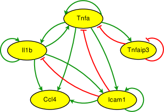
Figure 1: Gene regulatory network. $\rightarrow$ upregulation, $\dashv$ downregulation. The information was obtained from the text mining software PathwayStudio [www.ariadnegenomics.com] and the manually curated protein interaction database Transpath [www.biobase.de].

The network determines the possible transitions between properties of gene products (mRNA or protein levels); as a first approximation they can be either present or absent. In the following we translate similar situations into the language of formal concept analysis (FCA), so that attribute exploration [3, 85ff.] can be applied. During this interactive algorithm, an expert is asked about the general validity of basic implications $A\rightarrow B$ between the attributes of a given formal context $(G,M,I)$. An implication has the meaning: ”If an object $g\in G$ has all attributes $a\in A\subseteq M$, then it has also all attributes $b\in B\subseteq M$.” If the expert denies, he must provide a counterexample, i.e. a new object of the context. If he accepts, the implication is added to the stem base (Duquenne-Guigues base) of the context. At the end, all implications valid in the possibly enlarged context can be derived from the minimal set of rules contained in the stem base. Those are identical to the implications valid in the explored domain according to the knowledge available to the expert.

The present work is based on a FCA modeling of temporal transitions in [4]. The biological application is influenced by computation tree logic [1], Boolean networks [5] and qualitative reasoning [6]. Temporal concept analysis as developed by K.E. Wolff [7] is more directed toward a description of temporal concepts than toward temporal logic. In future work, we shall investigate existing analogies and take advantage of them.

2 Methods - Basic Definitions

We start with two sets:

• The universe $E$. The elements of $E$ will be called entities. They represent the objects of the world which we are interested in.

• The set $F$ (fluents) denotes changing properties of the entities.

A state of the universe is characterized by a unique value in $F$ taken by every $e\in E$; states with the same attribute values are identified. Therefore a state can be defined as a map $\varphi:E\rightarrow F$. If the state is not completely known, $\varphi$ is a partial map. To explore static features of states, the following formal context is defined as a special case of a many-valued context [3, 36ff.]. An example of an attribute exploration of a state context (defined as a single-valued context and with a slightly more general notion of a state) is given in [4, 4.1.].

Definition 1

Given two sets $E$ (entities) and $F$ (fluents), a state context is a many-valued context $(G,E,F,J)$ with $G\subseteq\{\varphi:E\rightarrow F\}$; its relation $J$ is given as $(\varphi,e,f)\in J\Leftrightarrow\varphi(e)=f$, for all $\varphi\in G,e\in E$ and $f\in F$.

The class of these contexts is well defined; since $\varphi$ is a map, the property of a many-valued context is fulfilled: $(\varphi,e,f_{1})\in J\wedge(\varphi,e,f_{2})\in J\Rightarrow f_{1}=f_{2}.$ If a many-valued attribute is regarded as a partial map from $G$ into $F$, one can also write $e(\varphi)=f$.

For each attribute $e\in E$, a scale can be defined, i.e. a one-valued context $S_{e}:=(G_{e},M_{e},J_{e})$ with $e(G)\subseteq G_{e}$. Thus by plain scaling we derive from $(G,E,F,J)$ the context $(G,M,I)$ with

$$M:=\bigcup_{e\in E}e\times M_{e},\text{ and}$$ (1)

$$\varphi I(e,m_{e}):\Leftrightarrow e(\varphi)=f\text{ and }fI_{e}m_{e}.\$$ (2)

If $\forall e\in E:M_{e}\subseteq F$, we get $M\subseteq E\times F$. This is the case e.g. for nominal, ordinal and dichotomic scales. For nominal and dichotomic scales, the relation $I$ simply is defined by $\varphi\,I\,(e,f):\Leftrightarrow\varphi(e)=f$; the following text is based on this relation.

Now we need a supplementary structure: a relation $R\subseteq G\times G$ indicates temporal transitions between the states. A deterministic relation may be given by a family of elementary transition rules: preconditions / postconditions $(V_{k},N_{k})_{k\in K}$, $V_{k},N_{k}\subseteq M$, so that

$$(\varphi_{0},\varphi_{1})\in R\Leftrightarrow\forall k\in K:V_{k}\subseteq\varphi_{0}^{\prime}\Rightarrow N_{k}\subseteq\varphi_{1}^{\prime}.$$ (3)

In the non-deterministic case (e.g. for a game), different postconditions are possible. There is a class of families $\{(V_{k},N_{k}^{l})_{k\in K}|\>l\in L_{k}\text{ for all }k\in K\}$, and

$$\forall k\in K:V_{k}\subseteq\varphi_{0}^{\prime}\Rightarrow\exists l\in L_{k}:N_{k}^{l}\subseteq\varphi_{1}^{\prime}$$ (4)

The relational context $((G,R),M,I)$ can be represented by a binary power context family. Here we prefer the equivalent context, analoguous to [4, Definition 4]:

Definition 2

Given a state context $(G,E,F,J)$ and a relation $R\subseteq G\times G$, a transition context $\mathcal{K}$ is the context $(R,M\times\{0,1\},\tilde{I})$, $M\subset E\times F$, with the property

$$\forall i\in\{0,1\}\!:\>(\varphi_{0},\varphi_{1})\tilde{I}(e,f,i)\Leftrightarrow\varphi_{i}(e)=f.$$ (5)

It appears promising to consider the transitive closure $t(R)=\bigcup_{n\in\mathbb{N}}R^{n}$, i.e. $\varphi_{0}\,t(R)\,\varphi_{1}$ for any elements $\varphi_{0}$ and $\varphi_{1}$ of $G$, provided there exist $\alpha_{0},\alpha_{1},...,\alpha_{n}\in G$ with $\alpha_{0}=\varphi_{0},\alpha_{n}=\varphi_{1}$, and $\alpha_{r}R\alpha_{r+1}$ for all $0\leq r<n$. That means, the state $\varphi_{1}$ emerges from $\varphi_{0}$ by some transition sequence of arbitrary length. So we get a new transitive context

$$\mathcal{K}_{t}:=((G,t(R)),M,I)\,\hat{=}\,(t(R),M\times\{0,1\},\tilde{\tilde{I}}).$$ (6)

The relation $\tilde{\tilde{I}}$ is defined like ${\tilde{I}}$ in (5).

Regarding this context, queries like the following are possible, for $A,B,C\subseteq M,$ $m\in M$ (compare [1, 37], [6, 2020f.]). In a non-deterministic setting, the implications (7) and (9) refer to all possible transition paths starting from a state $\varphi_{0}$ with all attributes $b\in B$. According to computation tree logic [1, 33], one could also ask if a path exists with the respective property. (8) expresses that in the future development of $\varphi_{0}$, there will be a state with attribute $m$ for at least one path.

$$B\rightarrow\text{never}(m)\> \Leftrightarrow\>(B\times\{0\})^{\prime}\cap(m,1)^{\prime}=\emptyset$$ (7)

$$B\rightarrow\text{eventually}(m)\> \Leftrightarrow\>(B\times\{0\})^{\prime}\cap(m,1)^{\prime}\neq\emptyset$$ (8)

$$B\rightarrow\text{always}(m)\> \Leftrightarrow\>(B\times\{0\})^{\prime}\subseteq(m,1)^{\prime}$$ (9)

$$\exists\text{ stable state or oscillation}\> \Leftrightarrow\>\exists B\subset M:(B\times\{0\})^{\prime}\cap(B\times\{1\})^{\prime}\neq\emptyset$$ (10)

Given a (partial) initial state $$A$$, can the system (11)

reach the state $$C B$$ while passing by another state ?

$$\Leftrightarrow (A\times\{0\})^{\prime}\cap(B\times\{1\})^{\prime}\neq\emptyset\>\wedge\,(B\times\{0\})^{\prime}\cap(C\times\{1\})^{\prime}\neq\emptyset$$

Those queries can also be checked for contexts modified by omitting some transition rules. So one can investigate, if certain interactions are necessary for specific state transitions.

The attribute exploration process has to be adapted, so that similar questions can be asked as implications during the exploration and be answered from the computed stem base. The following equivalences are straightforward:

$$B\rightarrow\text{never}(m)\> \Leftrightarrow\>B\times\{0\}\cup(m,1)\rightarrow\bot$$ (12)

$$B\rightarrow\text{always}(m)\> \Leftrightarrow\>B\times\{0\}\rightarrow(m,1)$$ (13)

A counterexample has to be introduced into the context, if the temporal property in question is in contradiction to the data or to the desired behaviour of the system which is to be designed.

3 Results - Two Examples

In this section a state transition $(\varphi_{0},\varphi_{1})$ is written as $(\varphi^{in},\varphi^{out})$, and attributes are noted as $m^{in}$ or $m^{out}$ instead of $(m,0)$ or $(m,1)$.

3.1 3-pawns-chess

In order to get a widely applicable view on discrete state transitions, the abstract case of a simple game is introduced. It resembles chess with only three pawns. The game is won when a pawn reaches the opposite side or when the opponent is blocked from further moves. Below are listed all states reachable from a state $\varphi^{in}_{0}$ (0. - two moves after the beginning), and the bar marks the next player. The following transitions are possible:

$(\varphi^{in}_{0},\varphi^{out}_{1})$, $(\varphi^{in}_{0},\varphi^{out}_{2})$, $(\varphi^{in}_{0},\varphi^{out}_{3})$;

$(\varphi^{in}_{1},\varphi^{out}_{4})$;

$(\varphi^{in}_{2},\varphi^{out}_{5})$, $(\varphi^{in}_{2},\varphi^{out}_{6})$ (similar transitions are not listed);

$(\varphi^{in}_{3},\varphi^{out}_{7})$.

In states 4, 5 and 7, black wins, in 6 white.

1. 
   

1. 
   

1. 
   

Our basic sets are $E=(\{a,b,c\}\times\{1,2,3\})\>\cup$ {move, win}, $F$ = {white, black}. $G$, the set of all possible states of the game, is a proper subset of $\{\varphi:E\rightarrow F\}$. Some examples of the attributes are a1.white, move.white or win.black. The state context $(G,E,F,J)$ is not complete, because in every situation there are at least 3 empty fields, and not every state is a win-situation; there exist $e\in E$, so that the domain $D$ of the corresponding map $e:D\subseteq G\rightarrow F$ is not equal to $G$.

Starting from the context with the transitive relation for the states 0. to 7., the stem base was computed. Among others, the following of the 61 implications are of some interest ($\top$ denotes the empty set of preconditions, $\bot:=M$ provided $M^{\prime}=\emptyset$):

• $\top\rightarrow$ a3.blackⁱⁿ, c3.blackⁱⁿ, a3.black^out: a3 is always occupied by black, c3 always but in the last step.

• b2.black^out $\rightarrow\bot$: b2.black^out characterizes an impossible game situation.

• a2.white^out, move.white^out $\rightarrow$ c2.black^out, win.black^out: For white, this implication could be a warning not to move to a2.

• a2.black^out, move.white^out $\rightarrow$ win.white^out: This confirms the tactic importance of a2.

• c3.black^out, move.white^out $\rightarrow$ a1.black^out, win.black^out: another winning condition.

3.2 Gene regulatory networks

We want to provide a temporal semantics for gene regulatory events, e.g. ”gene1 upregulates the expression of gene2”. So the entities $E$ are the interesting genes, and the fluents $F$ = {abs, pres} = {-,+} are mRNA or protein levels.

In this section, the biological application of the present approach is explained by the example of the 5 gene network of Figure 1. We confine ourselves to a single measured time series of mRNA concentrations. It is part of ongoing biomedical research directed toward the understanding of complex molecular interactions relevant for the pathogenensis and therapy of rheumatoid arthritis (RA). This disease putatively has autoimmune causes, and it is recognized that proteins like Tnf$\alpha$ and Il1$\beta$ - responsible for intercellular communication - have a major stimulating influence on the inflammatory process [2]. Therefore fibroblasts (particular cells of the joint) from RA patients were stimulated with Tnf$\alpha$, and their expression was monitored by Affymetrix U133 Plus 2.0 microarrays before and 1, 2, 4 and 12 hours after stimulation. mRNA levels were grouped into the two classes absent and present. One resulting time course is shown in Table 1 as a transition context $\mathcal{K}^{obs}$ according to Definition 2.

Now a corresponding knowledge based context will be developed. State transitions are computed according to (3): all rules of one family are applied with preconditions matching the attributes of the input state $\varphi^{in}$. The type of rules valid for particular genes is determined by the regulatory network (Figure 1). Table 2 lists some basic rule types; they are sufficient to compute the 2-gene transition context of Table 3.

Table 1: Observed transition context $\mathcal{K}^{obs}$.

Transition	Tnf$\alpha^{in}$	Tnfaip3in	Icam1in	Ccl4in	Il1$\beta^{in}$	Tnf$\alpha^{out}$	Tnfaip3out	Icam1out	Ccl4out	Il1$\beta^{out}$
$(\varphi_{0}^{in},\varphi_{1}^{out})$	+	-	-	-	-	+	+	+	+	-
$(\varphi_{1}^{in},\varphi_{2}^{out})$	+	+	+	+	-	+	+	+	+	+
$(\varphi_{2}^{in},\varphi_{3}^{out})$	+	+	+	+	+	+	+	+	+	-
$(\varphi_{3}^{in},\varphi_{4}^{out})$	+	+	+	+	-	-	+	+	-	+

Table 2: Transition rules (simplified notation).

Nr.	Meaning	Rule
1	Upregulation	gene1.pres $\rightarrow$ gene2.pres
2a	Downregulation	gene1.pres, gene2.pres $\rightarrow$ gene3.abs
2b	Failed downregulation	gene1.pres, gene2.pres $\rightarrow$ gene3.pres
2c	No downregulation	gene1.pres, gene2.abs $\rightarrow$ gene3.pres
3	Degradation	gene.pres $\rightarrow$ gene.abs
4	No effect	gene.abs $\rightarrow$ gene.abs

Rules 3 and 4 are default rules; they are only applied to genes not occurring at the right side of another rule. Since the model abstracts from exact thresholds and time delays (which are rarely known), there are the alternative downregulation rules 2a and 2b. After one time step, upregulation or downregulation can prevail. (By the same reason, one could add to rule 3 the alternative gene.present $\rightarrow$ gene.present.) The model is non-deterministic, the context $\mathcal{K}$ of Table 3 shows the possible state transitions, starting from the initial state $\varphi^{in}_{0}$ of the individual time series $\mathcal{K}^{obs}$. It could also be relevant to investigate contexts containing the initial states of different observed cellular conditions, different patients or with all possible input states.

Table 3: Knowledge based transition context $\mathcal{K}$ for 2 genes. Example rules for $(\varphi_{1}^{in},\varphi_{2}^{out})$: Tnf$\alpha$.pres, Tnfaip3.pres $\rightarrow$ Tnf$\alpha$.abs (2a); Tnf$\alpha$.pres, Tnfaip3.pres $\rightarrow$ Tnfaip3.pres (2b).

Transition	Tnf$\alpha^{in}$	Tnfaip3in	Tnf$\alpha^{out}$	Tnfaip3out	Applied rules
$(\varphi_{0}^{in},\varphi_{1}^{out})$	+	-	+	+	2c
$(\varphi_{1}^{in},\varphi_{0}^{out})$	+	+	+	-	2b,2a
$(\varphi_{1}^{in},\varphi_{1}^{out})$	+	+	+	+	2b
$(\varphi_{1}^{in},\varphi_{2}^{out})$	+	+	-	+	2a,2b
$(\varphi_{1}^{in},\varphi_{3}^{out})$	+	+	-	-	2a
$(\varphi_{2}^{in},\varphi_{3}^{out})$	-	+	-	-	4,3
$(\varphi_{3}^{in},\varphi_{3}^{out})$	-	-	-	-	4

Implications of this context $\mathcal{K}$ simply reflect the rules applied in order to compute a state transition. Deterministic transition rules even may be included in the stem base of the context, or they follow from it. (Of course, the stem base contains also implications in the inverse direction - from output to input attributes - or mixed implications like gene1.pres^out, gene2.abs${}^{in}\rightarrow$ gene3.presⁱⁿ.)

The transitive context $\mathcal{K}_{t}$ is derived from $\mathcal{K}$ by adding all supplementary objects $(\varphi^{in},\varphi^{out})\in t(R)$. An interactive attribute exploration of $\mathcal{K}$ may be more intuitive than an exploration of $\mathcal{K}_{t}$; the expert can compare the implications in question to the measured one step transitions of $\mathcal{K}^{obs}$ and eventually check them against supplementary knowledge. However, a time step of a knowledge based transition is not identical to a measurement interval; the problem is aggravated, if the intervals are different as in the present case. Therefore it seems more appropriate to explore the transitive context $\mathcal{K}_{t}$ immediately. Its implications denote dependencies between attributes of states related by transitions of arbitrary duration. The following procedure was applied:

1. Transform a time series of gene expression measurements to an observed context $\mathcal{K}^{obs}$.

2. For a set of interesting genes, extract transition rules from biological literature and databases.

3. Construct the transition context $\mathcal{K}$, starting from $\varphi^{in}_{0}$ of $\mathcal{K}^{obs}$.

4. Derive the respective transitive contexts $\mathcal{K}_{t}$ and $\mathcal{K}^{obs}_{t}$.

5. Perform attribute exploration of $\mathcal{K}_{t}$. Decide about an implication $A\rightarrow B$ by checking its validity in $\mathcal{K}^{obs}_{t}$ and/or by searching for supplementary knowledge. Possibly provide a counterexample from $\mathcal{K}^{obs}_{t}$.

6. Answer queries from the modified context $\mathcal{K}_{t}$ and from its stem base.

For all 5 genes Tnf$\alpha$, Tnfaip3, Icam1, Ccl4 and Il1$\beta$, a more complex set of transition rules had to be defined, which we shall not discuss here.

In step 5, automatic decision criteria could be tresholds of support $q=|(A\cup B)^{\prime}|$ and confidence $p=\frac{|(A\cup B)^{\prime}|}{|A^{\prime}|}$ for an implication in $\mathcal{K}^{obs}_{t}$. A weak criterion is to reject only implications with support 0 (but if no object in $\mathcal{K}^{obs}_{t}$ has all attributes from A, the implication is not violated). In the present example a strong criterion was applied: implications of $\mathcal{K}_{t}$ had to be valid also in the observed context. This is equivalent to an exploration of the union of the two contexts. Its results, where all common implications were accepted by the expert, are presented in Table 4. It has to be considered that the combined context generally only represents a transitive relation on the states for its subcontexts $\mathcal{K}_{t}$ and $\mathcal{K}_{t}^{obs}$. The main purpose of the proposed exploration is to make a falsification of the $\mathcal{K}_{t}$ implications possible.

The subsequent implications are noteworthy and biologically meaningful: 1. is equivalent to always(Icam1.pres^out). The same assertion for Ccl4 was falsified by the measurement; instead there are the new implications 2. to 5. and 15. to 17. The static implications 6. and 10. to 13. reflect the very similar regulation of Il1$\beta$, Icam1 and Ccl4 (e.g. by Il1$\beta$ and Tnf$\alpha$) and were also valid in the observed context. Likewise, 14. was supported by a priori and observed transitions. 7. to 9. and 19. to 21. mirror the important role of the upregulating genes Il1$\beta$ and Tnf$\alpha$: if Il1$\beta$, Tnfaip3 or Tnf$\alpha$ are upregulated at an arbitrary time point, either Il1$\beta$ or Tnf$\alpha$ have been present in the past.

Table 4: The stem base of the combined knowledge based and observed transitive contexts. Implications following from the previously entered background implications of the form gene.abs, gene.pres $\rightarrow\bot$ are not shown. The implications are presented in a short form proposed during attribute exploration by the ConImp program (available at http://www.mathematik.tu-darmstadt.de/$\sim$burmeister/ConImp.tar), with basis of premise and/or reduced conclusion.

Nr.	Implication
1.	$\top$	$\rightarrow$ Icam1.presout
2.	Il1b.absout	$\rightarrow$ Ccl4.presout
3.	Ccl4.absout	$\rightarrow$ Tnf$\alpha$.presin Tnf$\alpha$.absout Tnfaip.prout Il1$\beta$.presout
4.	Tnfaip.absout	$\rightarrow$ Ccl4.presout
5.	Tnf$\alpha$.presout	$\rightarrow$ Ccl4.presout
6.	Il1$\beta$.presin	$\rightarrow$ Icam1.presin Ccl4.presin
7.	Il1$\beta$.absin Il1$\beta$.presout	$\rightarrow$ Tnf$\alpha$.presin
8.	Il1$\beta$.absin Tnfaip.presout	$\rightarrow$ Tnf$\alpha$.presin
9.	Il1$\beta$.absin Tnf$\alpha$.presout	$\rightarrow$ Tnf$\alpha$.presin
10.	Ccl4.presin	$\rightarrow$ Icam1.presin
11.	Ccl4.absin	$\rightarrow$ Tnf$\alpha$.presin Tnfaip.absin Icam1.absin Il1$\beta$.absin
12.	Icam1.presin	$\rightarrow$ Ccl4.presin
13.	Icam1.absin	$\rightarrow$ Ccl4.absin
14.	Tnfaip.presin	$\rightarrow$ Icam1.presin
15.	Tnfaip.absin Icam1.presin	$\rightarrow$ Ccl4.presout
16.	Icam1.presin Ccl4.absout	$\rightarrow$ Tnfaip.presin
17.	Tnfaip.absin Ccl4.absout	$\rightarrow$ Icam1.absin
18.	Tnf$\alpha$.absin	$\rightarrow$ Icam1.presin Ccl4.presout
19.	Tnf$\alpha$.absin Il1$\beta$.presout	$\rightarrow$ Il1$\beta$.presin
20.	Tnf$\alpha$.absin Tnfaip.pres${}^{out}\!\!$	$\rightarrow$ Il1$\beta$.presin
21.	Tnf$\alpha$.absin Tnf$\alpha$.presout	$\rightarrow$ Il1$\beta$.presin
22.	Tnf$\alpha$.absin Il1$\beta$.absin	$\rightarrow$ Tnf$\alpha$.absout Tnfaip.absout Il1$\beta$.absout

By reasoning over the stem base, hypotheses and predictions as results of similar implicational queries can be made, concerning transcriptome time series under equivalent experimental conditions to those of $\mathcal{K}^{obs}$. A query B $\rightarrow$ eventually(m) (8) is decided positively for an existing transition path, if B $\rightarrow$ never(m) (12) does not follow from the stem base. Set operations in the resulting context provide answers to further types of queries. It can be asked, whether a set of genes is in a stable state or shows an oscillatory behaviour (10). Answers to queries such as (LABEL:3point) can explain an observed 3-point time series.

Altogether experimental data can be better understood, and reciprocally those are used for a validation of the implicational knowledge base during the exploration process.

4 Outlook

A mathematically very interesting task will be the investigation of a new state context; its objects are states $\varphi$, and the attributes are more abstract temporal properties like eventually(Ccl4.pres) or oscillation($\varphi$). We want to develop a set of background implications, so that implications of the new context can be derived from those of the transitive context. Also the dependency of a transitive from an underlying transition context will be investigated. A continuous task is to collect further meaningful biological questions that can be answered by our approach, and to develop a biologically more exact, comprehensive and realistic model. Thus it is planned to introduce finer steps than present/absent and to adapt the transition rules to this approach. Also a more precise definition of time intervals could be useful. Formal concept analysis is a mathematically and logically strict and rich theory, and we will further investigate its explanatory potential for temporal transitions.

5 Acknowledgements

I thank Bernhard Ganter / TU Dresden and Reinhard Guthke / Hans-Knöll- Institute Jena, for fruitful suggestions and discussions.

The work was supported by the German Federal Ministry of Education and Research BMBF (FKZ 0313652A).

References

- [1] Chabrier-Rivier, N. et al.: Modeling and Querying Biomolecular Interaction Networks. Theor. Comp. Sc. 325(1) (2004), 25-44.
- [2] Glocker, M., Guthke, R., Kekow, J., Thiesen, H.-J.: Molecular Diagnostic and Therapeutic Signatures of Rheumatoid Arthritis Identified by Transcriptome and Proteome Analysis: On the Way Towards Personalized Medicine. Medicinal Research Reviews 26 (2006), 63-87.
- [3] Ganter, B., Wille, R.: Formal Concept Analysis - Mathematical Foundations. Springer, Heidelberg 1999.
- [4] Ganter, B., Rudolph, S.: Formal Concept Analysis Methods for Dynamic Conceptual Graphs. In: ICCS 2001, LNAI 2120. Springer, Heidelberg 2001, 143-156.
- [5] Kauffman, S.A.: The Origins of Order: Self-Organization and Selection in Evolution. Oxford University Press, New York 1993.
- [6] King, R.D., Garrett, S.W, Coghill, G.M.: On the Use of Qualitative Reasoning to Simulate and Identify Metabolic Pathways. Bioinformatics 21(9) (2005), 2017-2026.
- [7] Wolff, K.E.: States, Transitions, and Life Tracks in Temporal Concept Analysis. In: Ganter, B., Stumme, S. and Wille, R.: Formal Concept Analysis - Foundations and Applications, LNAI 3626. Springer, Heidelberg 2005, 127-148.