Reaction-noise induced homochirality

Abstract

Starting from the chemical master equation, we employ field theoretic techniques to derive Langevin-type equations that exactly describe the stochastic dynamics of the Frank chiral amplification model with spatial diffusion. The intrinsic multiplicative noise properties are completely and rigorously derived by this procedure. We carry out numerical simulations in two spatial dimensions. When the inherent spatio-temporal fluctuations are properly included, then complete chiral amplification results from a purely racemic initial configuration. Phase separation can also arise in which the enantiomers coexist in spatially segregated domains separated by a sharp racemic interface or boundary.

, ,

1 Introduction

Questions about the origin of life have always held great fascination. One especially important problem is to explain chiral symmetry breaking in nature, why for example, it came to be that the nucleotide links of RNA and DNA incorporate exclusively dextro-rotary (D) ribose and D-deoxyribose while the enzymes involve only laevo-rotary (L) enantiomers of amino acids. Mirror symmetry is broken in the bioorganic world and life as we know it is invariably linked with homochirality. For recent reviews that survey existing hypotheses concerning this phenomenon, specific experimental realizations and additional references, see [1, 2, 3].

A simple chemical scheme to explain spontaneous generation of chiral asymmetry was proposed by Frank in 1953 [4]. In it original version, the Frank model leads to an amplified production of a chiral enantiomer from a racemic mixture seeded with an initial bias. If however the initial state of the system is strictly racemic, it remains racemic for all time. The problem is to explain the origin of the initial chiral seed. The purpose of this Letter is to demonstrate that when the inherent spatio-temporal fluctuations are properly included, then complete chiral amplification results from a purely racemic initial configuration. Phase separation can also arise in which the enantiomers coexist in spatially segregated domains separated by a racemic interface or boundary. The internal fluctuations responsible for these two a-priori unpredictable outcomes are a natural consequence of the fact that chemical reactions are generally diffusion-limited, and take place in imperfectly mixed systems [5].

The general method we employ in this Letter is best appreciated by thoroughly working through a simple example based on an extension of the Frank model, which we now introduce. Let L and D denote a pair of enantiomers. Then the modified Frank model we will study is described by the following reaction scheme [6]:

Autocatalytic production:

$$\textrm{L}+\textrm{A}\stackrel{{\scriptstyle k_{1}}}{{\rightleftharpoons\atop{\small k_{3}}}}\textrm{L}+\textrm{L},\qquad\textrm{D}+\textrm{A}\stackrel{{\scriptstyle k_{1}}}{{\rightleftharpoons\atop{\small k_{3}}}}\textrm{D}+\textrm{D}$$ (1)

Mutual destruction, or dimerization, in a second order reaction:

$$\textrm{L}+\textrm{D}\stackrel{{\scriptstyle k_{2}}}{{\longrightarrow}}\textrm{P}.$$ (2)

The $k_{i}$ denote the rate constants and we take the achiral substance A as a uniform constant background. The difference between this and the original Frank model lies in the open-flow reactor nature of the process and the fact that the reaction (1) is allowed to be reversible ($k_{3}\geq 0$) [7]. The system is fed by an input of the achiral substrate A, whereas the output consists of the inactive product P, and the excess of the enantiomers. We further assume that each enantiomer diffuses with the same diffusion constant $D$ and include this feature in the master equation description of this process.

2 Effective Bosonic Field Theory

Our starting point for a systematic treatment of the above reaction scheme is an appropriate master equation. On a microscopic level, this comprises an exact description of the dynamics. From this equation, it is then straightforward to derive an effective stochastic field theory. The salient steps are given in detail below.

The chemical master equation for the kinetic scheme in Eqs.(1,2) is mapped to a “second-quantized” description following Doi [9]. Briefly, we introduce annihilation and creation operators $a_{i}$ and $a^{\dagger}_{i}$ for L, $b_{i}$ and $b^{\dagger}_{i}$ for D at each lattice site $i$, obeying the commutation relations $[a_{i},a_{j}^{{\dagger}}]=\delta_{ij}$, $[b_{i},b_{j}^{{\dagger}}]=\delta_{ij}$. The vacuum state (corresponding to the configuration containing zero particles) satisfies $a_{i}|0\rangle=b_{i}|0\rangle=0$. Furthermore, $a_{i}|m_{i}\rangle=m_{i}|m_{i}-1\rangle,a_{i}^{{\dagger}}|m_{i}\rangle=|m_{i}+1\rangle$ and $a^{{\dagger}}_{i}a_{i}|m_{i}\rangle=m_{i}|m_{i}\rangle$ (and similarly for the $b$-sector). We then define the time-dependent state vector

$$|\Psi(t)\rangle=\sum_{\{m\},\{n\}}P(\{m\},\{n\},t)\prod_{i}({a}_{i}^{\dagger})^{m_{i}}({b}_{i}^{\dagger})^{n_{i}}|0\rangle,$$ (3)

where $P(\{m\},\{n\},t)$ is the probability distribution to find $m_{i},n_{i}$ particles of type L,D, respectively, at each site $i$, and satisfies the master equation. Then by means of Eq.(3), the master equation can be written as a “Schrödinger” equation

$$-\frac{\partial|\Psi(t)\rangle}{\partial t}={H}|\Psi(t)\rangle,\qquad\Rightarrow\qquad|\Psi(t)\rangle=\exp\big{(}-Ht\big{)}|\Psi(0)\rangle,$$ (4)

where the lattice hamiltonian $H$ is calculated to be

$$H = \frac{D}{l^{2}}\sum_{(i,j)}\big{(}a_{i}^{{\dagger}}-a_{j}^{{\dagger}}\big{)}\big{(}a_{i}-a_{j}\big{)}+\frac{D}{l^{2}}\sum_{(i,j)}\big{(}b_{i}^{{\dagger}}-b_{j}^{{\dagger}}\big{)}\big{(}b_{i}-b_{j}\big{)}$$ (5)

$$- \sum_{i}\left\{k_{1}\big{(}(a^{{\dagger}}_{i})^{2}a_{i}-a^{{\dagger}}_{i}a_{i}\big{)}+k_{1}\big{(}(b^{{\dagger}}_{i})^{2}b_{i}-b^{{\dagger}}_{i}b_{i}\big{)}\right.$$

$$+ k_{3}\big{(}a^{{\dagger}}_{i}a_{i}^{2}-(a^{{\dagger}}_{i})^{2}a_{i}^{2}\big{)}+k_{3}\big{(}b^{{\dagger}}_{i}b_{i}^{2}-(b^{{\dagger}}_{i})^{2}b_{i}^{2}\big{)}$$

$$+ \left.k_{2}\big{(}a_{i}b_{i}-a^{{\dagger}}_{i}a_{i}b^{{\dagger}}_{i}b_{i}\big{)}\right\},$$

and $(i,j)$ denotes the sum over all lattice sites $i$ (with lattice spacing $l$) and their nearest neighbors $j$ in a $d$-dimensional space.

Now take the continuum limit ($l\rightarrow 0$) [10] in order to obtain the path integral representation of the underlying stochastic dynamics. Thus we can write the time-evolution operator

$$\exp\big{(}-Ht\big{)}=\int\mathcal{D}a\mathcal{D}\bar{a}\mathcal{D}b\mathcal{D}\bar{b}\exp(-S[a,\bar{a},b,\bar{b}])$$ (6)

in terms of continuous fields $a(\mathbf{x},t),\bar{a}(\mathbf{x},t),b(\mathbf{x},t),\bar{b}(\mathbf{x},t)$ with weight $\exp(-S[a,\bar{a},b,\bar{b}])$. Next, perform the shift $\bar{a}=1+a^{*}$, $\bar{b}=1+b^{*}$ on $S$. This yields the shifted action for any space dimension $d$, which is found to be:

$$S[a,a^{*},b,b^{*}] = \int d^{d}\mathbf{x}\int dt\,\left\{a^{*}\Big{(}\partial_{t}a-D\nabla^{2}a+k_{2}ab-k_{1}a+k_{3}a^{2}\Big{)}\right.$$ (7)

$$+ b^{*}\Big{(}\partial_{t}b-D\nabla^{2}b+k_{2}ab-k_{1}b+k_{3}b^{2}\Big{)}+{a^{*}}^{2}\big{(}k_{3}a^{2}-k_{1}a\big{)}$$

$$+ \left.{b^{*}}^{2}\big{(}k_{3}b^{2}-k_{1}b\big{)}+k_{2}a^{*}b^{*}ab\right\}.$$

The action $S$ contains all the dynamics of the reaction scheme (1,2) including diffusion, and apart from taking the continuum limit, is exact. In particular, no assumptions regarding the form of the noise are required. At this stage, there are at least two independent ways to extract detailed information from $S$: by (i) employing field theoretic renormalization group techniques [11] or (ii) by exploiting the exact equivalence of this action to coupled Langevin equations. The former is suited for understanding chiral symmetry breaking as a problem in dynamic critical phenomena, the latter is ideal for understanding chiral amplification, evolution of enantiomeric excesses and net reactor yield as a problem in spatial pattern formation.

3 The Exact Langevin Equations

For the final step we use the gaussian transformation [12] which allows us to integrate exactly over the conjugate fields $a^{*},b^{*}$, appearing in the path integral $\int\mathcal{D}a\mathcal{D}{a^{*}}\mathcal{D}b\mathcal{D}{b^{*}}\,e^{-S[a,a^{*},b,b^{*}]}$. This final step yields a product of delta-functional constraints which in turn, immediately imply the following set of exact coupled stochastic partial differential equations:

$$\partial_{t}a = D\nabla^{2}a+k_{1}a-k_{2}ab-k_{3}a^{2}+\eta_{a}(\mathbf{x},t),$$ (8)

$$\partial_{t}b = D\nabla^{2}b+k_{1}b-k_{2}ab-k_{3}b^{2}+\eta_{b}(\mathbf{x},t),$$ (9)

where the intrinsic multiplicative reaction noise is completely and exactly specified as follows, namely $\langle\eta_{a}\rangle=\langle\eta_{b}\rangle=0$ and

$$\langle\eta_{a}(\mathbf{x},t)\eta_{a}(\mathbf{x^{\prime}},t^{\prime})\rangle = (k_{1}-k_{3}a(\mathbf{x},t))a(\mathbf{x},t)\,\delta^{d}(\mathbf{x}-\mathbf{x^{\prime}})\delta(t-t^{\prime}),$$ (10)

$$\langle\eta_{b}(\mathbf{x},t)\eta_{b}(\mathbf{x^{\prime}},t^{\prime})\rangle = (k_{1}-k_{3}b(\mathbf{x},t))b(\mathbf{x},t)\,\delta^{d}(\mathbf{x}-\mathbf{x^{\prime}})\delta(t-t^{\prime}),$$ (11)

$$\langle\eta_{a}(\mathbf{x},t)\eta_{b}(\mathbf{x^{\prime}},t^{\prime})\rangle = -\frac{1}{2}k_{2}a(\mathbf{x},t)b(\mathbf{x},t)\,\delta^{d}(\mathbf{x}-\mathbf{x^{\prime}})\delta(t-t^{\prime}).$$ (12)

In the absence of noise (mean field limit) the fields $a(\mathbf{x},t),b(\mathbf{x},t)$ correspond to the coarse-grained local densities of the L,D particles. With noise, these fields are generally complex, and do not represent the physical densities. However, the averages $\langle a(\mathbf{x},t)\rangle,\langle b(\mathbf{x},t)\rangle$ are real and do correspond to particle densities [13].

For convenience, we cast this system in terms of nondimensional couplings and fields. Introducing $L$ and $T$ for spatial and temporal dimensions, dimensional analysis implies that $[a]=[b]=1/L^{d},\,[D]=L^{2}/T,\,[k_{1}]=T^{-1},\,[k_{2}]=[k_{3}]=L^{d}/T,\,[\eta]=1/{TL^{d}}$. So, define dimensionless fields $\tilde{a}=(k_{2}/k_{1})a$, $\tilde{b}=(k_{2}/k_{1})b$, time $\tau=k_{1}t$, coordinates $\hat{x}_{j}=\sqrt{k_{1}/D}\,x_{j}$ and dimensionless noises $\tilde{\eta}_{a}=(k_{2}/k_{1}^{2})\eta_{a}$, $\tilde{\eta}_{b}=(k_{2}/k_{1}^{2})\eta_{b}$. Then the equations Eqs.(8,9) can be written as

$$\partial_{\tau}\tilde{a} = {\hat{\nabla}^{2}}{\tilde{a}}+\tilde{a}-{\tilde{a}}{\tilde{b}}-g{\tilde{a}}^{2}+\tilde{\eta}_{a},$$ (13)

$$\partial_{\tau}\tilde{b} = {\hat{\nabla}^{2}}{\tilde{b}}+\tilde{b}-{\tilde{a}}{\tilde{b}}-g{\tilde{b}}^{2}+\tilde{\eta}_{b},$$ (14)

and the correlation matrix of the dimensionless noises is given by

$$B=\epsilon\,\left(\begin{array}[]{cc}\tilde{a}(1-g\tilde{a})&-\frac{1}{2}\tilde{a}\tilde{b}\\ &\\ -\frac{1}{2}{\tilde{a}}{\tilde{b}}&\tilde{b}(1-g\tilde{b})\\ \end{array}\right),$$ (15)

where $g=\frac{k_{3}}{k_{2}}$ and $\epsilon=\frac{k_{2}}{k_{1}}\Big{(}\frac{k_{1}}{D}\Big{)}^{d/2}$ is the spatial dimension-dependent noise amplitude. Note that in $d=2$ this reduces to $\epsilon=\frac{k_{2}}{D}$, indicating that the noise is controlled via a competition between the dimerization reaction and spatial diffusion.

We apply the Cholesky decomposition $B=MM^{T}$ to extract the square root of the matrix in the form of a lower triangular matrix $M$ [14]. We will use this decomposition to relate the noise to a new real white Gaussian noise $\vec{\xi}=(\xi_{1},\xi_{2})$, $\langle\xi_{i}(\hat{\mathbf{x}},\tau)\xi_{j}(\hat{\mathbf{x}}^{\prime},\tau^{\prime})\rangle=\delta_{ij}\delta(\hat{\mathbf{x}}-\hat{\mathbf{x}}^{\prime})\delta(\tau-\tau^{\prime})$, such that $(\tilde{\eta}_{a},\tilde{\eta}_{b})=\vec{\tilde{\eta}}=M\vec{\xi}$ (and thus $\vec{\tilde{\eta}}^{T}=\vec{\xi}^{T}M^{T}$). Notice that by doing so the condition $<\vec{\tilde{\eta}}\vec{\tilde{\eta}}^{\prime T}>=<M\vec{\xi}\vec{\xi}^{\prime T}M^{T}>=M<\vec{\xi}\vec{\xi}^{\prime T}>M^{T}=MM^{T}=B$ is satisfied. This decomposition will allow us to separate the real and imaginary parts of the noise, a useful feature to have for setting up a numerical integration of the (complex-valued) stochastic reaction-diffusion system [14]. We verify that

$$M=\,\left(\begin{array}[]{cc}\sqrt{B_{11}}&0\\ &\\ \frac{B_{21}}{\sqrt{B_{11}}}&\sqrt{B_{22}-\frac{B_{21}^{2}}{B_{11}}}\\ \end{array}\right)$$ (16)

$$=\sqrt{\epsilon}\,\left(\begin{array}[]{cc}\sqrt{\tilde{a}}\big{(}1-g\tilde{a}\big{)}^{1/2}&0\\ &\\ -\frac{1}{2}\tilde{b}\sqrt{\tilde{a}}\big{(}1-g\tilde{a}\big{)}^{-1/2}&\,\,\big{(}1-g\tilde{a}\big{)}^{-1/2}\sqrt{\tilde{b}}\sqrt{(1-g\tilde{b})(1-g\tilde{a})-\frac{1}{4}\tilde{a}\tilde{b}}\end{array}\right)$$ (17)

yields the desired decomposition of $B$.

4 Numerical results

The non-trivial mean-field solutions of Eqs. (13,14), in the absence of fluctuations (deterministic case, $\epsilon=0$), have been worked out in [6]:

• (I) if $g<1$: $\tilde{b}=0,\ \tilde{a}=\frac{1}{g}$, homochiral absorbing state solution,

• (II) if $g<1$: $\tilde{a}=0,\ \tilde{b}=\frac{1}{g}$, homochiral absorbing state solution,

• (III) if $g>1$: $\tilde{a}=\tilde{b}=\frac{1}{1+g}$ racemic active state solution,

where $g=\frac{k_{3}}{k_{2}}$. In solutions (I) and (II), one of the two enantiomers is amplified to its maximal value and the other one disappears, this corresponds to pure chiral amplification. On the contrary, in solution (III) the two enantiomers coexist with the same concentration, this corresponds to the racemic solution. This scenario is only valid in the mean-field limit. If the full problem is treated, then the noise due to spatial fluctuations and the diffusion of reactants must properly be taken into account.

We will solve the full stochastic two-dimensional version of Eqs. (13,14) numerically, using reflecting boundary conditions and a finite difference scheme with $\Delta\tau=0.05$, $\Delta\hat{x}=\Delta\hat{y}=0.51$, and a grid of size $L\times L=154\times 154$ .

We first considered the evolution of a system with $g=\frac{0.09}{0.14}=0.643<1$. Two representative results are shown in Figs. 2 and 2. The initial condition was set to a homogeneous, racemic situation $(\tilde{a}_{0}=0.5,\tilde{b}_{0}=0.5)$, and the noise strength $\epsilon=\frac{k_{2}}{D}=10^{-3}$ was fixed. A sequence of simulations were independently executed: every time the same mathematical problem was solved, the only difference being the random sequence of applied noises, and the resulting evolution of each realization. In the two sets of rows, we plot the time evolution of the spatial distribution of the real part of $\tilde{a}(\hat{x},\hat{y},\tau)$ (upper row) and $\tilde{b}(\hat{x},\hat{y},\tau)$ (lower row). From left to right, the spatial distributions are shown at $\tau=0,83,166,1111,8333$ and $140000$, respectively. When displayed in color, red represents a concentration of 0, purple represents a concentration of roughly 0.5, dark blue roughly 0.6 and green is the maximal concentration, 1.555 (=$\frac{1}{g}$). In both simulations, after the transient time ($\tau>100$, i.e. after the first two frames of the sequences in Figs. 2 and 2), we found that even if the initial state was homogeneous and racemic (see purple squares in Figures 1 and 2), the spatial fluctuations rapidly drive the system to a pattern with marked spatial compartamentalization, where, locally, the system is pure in one of the enantiomers . This means that we can find coexistence of local environments with the homochiral solutions (I) or (II). In the boundaries between regions of different chiralities there are racemic fronts of type (III), which in the mean-field limit would have only been expected for $g>1$. Note the fully complementary nature between the spatial patterns formed of the $\tilde{a}$ and $\tilde{b}$-sequences during their evolution. Once the system has reached this state, the different regions compete and merge and the system evolves to one of the following final states:

• A) A homochiral, homogenous solution where one of the enantiomers has entirely vanished, see Fig. 2.

• B) A mixed state with strong spatial segregation of two immiscible phases, where locally in each phase, one of the homochiral solutions is realized, separated by planar racemic interface, see Fig. 2.

Notice that when the solution is homochiral (solutions (I) and (II)) the noise vanishes since the correlation matrix, Eq. 15, vanishes as well. Thus this final state is absorbing. The racemic fronts are fluctuating and active.

$\tilde{a}$
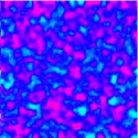
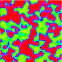
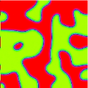
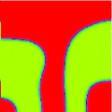
$\tilde{b}$

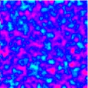
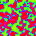
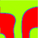
Figure 1: Simulation 1. Starting from a homogeneous racemic condition, the local random fluctuations induced by imperfect mixing drive the system to a homochiral solution. Time runs from left to right. See the text for details.

$\tilde{a}$
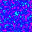
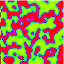
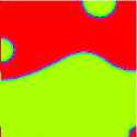
$\tilde{b}$

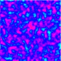
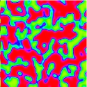
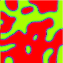
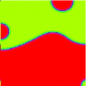
Figure 2: Simulation 2. The system is solved again with the same conditions as in Fig. 2. The new random fluctuations induced by imperfect mixing lead the system to a different final state with spatial segregation. Time runs from left to right.

We verified that the complex solutions of Eqs.(13,14), once averaged over the fluctuations, do indeed yield real results, in accord with the theoretical expectations [13]. Next, we evaluate the time evolution of the spatially averaged (over $\hat{x},\hat{y}$) densities for the two cases shown above and for two other simulations representative of the inverse situation (i.e., where the system is dominated by the other enantiomer). We represent in Fig. 3 the time evolution of the averaged enantiomeric excess $ee(\tau)=\frac{<\tilde{a}>-<\tilde{b}>}{<\tilde{a}>+<\tilde{b}>}$. When the solution is spatially homogeneous with $\tilde{a}$ at its maximal value, then $ee=+1$, for the inverse situation where $\tilde{b}$ is amplified maximally, then $ee=-1$, whereas for the intermediate situation with spatial compartmentalization $0<ee<1$ if the region with $\tilde{a}$ is greater than the one with $\tilde{b}$, and $-1<ee<0$ for the opposite situation. All these outcomes were found with roughly equal probability over the total of the 20 numerical simulations performed.

As for the evolution of a system with $g=\frac{0.14}{0.09}=1.555>1$ the system converges to the homogeneous solution $\tilde{a}=\tilde{b}=1/(1+g)$ with small fluctuations about this value, i.e. the racemic state (III). All the results shown appear for a wide range of fluctuation intensities ($\epsilon=10^{-2}-10^{-6}$).

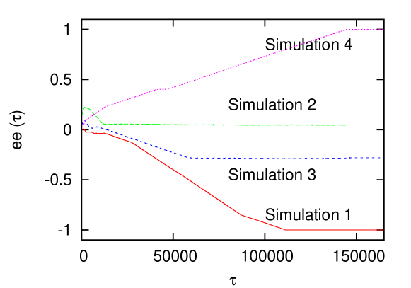
Figure 3: Time evolution of the spatially averaged enantiomeric excess $ee(\tau)=\frac{<\tilde{a}>-<\tilde{b}>}{<\tilde{a}>+<\tilde{b}>}$ of four representative simulations of the same study case, starting from racemic conditions (not resolvable in the figure). Due to the inherent symmetry of the reaction, either enantiomer $\tilde{a}$ or $\tilde{b}$ can dominate. The final result varies from one simulation to another. One can have total, homogeneous, chiral amplification (Simulations 1 and 4) or local chiral amplification with a racemic front (Simulations 2 and 3).

5 Conclusions

Internal particle density fluctuations automatically and inevitably lead to chiral symmetry breaking in an extension [7, 6] of the Frank model. The inclusion of this noise is carried out through a first-principles technique which allows us to map the chemical master equation to the corresponding coarse-grained Langevin equations. This multiplicative noise is rigorously determined by this procedure and is not an ad-hoc addition to the mean field equations. A marked advantage of the fully stochastic model is that no initial chiral seed nor external chiral field [15] are needed: full homochirality is achieved starting from a strictly racemic initial condition. In the limit as $\epsilon\rightarrow 0$, we would likely be sensitive to round-off errors, which also seem to induce chiral symmetry breaking, as reported in [16]. In two dimensions, there is a second class of solutions (see Simulation 2 in Fig. 2) for which the final state consists of two enantiomeric pure regions separated by a racemic interface or boundary. Regarding the solutions displayed in Figs 1 and 2, it is amusing to point out that Frank, in conceiving of what may be expected to happen in imperfectly mixed systems, predicted the formation of separate “colonies” of the two kinds of enantiomers bounded by racemic surfaces, with chiral homogeneity maintained within each such colony. He also stated that any initial curvature in these boundaries makes the boundary move towards the side from which it is concave, a feature which we have also observed in our simulations. The consequence of this is that any enclave of the one species will eventually shrink, and the other survives; this is what we observe in simulations of type 1 (see Fig 1). An exception to this rule occurs “when the two seas are connected by a strait. A different species could survive in each sea, with the (racemic) boundary running stably from cape to cape” [4]. This is indeed what happens in simulations of type 2 (see Fig.2)

An entirely different stochastic version of the Frank model was presented in [17]. Chiral amplification is also achieved starting from a racemic initial state. There the noise is incorporated in an ad-hoc fashion by assuming fluctuating kinetic constants $k_{i}$.

We thank Dr. Vladik Avetisov for his interest in this work, as well as Prof. Albert Moyano, and Prof. Josep M. Ribó for useful discussions and comments. M.-P. Z. is supported by the INTA and the research of D.H. is supported in part by funds from CSIC and INTA.

References

- [1] V. Avetisov and V. Goldanskii, Proc. Natl. Acad. Sci. USA 93 (1996)11435.
- [2] M. Avalos, R. Babiano, P. Cintas, J.L. Jiménez and J.C. Palacios, Tetrahedron Asymm. 11 (2000) 2845.
- [3] D.K. Kondepudi and K. Asakura, Acc. Chem. Res. 34 (2001) 946.
- [4] F.C. Frank, Biochim. et Biophys. Acta 11 (1953) 459.
- [5] I.R. Epstein, Nature 374 (1995) 321.
- [6] I. Gutman, D. Todorović and M. Vučković, Chem. Phys. Lett. 216 (1993) 447.
- [7] S.F. Mason, Nature 314 (1985) 400.
- [8] T. Buhse, J. Mex. Chem. Soc. 49(4) (2005) 328.
- [9] M. Doi, J. Phys. A: Math. Gen. 9 (1976) 1479.
- [10] L. Peliti, J. Physique 46 (1985) 1469.
- [11] For a recent review of these methods, see e.g., U.C. Täuber, M. Howard and B.P. Volmayr-Lee, J. Phys. A: Math. Gen. 38 (2005) R79.
- [12] D.J. Amit, Field Theory, the Renormalization Group, and Critical Phenomena, McGraw-Hill, New York, 1978.
- [13] M.J. Howard and U.C. Täuber, J. Phys. A:Math. Gen. 30 (1997) 7721.
- [14] D. Hochberg, M.-P. Zorzano and F, Morán, Phys. Rev. E 73 (2006) 066109.
- [15] M. Avalos, R. Babiano, P. Cintas, J.L. Jiménez, J.C. Palacios and L.D. Barron, Chem. Rev. 98 (1998) 2391.
- [16] J. Rivera Islas, D. Lavabre, J.-M. Grevy, R. Hernández Lamoneda, H. Rojas Cabrera, J.-C. Micheau and T. Buhse, Proc. Natl. Acad. Sci. USA 102 (2005) 13743.
- [17] D. Todorović, I. Gutman and M. Radulović, Chem. Phys. Lett. 372 (2003) 464.