The micromechanics of fluid-solid interactions during growth in porous soft biological tissue

Abstract

In this paper we address some modelling issues related to biological growth. Our treatment is based on a recently-proposed, general formulation for growth within the context of Mixture Theory (Journal of the Mechanics and Physics of Solids, 52, 2004, 1595–1625). We aim to enhance this treatment by making it more appropriate for the biophysics of growth in porous soft tissue, specifically tendon. This involves several modifications to the mathematical formulation to represent the reactions, transport and mechanics, and their interactions. We also reformulate the governing differential equations for reaction-transport to represent the incompressibility constraint on the fluid phase of the tissue. This revision enables a straightforward implementation of numerical stabilisation for the hyperbolic, or advection-dominated, limit. A finite element implementation employing an operator splitting scheme is used to solve the coupled, non-linear partial differential equations that arise from the theory. Motivated by our experimental model, an in vitro scaffold-free engineered tendon formed by self-assembly of tendon fibroblasts (Tissue Engineering, 10, 2004, 755–761), we solve several numerical examples demonstrating biophysical aspects of tissue growth, and the improved numerical performance of the models.

1 Introduction

Growth involves the addition or depletion of mass in biological tissue. Growth occurs in combination with remodelling, which is a change in microstructure, and possibly with morphogenesis, which is a change in form in the embryonic state. The physics of these processes are quite distinct, and for modelling purposes can, and must, be separated. Our previous work (Garikipati et al., 2004), upon which we now seek to build, drew in some measure from Cowin and Hegedus (1976); Epstein and Maugin (2000), and Taber and Humphrey (2001), and was focused upon a comprehensive account of the coupling between transport and mechanics. The origins of this coupling were traced to the balance equations, kinematics and constitutive relations. A major contribution of that work was the identification and discussion of several driving forces for transport that are thermodynamically-consistent, in the sense that specification of these relations does not violate the Clausius-Duhem dissipation inequality.

There have been a number of significant papers on biological growth and remodelling in the last 7–8 years of which we touch upon some, whose approaches are either similar to ours in some respects or differ in important ways. Humphrey and Rajagopal (2002) provided a mathematical treatment of adaptation in a tissue, which includes growth and remodelling in the sense of this paper. The authors identified adaptation as perhaps the most important mechanical characteristic of biological tissue. They introduced the notion of evolving natural configurations to model the state of material deposited at different instants in time. The treatment of the growth part of the deformation gradient in this paper bears some resemblance to this idea, although a detailed development has not been pursued here. The focus, instead, is on detailing some aspects of the problem that derive from treatment of the tissue as a porous medium, or as a mixture of interacting species. Preziosi and Farina (2002) developed an extension to the classical Darcy’s Law to incorporate mass exchanges between reacting species. This consideration is relevant to growth problems; however, in our opinion, these issues were subsumed in Garikipati et al. (2004), upon which this paper is based. Many of the ideas employed here are applicable to tumour growth problems; however, due to our current focus on tendon, we do not include phenomena such as angiogenesis and cell migration (see for example Breward et al., 2003). The changes in concentration that occur with growth tend to cause swelling or contraction of the tissue. This phenomenon has been accounted for previously by us in fields unrelated to Biology, using the idea of thermal expansion. See, for example, Rao et al. (2000) and Garikipati et al. (2001), which, too, are probably not the first instances of this idea. In the literature on biological growth this connection was made by Klisch and Hoger (2003).

In the present paper, we seek to restrict the range of physically-admissible models in order to gain greater physiological relevance for modelling growth in soft biological tissue. We also include one improvement in the mathematical/numerical treatment: The advection-diffusion equations for mass transport require numerical stabilisation in the advection-dominated regime (the hyperbolic limit). We draw upon the enforcement of the incompressibility limit for the fluid phase to facilitate this development. Below, we briefly introduce each aspect that we have considered, but postpone details until relevant sections in the paper.

• For a tissue undergoing finite strain, the transport equations can be formulated, mathematically, in terms of concentrations with respect to either the reference or current (deformed) configuration. However, the physics of fluid-tissue interactions and the imposition of relevant boundary conditions is best understood and represented in the current configuration.

• The state of saturation is crucial in determining whether the tissue swells or shrinks with infusion/expulsion of fluid. This aspect has been introduced into the formulation.

• The fluid phase, whether slightly compressible or incompressible, can develop compressive stress without bound. However, it can develop at most a small tensile stress (Brennen, 1995), having implications for the stiffness of the tissue in tension as against compression. Although this also has implications for void formation through cavitation, the ambient pressure in the tissue under normal physiological conditions ensures that this manifests itself only as a reduction in compressive pressure.

• When modelling transport, it is common to assume Fickean diffusion (Kuhl and Steinmann, 2003). This implies the existence of a mixing entropy due to the configurations available to molecules of the diffusing species at fixed values of the macroscopic concentration. The state of fluid saturation directly influences its mixing entropy.

• If fluid saturation is maintained, void formation in the pores is disallowed even under an increase in the pores’ volume. This has implications for the fluid exchanges between a deforming tissue and a fluid bath with which it is in contact.

• Recognising the incompressibility of the fluid phase, it is common to treat soft biological tissue as either incompressible or nearly-incompressible (Fung, 1993). At the scale of the pores (the microscopic scale in this case), however, a distinction exists in that the fluid is exactly (or nearly) incompressible, while the porous solid network is not obviously incompressible.

• In Garikipati et al. (2004), the acceleration of the solid phase was included as a driving force in the constitutive relation for the flux of other phases. However, acceleration is not frame-invariant and its use in constitutive relations is inappropriate.

• Chemical solutes in the extra-cellular fluid are advected by the fluid velocity and additionally undergo transport under a chemical potential gradient relative to the fluid. In the hyperbolic limit, where advection dominates, spatial instabilities emerge in numerical solutions of these transport equations (Brooks and Hughes, 1982; Hughes et al., 1987). Numerical stabilisation of the equations is intimately tied to the mathematical representation of fluid incompressibility.

• The modelling of solid-fluid mechanical coupling carries strong implications for the stiffness of tissue response, the nature of fluid transport, and since nutrients are dissolved in the fluid, ultimately for growth. We present upper and lower bounds for this problem and computations of coupled boundary value problems with these bounds.

These issues are treated in detail in relevant sections of the paper, which is laid out as follows: Balance equations and kinematics are discussed in Section 2, constitutive relations for reactions, transport and mechanics in Section 3, and numerical examples are presented in Section 4. Conclusions are drawn in Section 5.

2 Balance equations and kinematics of growth

In this section, the coupled, continuum balance equations governing the behaviour of growing tissue are summarised and specialised as outlined in Section 1. For detailed continuum mechanical arguments underlying the equations, the interested reader is directed to Garikipati et al. (2004).

The tissue of interest is an open subset of $\mathbb{R}^{3}$ with a piecewise smooth boundary. At a reference placement of the tissue, $\Omega_{0}$, points in the tissue are identified by their reference positions, $\mbox{\boldmath$X$}\in\Omega_{0}$. The motion of the tissue is a sufficiently smooth bijective map $\mbox{\boldmath$\varphi$}:\overline{\Omega}_{0}\times[0,T]\rightarrow\mathbb{R}^{3}$, where $\overline{\Omega}_{0}:=\Omega_{0}\cup\partial\Omega_{0}$; $\partial\Omega_{0}$ being the boundary of $\Omega_{0}$. At a typical time $t\in[0,T]$, $\mbox{\boldmath$\varphi$}(\mbox{\boldmath$X$},t)$ maps a point $X$ to its current position, $x$. In its current configuration, the tissue occupies a region $\Omega_{t}=\mbox{\boldmath$\varphi$}_{t}(\Omega_{0})$. These details are depicted in Figure 1. The deformation gradient $\mbox{\boldmath$F$}:=\partial\mbox{\boldmath$\varphi$}/\partial\mbox{\boldmath$X$}$ is the tangent map of $\varphi$.

\psfrag{A}{\small$\mbox{\boldmath$X$}$}\psfrag{F}{\small$\mbox{\boldmath$x$}$}\psfrag{B}{\small$\Pi^{\iota}$}\psfrag{G}{\small$\pi^{\iota}$}\psfrag{E}{\small$\mbox{\boldmath$\varphi$}$}\psfrag{C}{\small$\Omega_{0}$}\psfrag{H}{\small$\Omega_{t}$}\psfrag{D}{\small$\mbox{\boldmath$N$}\cdot\mbox{\boldmath$M$}^{\iota}$}\psfrag{I}{\small$\mbox{\boldmath$n$}\cdot\mbox{\boldmath$m$}^{\iota}$}\includegraphics[width=213.39566pt]{cp-mass-solute.eps}

Figure 1: The tissue as a continuous medium with growing and diffusing species.

The tissue consists of numerous species, of which the following groupings are of importance for the models: A solid species, consisting of solid collagen fibrils and cells, denoted by $\mathrm{c}$, an extra-cellular fluid species denoted by $\mathrm{f}$ and consisting primarily of water, and solute species, consisting of precursors to reactions, byproducts, nutrients, and other regulatory chemicals. A generic solute will be denoted by $\mathrm{s}$. In what follows, an arbitrary species will be denoted by $\iota$, where $\iota=\mathrm{c,f,s}$.

The fundamental quantities of interest are mass concentrations, $\rho_{0}^{\iota}(\mbox{\boldmath$X$},t)$. These are the masses of each species per unit system volume in $\Omega_{0}$. Formally, these quantities can also be thought of in terms of the maps $\rho_{0}^{\iota}:\overline{\Omega}_{0}\times[0,T]\rightarrow\mathbb{R}$, upon which the formulation imposes some smoothness requirements. By definition, the total material density of the tissue at a point is a sum of these concentrations over all species $\sum\limits_{\iota}\rho_{0}^{\iota}=\rho_{0}$. Other than the solid species, $\mathrm{c}$, all phases have mass fluxes, $\mbox{\boldmath$M$}^{\iota}$. These are mass flow rates per unit cross-sectional area in the reference configuration defined relative to the solid phase. The species have mass sources (or sinks), $\Pi^{\iota}$.

2.1 Balance of mass for an open system

As a result of mass transport (via the flux terms) and inter-conversion of species (via the source/sink terms) introduced above, the concentrations, $\rho_{0}^{\iota}$, change with time. In local form, the balance of mass for an arbitrary species in the reference configuration is

$$\frac{\partial\rho_{0}^{\iota}}{\partial t}=\Pi^{\iota}-\mathrm{\small{DIV}}[\mbox{\boldmath$M$}^{\iota}],\;\forall\,\iota,$$ (1)

recalling that, in particular, $\mbox{\boldmath$M$}^{c}={\bf 0}$. Here, $\mathrm{\small{DIV}[\bullet]}$ is the divergence operator in the reference configuration. The functional forms of $\Pi^{\iota}$ are abstractions of the underlying biochemistry, physiologically relevant examples of which are discussed in Section 3.4, and the fluxes, $\mbox{\boldmath$M$}^{\iota}$, are determined from the thermodynamically-motivated constitutive relations described in Section 3.3.

The behaviour of the entire system can be determined by summing Equation (1) over all species $\iota$. Additionally, sources and sinks satisfy the relation

$$\sum\limits_{\iota}\Pi^{\iota}=0,$$ (2)

which is consistent (Garikipati et al., 2004) with the Law of Mass Action for reaction rates and with Mixture Theory (Truesdell and Noll, 1965).

2.1.1 The role of mass balance in the current configuration

In order to proceed, we must first introduce the central kinematic assumption underlying the formulation: We assume that the pore structure deforms with the collagenous phase. Therefore, the deformation gradient, $F$, is common to c and the fluid-filled pore spaces. Furthermore, in what follows, we will treat the fluid as ideal and nearly-incompressible, i.e. as elastic (Section 3.2). This combination of kinematic and constitutive assumptions to be elaborated upon, implies that the stress in the fluid phase is determined by the elastic part of $F$ (see Sections 2.2 and 3.2). For clarity we denote it as $\mbox{\boldmath$F$}^{\mathrm{e}^{\mathrm{f}}}$. Importantly, the pore-filling fluid under stress can also undergo transport relative to the pore network; i.e., relative to the collagenous phase. This is the fluid flux, denoted by $\mbox{\boldmath$M$}^{\mathrm{f}}$ in the reference configuration. Note that the specification of constitutive relations for the flux is still open at this point in the discussion. At the outset, we preclude stress in any of the solute species, s. Only the solid collagen and fluid bear stress.

Although the initial/boundary value problem of mass transport can be consistently posed in the reference configuration, the evolving current configuration, $\Omega_{t}$, is of greater interest from a physical standpoint for growth problems. It follows from the discussion in the preceding paragraph that the shape and size of pores in $\Omega_{t}$ is determined by $F$. Therefore, at the boundary, the fluid concentration with respect to $\Omega_{t}$ remains constant if the boundary is in contact with a fluid bath. Accordingly, this is the appropriate Dirichlet boundary condition to impose under normal physiological conditions. This is shown in an idealised manner in Figure 2.

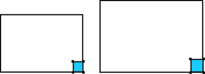
Figure 2: If the pore structure at the boundary deforms with the tissue and this boundary is in contact with a fluid bath, the fluid concentration with respect to the current configuration, i.e., $\rho^{\mathrm{f}}$, remains constant.

In the interest of applying boundary conditions (either specification of species flux or concentration) that are physically meaningful, we use the local form of the balance of mass in the current configuration,

$$\frac{\mathrm{d}\rho^{\iota}}{\mathrm{d}t}=\pi^{\iota}-\mathrm{\small{div}}[\mbox{\boldmath$m$}^{\iota}]-\rho^{\iota}\mathrm{\small{div}}[\mbox{\boldmath$v$}],\;\forall\,\iota,$$ (3)

where $\rho^{\iota}(\mbox{\boldmath$x$},t),\pi^{\iota}(\mbox{\boldmath$x$},t)$, and $\mbox{\boldmath$m$}^{\iota}(\mbox{\boldmath$x$},t)$ are the current mass concentration, source and mass flux of species $\iota$ respectively and $\mbox{\boldmath$v$}(\mbox{\boldmath$x$},t)$ is the velocity of the solid phase. They are related to corresponding reference quantities as $\rho^{\iota}=\left(\mathrm{det}\left(\mbox{\boldmath$F$}\right)\right)^{-1}\rho_{0}^{\iota}$, $\pi^{\iota}=\left(\mathrm{det}\left(\mbox{\boldmath$F$}\right)\right)^{-1}\Pi^{\iota}$ and $\mbox{\boldmath$m$}^{\iota}=\left(\mathrm{det}\left(\mbox{\boldmath$F$}\right)\right)^{-1}\mbox{\boldmath$F$}\mbox{\boldmath$M$}^{\iota}$. The spatial divergence operator is div [•], and the left hand-side in Equation (3) is the material time derivative relative to the solid, which may be written explicitly as $\frac{\partial}{\partial t}|_{X}$, implying that the reference position of the solid collagenous skeleton is held fixed.

2.2 The kinematics of growth induced by changes in concentration

\psfrag{A}{\small$\Omega_{0}$}\psfrag{B}{\small$\Omega^{\ast}$}\psfrag{C}{\small$\Omega_{t}$}\psfrag{D}{\small$\mbox{\boldmath$X$}$}\psfrag{E}{\small$\mbox{\boldmath$X$}^{\ast}$}\psfrag{F}{\small$\mbox{\boldmath$x$}$}\psfrag{G}{\small$\mbox{\boldmath$F$}^{\mathrm{g}^{\mathrm{\iota}}}$}\psfrag{H}{\small$\widetilde{\mbox{\boldmath$F$}}^{\mathrm{e}^{\mathrm{\iota}}}$}\psfrag{I}{\small$\widetilde{\mbox{\boldmath$F$}}$}\psfrag{J}{\small$\overline{\mbox{\boldmath$F$}}^{\mathrm{e}}$}\psfrag{K}{\small$\mbox{\boldmath$F$}$}\psfrag{L}{\small$\mbox{\boldmath$\kappa$}$}\psfrag{M}{\small$\mbox{\boldmath$u$}^{\ast}$}\psfrag{N}{\small$\mbox{\boldmath$\varphi$}$}\includegraphics[width=213.39566pt]{kinematics.eps}

Figure 3: The kinematics of growth, which holds for $\iota=\mathrm{c,f}$.

Local volumetric changes are associated with changes in the concentrations of the solid collagen and fluid, $\iota=\mathrm{c,f}$. If the material of the solid collagen or fluid remains stress free, it swells with an increase in concentration (mass of the species per unit system volume), and shrinks as its concentration decreases. This leads to the notion of a growth deformation gradient. One aspect of the coupling between mass transport and mechanics stems from this phenomenon. In the setting of finite strain kinematics, the total deformation gradient, $F$, is decomposed into the growth component of the solid collagen, $\mbox{\boldmath$F$}^{\mathrm{g}^{\mathrm{c}}}$, a geometrically-necessitated elastic component accompanying growth, $\widetilde{\mbox{\boldmath$F$}}^{\mathrm{e}^{\mathrm{c}}}$ and an additional elastic component due to external stress, $\overline{\mbox{\boldmath$F$}}^{\mathrm{e}^{\mathrm{c}}}$. Later, we will write $\mbox{\boldmath$F$}^{\mathrm{e}^{\mathrm{c}}}=\overline{\mbox{\boldmath$F$}}^{\mathrm{e}^{\mathrm{c}}}\widetilde{\mbox{\boldmath$F$}}^{\mathrm{e}^{\mathrm{c}}}$. This split is analogous to the classical decomposition of multiplicative plasticity (Lee, 1969) and is similar to the approach followed in existing literature on biological growth (see for e.g. Klisch et al., 2001; Taber and Humphrey, 2001; Ambrosi and Mollica, 2002). As explained in Section 2.1.1, we assume that the fluid-filled pores also deform with $F$, and that a component, $\mbox{\boldmath$F$}^{\mathrm{e}^{\mathrm{f}}}$, of this total deformation gradient tensor, determines the fluid stress. We also assume a fluid growth component, $\mbox{\boldmath$F$}^{\mathrm{g}^{\mathrm{f}}}$, which we elaborate below, and that $\mbox{\boldmath$F$}^{\mathrm{e}^{\mathrm{f}}}\mbox{\boldmath$F$}^{\mathrm{g}^{\mathrm{f}}}=\mbox{\boldmath$F$}$. As with the solid collagen we admit $\mbox{\boldmath$F$}^{\mathrm{e}^{\mathrm{f}}}=\overline{\mbox{\boldmath$F$}}^{\mathrm{e}^{\mathrm{f}}}\widetilde{\mbox{\boldmath$F$}}^{\mathrm{e}^{\mathrm{f}}}$, the sub-components carrying the same interpretation as for the solid collagen. However, we do not explicitly use this last decomposition.

The elastic-growth decomposition is visualised in Figure 3. Assuming that the volume changes associated with growth described above are isotropic, a simple form for the growth part of the deformation gradient tensor is

$$\mbox{\boldmath$F$}^{\mathrm{g}^{\iota}}=\left(\frac{\rho_{0}^{\iota}}{\rho_{0_{\mathrm{ini}}}^{\iota}}\right)^{\frac{1}{3}}{\bf 1},\quad\iota=\mathrm{c,f}$$ (4)

where $\rho_{0_{\mathrm{ini}}}^{\iota}(\mbox{\boldmath$X$})$ is the reference concentration at the initial time, and 1 is the second-order isotropic tensor. In the state, $\mbox{\boldmath$F$}=\mbox{\boldmath$F$}^{\mathrm{g}^{\iota}}$, the species would be stress free. The kinematics being local, the action of $\mbox{\boldmath$F$}^{\mathrm{g}^{\iota}}$ alone can result in incompatibility, which is eliminated by the geometrically-necessary elastic deformation $\widetilde{\mbox{\boldmath$F$}}^{\mathrm{e}^{\mathrm{\iota}}}$, which causes an internal, self-equilibrated stress. The component $\overline{\mbox{\boldmath$F$}}^{\mathrm{e}^{\iota}}$ is associated with the external stress.

2.2.1 Saturation and tissue swelling

\psfrag{A}{\small A}\psfrag{B}{\small B}\psfrag{C}{\small B}\psfrag{D}{\small C}\psfrag{E}{\small Unsaturated}\psfrag{F}{\small Saturated}\includegraphics[width=213.39566pt]{composite.eps}

Figure 4: Unsaturated tissue in the current configuration (A) allows influx of fluid without swelling until it is completely saturated (B). Initially saturated tissue (B), in general, swells with influx of fluid (C).

The degree of saturation of the solid phase plays a fundamental role in determining whether the tissue responds to an infusion (expulsion) of fluid by swelling (shrinking). In particular, the isotropic swelling law defined by Equation (4) has to be generalised to treat the case in which the solid phase is not saturated by fluid.

Figure 4 schematically depicts two possible scenarios. If the tissue is unsaturated in its current configuration, as in A, then, on a microscopic scale, it contains unfilled voids. It is thus capable of allowing an influx of fluid, which tends to increase its degree of saturation until fully saturated, as in B. This increase does not cause swelling of the tissue in the local stress-free state, as there is free volume for incoming fluid to occupy. However, once the tissue is saturated in the current configuration, an increase in the fluid content causes swelling in the stress-free state, as depicted in C, since there is no free volume for the entering fluid to occupy. It is this second case that is modelled by (4). It is worth emphasizing that this argument holds for $\mbox{\boldmath$F$}^{\mathrm{g}^{\mathrm{f}}}$, which is the local stress-free state of deformation of the fluid-containing pores at a point. The actual deformation gradient, $\mbox{\boldmath$F$}=\mbox{\boldmath$F$}^{\mathrm{e}^{\mathrm{f}}}\mbox{\boldmath$F$}^{\mathrm{g}^{\mathrm{f}}}$, also depends on the the elastic part, $\mbox{\boldmath$F$}^{\mathrm{e}^{\mathrm{f}}}$, which is determined by the constitutive response of the fluid. Under stress, an incompressible fluid will have $\mathrm{det}\mbox{\boldmath$F$}^{\mathrm{e}^{\mathrm{f}}}=1$ and therefore a fluid-saturated tissue will swell with fluid influx, $\mathrm{det}\mbox{\boldmath$F$}=\mathrm{det}\mbox{\boldmath$F$}^{\mathrm{g}^{\mathrm{f}}}>1$. A compressible fluid may have $\mathrm{det}\mbox{\boldmath$F$}^{\mathrm{e}^{\mathrm{f}}}<1$ allowing $\mathrm{det}\mbox{\boldmath$F$}<1$ even with $\mathrm{det}\mbox{\boldmath$F$}^{\mathrm{g}^{\mathrm{f}}}>1$. Even in this case, however, in the stress-free state there will be swelling.

Therefore, for the fluid phase, the isotropic swelling law can be extended to the unsaturated case by introducing a degree of saturation, $\tilde{v}^{\iota}$, defined in the current configuration, $\Omega_{t}$. We have $\tilde{v}^{\iota}=\rho^{\iota}/\tilde{\rho}^{\iota}$, where $\tilde{\rho}^{\iota}$ is the intrinsic density in $\Omega_{t}$ and is given by $\tilde{\rho}^{\iota}=\tilde{\rho}^{\iota}_{0}/\mathrm{det}\mbox{\boldmath$F$}$. Note that the intrinsic reference density, $\tilde{\rho}^{\iota}_{0}$, is a material property. Upon solution of the mass balance equation (3) for $\rho^{\iota}$, the species volume fractions, $\tilde{v}^{\iota}$, can therefore be computed in a straightforward fashion. The sum of these volume fractions is our required measure of saturation defined in $\Omega_{t}$. Also, recognizing that for the dilute solutions obtained with physiologically-relevant solute concentrations, the saturation condition is very well approximated by $\tilde{v}^{\mathrm{f}}+\tilde{v}^{\mathrm{s}}=1$, we proceed to redefine the fluid growth-induced component of the pore deformation gradient tensor as follows:

$$\mbox{\boldmath$F$}^{\mathrm{g}^{\mathrm{f}}}=\left\{\begin{array}[]{ll}\left(\frac{\rho_{0}^{\mathrm{f}}}{\rho_{0_{\mathrm{sat}}}^{\mathrm{f}}}\right)^{\frac{1}{3}}{\bf 1},&\tilde{v}^{\mathrm{f}}+\tilde{v}^{\mathrm{s}}=1\\ {\bf 1},&\mathrm{otherwise.}\end{array}\right.$$ (5)

In (5) $\rho_{0_{\mathrm{sat}}}^{\mathrm{f}}$ is the reference concentration value at which the tissue attains saturation in the current configuration.

With this redefinition of $\mbox{\boldmath$F$}^{\mathrm{g}^{\mathrm{f}}}$ it is implicit that $\tilde{v}^{\mathrm{f}}+\tilde{v}^{\mathrm{s}}>1$ is non-physical. Saturation holds in the sense that $\tilde{v}^{\mathrm{f}}+\tilde{v}^{\mathrm{s}}=1$, and it actually allows $\sum_{\iota}\tilde{v}^{\iota}>1$ if the sum is over all species. It has been common in the soft tissue literature to assume that, under normal physiological conditions, soft tissues are fully saturated by the fluid and Equation (4) is appropriate for $\iota=\mathrm{f}$. However, this treatment of saturation and swelling induced by the fluid phase is necessary background for Section 3.2.1 where we discuss the response of the fluid phase under tension. This treatment also holds relevance for partial drying, which ex vivo or in vitro tissue may be subject to under certain laboratory conditions, and is central to the mechanics of drained porous media other than biological tissue, most prominently, soils.

2.3 Balance of momenta

In soft tissues, the species production rate and flux that appear on the right hand-side in Equations (1) and (3), are strongly dependent on the local state of stress. To correctly model this coupling, the balance of linear momentum should be solved to determine the local state of strain and stress.

The deformation of the tissue is characterised by the map $\mbox{\boldmath$\varphi$}(\mbox{\boldmath$X$},t)$. Recognising that, in tendons, the solid collagen fibrils and fibroblasts do not undergo mass transport, the material velocity of this species, $\mbox{\boldmath$V$}=\partial\mbox{\boldmath$\varphi$}/\partial t$, is used as the primitive variable for mechanics. Each remaining species can undergo mass transport relative to the solid collagen. For this purpose, it is useful to define the material velocity of a species $\iota$ relative to the solid skeleton as: $\mbox{\boldmath$V$}^{\iota}=(1/\rho_{0}^{\iota})\mbox{\boldmath$F$}\mbox{\boldmath$M$}^{\iota}$. Thus, the total material velocity of a species $\iota$ is $\mbox{\boldmath$V$}+\mbox{\boldmath$V$}^{\iota}$.

The total first Piola-Kirchhoff stress tensor, $P$, is the sum of the partial stresses $\mbox{\boldmath$P$}^{\,\iota}$ (borne by a species $\iota$) over all the species present. Recognizing that solutes in low concentrations, and do not bear appreciable stress, the partial stresses and momentum balance equation are defined only for the solid collagen and fluid phases. With the introduction of these quantities, the balance of linear momentum in local form over $\Omega_{0}$ for solid collagen and fluid is,

$$\begin{split}\rho_{0}^{\iota}\frac{\partial}{\partial t}\left(\mbox{\boldmath$V$}+\mbox{\boldmath$V$}^{\iota}\right)&=\rho^{\iota}_{0}\left(\mbox{\boldmath$g$}+\mbox{\boldmath$q$}^{\iota}\right)+\mathrm{\small{DIV}}[\mbox{\boldmath$P$}^{\,\iota}]\\ &\quad-\left(\mathrm{\small{GRAD}}\left[\mbox{\boldmath$V$}+\mbox{\boldmath$V$}^{\iota}\right]\right)\mbox{\boldmath$M$}^{\iota},\quad\iota=\mathrm{c,f}\end{split}$$ (6)

where $g$ is the body force per unit mass, and $\mbox{\boldmath$q$}^{\iota}$ is an interaction term denoting the force per unit mass exerted upon $\iota$ by all other species present. The final term with the (reference) gradient denotes the contribution of the flux to the balance of momentum. In practise, the relative magnitude of the fluid mobility (and hence flux) is small, so the final term on the right hand side of Equation (6) is negligible, resulting in a more classical form of the balance of momentum. Furthermore, in the absence of significant acceleration of the tissue during growth, the left hand-side can also be neglected, reducing (6) to the quasi-static balance of linear momentum.

The balance of momentum of the entire tissue is obtained by summing Equation (6) over $\iota=\mathrm{c,f}$. Additionally, recognising that the rate of change of momentum of the entire tissue is affected only by external agents and is independent of internal interactions, the following relation arises.

$$\sum\limits_{\iota=\mathrm{c}}^{\mathrm{f}}\left(\rho^{\iota}_{0}\mbox{\boldmath$q$}^{\iota}+\Pi^{\iota}\mbox{\boldmath$V$}^{\iota}\right)=0.$$ (7)

This is also consistent with Classical Mixture Theory (Truesdell and Noll, 1965). See Garikipati et al. (2004) for further details on balance of linear momentum, and the formulation of balance of angular momentum. We only note here that the latter principle leads to a symmetric partial Cauchy stress, $\mbox{\boldmath$\sigma$}^{\iota}$ for each species in contrast with the unsymmetric Cauchy stress of Epstein and Maugin (2000).

3 Constitutive framework and specific models

As is customary in field theories of continuum physics, the Clausius-Duhem inequality is obtained by multiplying the Entropy Inequality (the Second Law of Thermodynamics) by the temperature field, $\theta$, and subtracting it from the Balance of Energy (the First Law of Thermodynamics). We assume the Helmholtz free energy per unit mass of species $\iota$ to have the form: $\psi^{\iota}=\hat{\psi}^{\iota}(\mbox{\boldmath$F$}^{\mathrm{e}^{\iota}},\theta,\rho_{0}^{\iota})$. Substituting this in the Clausius-Duhem inequality results in a form of this inequality that the specified constitutive relations must not violate. Only the valid constitutive laws relevant to the examples that follow are listed here. For details, see Garikipati et al. (2004).

3.1 An anisotropic network model based on entropic elasticity

The partial first Piola-Kirchhoff stress of collagen, modelled as a hyperelastic material, is $\mbox{\boldmath$P$}^{\,\mathrm{c}}=\rho_{0}^{\mathrm{c}}\partial\psi^{\mathrm{c}}/\partial\mbox{\boldmath$F$}^{\mathrm{e}^{\mathrm{c}}}$. Recall that $\mbox{\boldmath$F$}^{\mathrm{e}^{\mathrm{c}}}=\mbox{\boldmath$F$}\mbox{\boldmath$F$}^{\mathrm{g}^{\mathrm{c}^{-1}}}$ is the elastic part, and $\mbox{\boldmath$F$}^{\mathrm{g}^{\mathrm{c}}}$ is the growth part, respectively, of the deformation gradient, of collagen. Following Equation (4), if we were considering unidirectional growth of collagen along a unit vector $e$, we would have $\mbox{\boldmath$F$}^{\mathrm{g}^{\mathrm{c}}}=\frac{\rho^{\mathrm{c}}_{0}}{\rho^{\mathrm{c}}_{0_{\mathrm{ini}}}}\mbox{\boldmath$e$}\otimes\mbox{\boldmath$e$}$, with $\rho^{\mathrm{c}}_{0_{\mathrm{ini}}}$ denoting the initial concentration of collagen at the point.

The mechanical response of tendons in tension is determined primarily by their dominant structural component: highly oriented fibrils of collagen. In our preliminary formulation, the strain energy density for collagen has been obtained from hierarchical multi-scale considerations based upon an entropic elasticity-based worm-like chain (WLC) model (Kratky and Porod, 1949). The WLC model has been widely used for long chain single molecules, most prominently for DNA (Marko and Siggia, 1995; Rief et al., 1997; Bustamante et al., 2003), and recently for the collagen monomer (Sun et al., 2002). The central parameters of this model are the chain’s contour length, $L$, and persistence length, $A$. The latter is a measure of its stiffness and given by $A=\chi/k\theta$, where $\chi$ is the bending rigidity, $k$ is Boltzmann’s constant and $\theta$ is the temperature. See Landau and Lifshitz (1951) for general formulation of statistical mechanics models of long chain molecules.

To model a collagen network structure, the WLC model has been embedded as a single constituent chain of an eight-chain model (Bischoff et al., 2002a, b), depicted in Figure 5. Homogenisation via averaging then leads to a continuum Helmholtz free energy function, $\hat{\psi}^{\mathrm{c}}$:

$$\begin{split}\rho^{\mathrm{c}}_{0}\hat{\psi}^{\mathrm{c}}(\mbox{\boldmath$F$}^{\mathrm{e}^{\mathrm{c}}},\rho^{\mathrm{c}}_{0})&=\frac{Nk\theta}{4A}\left(\frac{r^{2}}{2L}+\frac{L}{4(1-r/L)}-\frac{r}{4}\right)\\ &+\frac{\gamma}{\beta}({J^{\mathrm{e}^{\mathrm{c}^{-2\beta}}}}-1)+\gamma{\bf 1}\colon(\mbox{\boldmath$C$}^{\mathrm{e}^{\mathrm{c}}}-{\bf 1})\\ &-\frac{Nk\theta}{4\sqrt{2L/A}}\left(\sqrt{\frac{2A}{L}}+\frac{1}{4(1-\sqrt{2A/L})}-\frac{1}{4}\right)Z,\\ Z&=\log\left(\lambda_{1}^{{\mathrm{e}}^{a^{\mathrm{2}}}}\lambda_{2}^{{\mathrm{e}}^{b^{\mathrm{2}}}}\lambda_{3}^{{\mathrm{e}}^{c^{\mathrm{2}}}}\right).\end{split}$$ (8)

Here, $N$ is the density of chains, and $a,b$ and $c$ are lengths of the unit cell sides aligned with the principal stretch directions. The material model is isotropic only if $a=b=c$.

\psfrag{r}{\small$r$}\psfrag{A}{\small$A$}\psfrag{a}{\small$a$}\psfrag{b}{\small$b$}\psfrag{c}{\small$c$}\psfrag{n}{\small$\mbox{\boldmath$N$}_{1}$}\psfrag{o}{\small$\mbox{\boldmath$N$}_{2}$}\psfrag{p}{\small$\mbox{\boldmath$N$}_{3}$}\includegraphics[width=213.39566pt]{wlcm-cuboid.eps}

Figure 5: The eight-chain model incorporating worm-like chains.

The elastic stretches along the unit cell axes are, respectively, denoted by $\lambda_{1}^{\mathrm{e}},\lambda_{2}^{\mathrm{e}}$ and $\lambda_{3}^{\mathrm{e}}$, $\mbox{\boldmath$C$}^{\mathrm{e}^{\mathrm{c}}}=\mbox{\boldmath$F$}^{\mathrm{e}^{\mathrm{c}^{\mathrm{T}}}}\mbox{\boldmath$F$}^{\mathrm{e}^{\mathrm{c}}}$ is the elastic right Cauchy-Green tensor of collagen. The factors $\gamma$ and $\beta$ control the bulk compressibility of the model. The end to end chain length is given by $r=\frac{1}{2}\sqrt{a^{2}\lambda_{1}^{\mathrm{e}^{2}}+b^{2}\lambda_{2}^{\mathrm{e}^{2}}+c^{2}\lambda_{3}^{\mathrm{e}^{2}}}$, where $\lambda^{\mathrm{e}}_{I}=\sqrt{\mbox{\boldmath$N$}_{I}\cdot\mbox{\boldmath$C$}^{\mathrm{e}^{\mathrm{c}}}\mbox{\boldmath$N$}_{I}}$, and $\mbox{\boldmath$N$}_{I},\,I=1,2,3$ are the unit vectors along the three unit cell axes, respectively. In our numerical simulations that appear below in Section 4, the numerical values used for the parameters introduced in (8) are based on those in Kuhl et al. (2005).

3.2 A nearly incompressible ideal fluid

In this preliminary work, the fluid phase is treated as nearly incompressible and ideal, i.e., inviscid. The partial Cauchy stress in the fluid is

$$\mbox{\boldmath$\sigma$}^{\mathrm{f}}=\mathrm{det}(\mbox{\boldmath$F$}^{\mathrm{e}^{\mathrm{f}}})^{-1}\mbox{\boldmath$P$}^{\,\mathrm{f}}\mbox{\boldmath$F$}^{\mathrm{e}^{\mathrm{fT}}}=h(\rho^{\mathrm{f}}){\bf 1},$$ (9)

where a large value of $h^{\prime}(\rho^{\mathrm{f}})$ ensures near-incompressibility.

3.2.1 Response of the fluid in tension; cavitation

The response of the ideal fluid, as defined by Equation (9), does not distinguish between tension and compression, i.e., whether $\mathrm{det}(\mbox{\boldmath$F$}^{\mathrm{e}^{\mathrm{f}}})\gtreqless 1$. Being (nearly) incompressible, the fluid can develop compressive hydrostatic stress without bound—a case that is modelled accurately. However, the fluid can develop at most a small tensile hydrostatic stress (Brennen, 1995), and the tensile stiffness is mainly from the collagen phase. This is not accurately represented by (9), which models a symmetric response in tension and compression.

Here, we preclude all tensile load carrying by the fluid by limiting $\mathrm{det}(\mbox{\boldmath$F$}^{\mathrm{e}^{\mathrm{f}}})\leq 1$. We first introduce an additional component to the relation between deformation of the pore space, given by $F$, the fluid stress-determining tensor, $\mbox{\boldmath$F$}^{\mathrm{e}^{\mathrm{f}}}$ and the growth tensor for the fluid, $\mbox{\boldmath$F$}^{\mathrm{g}^{\mathrm{f}}}$. Consider the cavitation (void forming) tensor, $\mbox{\boldmath$F$}^{\mathrm{v}}$, defined by

$$\mbox{\boldmath$F$}^{\mathrm{e}^{\mathrm{f}}}\mbox{\boldmath$F$}^{\mathrm{g}^{\mathrm{f}}}\mbox{\boldmath$F$}^{\mathrm{v}}=\mbox{\boldmath$F$}.$$ (10)

We restrict the formulation to include only saturated current configurations at $t=0$. Following Section 2.2.1 we have $\tilde{v}^{\mathrm{f}}+\tilde{v}^{\mathrm{c}}=1$ at $t=0$, the saturation condition in $\Omega_{t}$ when solutes are at low concentrations. At times $t>0$ Equation (5) holds for $\mbox{\boldmath$F$}^{\mathrm{g}^{\mathrm{f}}}$. If $\mathrm{det}[\mbox{\boldmath$F$}(\mbox{\boldmath$F$}^{\mathrm{g}^{\mathrm{f}}})^{-1}]\leq 1$ we set $\mbox{\boldmath$F$}^{\mathrm{e}^{\mathrm{f}}}=\mbox{\boldmath$F$}(\mbox{\boldmath$F$}^{\mathrm{g}^{\mathrm{f}}})^{-1}$ and $\mbox{\boldmath$F$}^{\mathrm{v}}={\bf 1}$ for no cavitation. Otherwise, since $\mathrm{det}[\mbox{\boldmath$F$}(\mbox{\boldmath$F$}^{\mathrm{g}^{\mathrm{f}}})^{-1}]>1$, we specify $\mbox{\boldmath$F$}^{\mathrm{e}^{\mathrm{f}}}=\mathrm{det}[\mbox{\boldmath$F$}(\mbox{\boldmath$F$}^{\mathrm{g}^{\mathrm{f}}})^{-1}]^{-1/3}\mbox{\boldmath$F$}(\mbox{\boldmath$F$}^{\mathrm{g}^{\mathrm{f}}})^{-1}$ thus restricting $\mbox{\boldmath$F$}^{\mathrm{e}^{\mathrm{f}}}$ to be unimodular and allow cavitation by writing $\mbox{\boldmath$F$}^{\mathrm{v}}=\mbox{\boldmath$F$}(\mbox{\boldmath$F$}^{\mathrm{e}^{\mathrm{f}}}\mbox{\boldmath$F$}^{\mathrm{g}^{\mathrm{f}}})^{-1}$. These conditional relations are summarized as

$$\mbox{\boldmath$F$}^{\mathrm{e}^{\mathrm{f}}}=\left\{\begin{array}[]{ll}\mbox{\boldmath$F$}(\mbox{\boldmath$F$}^{\mathrm{g}^{\mathrm{f}}})^{-1},\;\mbox{\boldmath$F$}^{\mathrm{v}}={\bf 1},&\mathrm{det}[\mbox{\boldmath$F$}(\mbox{\boldmath$F$}^{\mathrm{g}^{\mathrm{f}}})^{-1}]\leq 1\\ \mathrm{det}[\mbox{\boldmath$F$}(\mbox{\boldmath$F$}^{\mathrm{g}^{\mathrm{f}}})^{-1}]^{-1/3}\mbox{\boldmath$F$}(\mbox{\boldmath$F$}^{\mathrm{g}^{\mathrm{f}}})^{-1},&\\ \qquad\qquad\mbox{\boldmath$F$}^{\mathrm{v}}=\mbox{\boldmath$F$}(\mbox{\boldmath$F$}^{\mathrm{e}^{\mathrm{f}}}\mbox{\boldmath$F$}^{\mathrm{g}^{\mathrm{f}}})^{-1}&\mathrm{otherwise.}\end{array}\right.$$ (11)

3.3 Constitutive relations for fluxes

From Garikipati et al. (2004), the constitutive relation for the flux of extra-cellular fluid relative to collagen in the reference configuration takes the following form,

$$\mbox{\boldmath$M$}^{\mathrm{f}}=\mbox{\boldmath$D$}^{\mathrm{f}}\left(\rho_{0}^{\mathrm{f}}\mbox{\boldmath$F$}^{T}\mbox{\boldmath$g$}+\mbox{\boldmath$F$}^{T}\mathrm{\small{DIV}}\left[\mbox{\boldmath$P$}^{\,\mathrm{f}}\right]-\rho_{0}^{\mathrm{f}}\mathrm{\small{GRAD}}\mu^{\mathrm{f}}\right),$$ (12)

where $\mbox{\boldmath$D$}^{\mathrm{f}}$ is the positive semi-definite mobility of the fluid, and isothermal conditions are assumed in order to approximate the physiological ones. Experimentally determined transport coefficients (e.g. for mouse tail skin (Swartz et al., 1999) and rabbit Achilles tendons (Han et al., 2000)) are used for the fluid mobility values. The terms in the parenthesis on the right hand-side of Equation (12) sum to give the total driving force for transport. The first term is the contribution due to gravitational acceleration. In order to maintain physiological relevance, this term has been neglected in the following treatment. The second term arises from stress divergence; for an ideal fluid, it reduces to a pressure gradient, thereby specifying that the fluid moves down a compressive pressure gradient, which is Darcy’s Law. The third term is the gradient of the chemical potential, $\mu^{\mathrm{f}}=e^{\mathrm{f}}-\theta\eta^{\mathrm{f}}$, where $e^{\mathrm{f}}$ is the mass-specific internal energy, $\theta$ is temperature and $\eta^{\mathrm{f}}$ is the mass-specific entropy. The entropy gradient included in this term results in classical Fickean diffusion if only mixing entropy exists, as discussed in the following section. For a detailed derivation and discussion of Equation (12), the reader is directed to Garikipati et al. (2004).

3.3.1 Saturation and Fickean diffusion of the fluid

\psfrag{A}{\small A}\psfrag{B}{\small B}\psfrag{C}{\small C}\psfrag{D}{\small Vacant space}\psfrag{E}{\small Filled space}\includegraphics[width=213.39566pt]{saturation.eps}

Figure 6: Depicted at a microscopic scale, only unsaturated tissues A and B can undergo Fickean diffusion of the fluid. C is saturated.

As depicted in Figure 6, only when pores are unsaturated are there multiple configurations available to the fluid molecules at a fixed fluid concentration. This leads to a non-zero mixing entropy. In contrast, if saturated, there is a single available configuration (degeneracy), resulting in zero mixing entropy. Consequently, Fickean diffusion, which arises from the gradient of mixing entropy can exist only in the unsaturated case. However, even a saturated pore structure can demonstrate concentration gradient-dependent mass transport phenomenologically: The fluid stress depends on fluid concentration (see Equation (9)), and fluid stress gradient-driven flux appears as a concentration gradient-driven flux.

The saturation dependence of Fickean diffusion is modelled by using the measure of saturation introduced in Section 2.2.1. We rewrite the chemical potential as

$$\mu^{\mathrm{f}} = e^{\mathrm{f}}-\theta\eta^{\mathrm{f}},$$

$$\eta^{\mathrm{f}} \to 0,\quad\mbox{as}\,\tilde{v}^{\mathrm{f}}+\tilde{v}^{\mathrm{c}}\to 1.$$ (13)

It is again important to note that under physiological conditions, soft tissues are fully saturated by fluid, and it is appropriate to set $\mu^{\mathrm{f}}=e^{\mathrm{f}}$.

3.3.2 Transport of solute species

The dissolved solute species, denoted by s, undergo long range transport primarily by being advected by the fluid. In addition to this, they undergo diffusive transport relative to the fluid. This motivates an additional velocity split of the form $\mbox{\boldmath$V$}^{s}=\widetilde{\mbox{\boldmath$V$}^{\mathrm{s}}}+\mbox{\boldmath$V$}^{\mathrm{f}}$, where $\widetilde{\mbox{\boldmath$V$}^{\mathrm{s}}}$ denotes the velocity of the solute relative to the fluid. The constitutive relation for the corresponding flux, denoted by $\widetilde{\mbox{\boldmath$M$}^{s}}$, has the following form, similar to Equation (12) defined for the fluid flux.

$$\widetilde{\mbox{\boldmath$M$}^{\mathrm{s}}}=\mbox{\boldmath$D$}^{\mathrm{s}}\left(-\rho^{\mathrm{s}}_{0}\mathrm{\small{GRAD}}\left[e^{\mathrm{s}}-\theta\eta^{\mathrm{s}}\right]\right),$$ (14)

where $\mbox{\boldmath$D$}^{\mathrm{s}}$ is the positive semi-definite mobility of the solute relative to the fluid, and again, isothermal conditions are assumed to approximate the physiological ones. Following Section 2.3 there are no stress-dependent contributions to $\widetilde{\mbox{\boldmath$M$}^{\mathrm{s}}}$.

3.3.3 Frame invariance and the contribution from acceleration

In our earlier treatment (Garikipati et al., 2004), the constitutive relation for the fluid flux had a driving force contribution arising from the acceleration of the solid phase, $-\rho_{0}^{\mathrm{f}}\mbox{\boldmath$F$}^{\mathrm{T}}\frac{\partial\mbox{\boldmath$V$}}{\partial t}$. This term, being motivated by the reduced dissipation inequality, does not violate the Second Law and supports an intuitive understanding that the acceleration of the solid skeleton in one direction must result in an inertial driving force on the fluid in the opposite direction. However, as defined, this acceleration is obtained by the time differentiation of kinematic quantities, and does not transform in a frame-indifferent manner. Unlike the superficially similar term arising from the gravity vector, the acceleration term presents an improper dependence on the frame of the observer. Thus, its use in constitutive relations is inappropriate, and the term has been dropped in Equation (12).

3.3.4 Incompressible fluid in a porous solid

Upon incorporation of the additional velocity split, $\mbox{\boldmath$V$}^{\mathrm{s}}=\widetilde{\mbox{\boldmath$V$}^{\mathrm{s}}}+\mbox{\boldmath$V$}^{f}$, described in Section 3.3.2, the resulting mass transport equation (3) for the solute species is

$$\frac{\mathrm{d}\rho^{\mathrm{s}}}{\mathrm{d}t}=\pi^{\mathrm{s}}-\mathrm{div}\left[\widetilde{\mbox{\boldmath$m$}^{\mathrm{s}}}+\frac{\rho^{\mathrm{s}}}{\rho^{f}}\mbox{\boldmath$m$}^{f}\right]-\rho^{\mathrm{s}}\mathrm{div}[\mbox{\boldmath$v$}].$$ (15)

In the hyperbolic limit, where advection dominates, spatial oscillations emerge in numerical solutions of this equation (Brooks and Hughes, 1982; Hughes et al., 1987). However, the form in which the equation is obtained is not in standard advection-diffusion form, and therefore is not amenable to the application of standard stabilisation techniques (Hughes et al., 1987). In part, this is because although the (near) incompressibility of the fluid phase is embedded in the balance of linear momentum via the fluid stress, it has not yet been explicitly incorporated into the transport equations. This section proceeds to impose the fluid incompressibility condition and deduces implications for the solute mass transport equation, including a crucial simplification allowing for its straightforward numerical stabilisation.

From Equation (3), the local form of the balance of mass for the fluid species (recalling that $\Pi^{\mathrm{f}}=0$) in the current configuration is

$$\frac{\mathrm{d}\rho^{f}}{\mathrm{d}t}=-\mathrm{div}\left[\mbox{\boldmath$m$}^{f}\right]-\rho^{f}\mathrm{div}\left[\mbox{\boldmath$v$}\right].$$ (16)

In order to impose the incompressibility of the fluid, we first denote by $\rho_{0_{\mathrm{ini}}}^{f}$ the initial value of the fluid reference concentration. Recall that the fluid concentration with respect to the reference configuration evolves in time; $\rho^{\mathrm{f}}_{0}=\rho^{\mathrm{f}}_{0}(\mbox{\boldmath$X$},t)$. Therefore we can precisely, and non-trivially, define $\rho_{0_{\mathrm{ini}}}^{\mathrm{f}}(\mbox{\boldmath$X$})$

$$\begin{split}\rho_{0}^{\mathrm{f}}(\mbox{\boldmath$X$},0)&=:\rho_{0_{\mathrm{ini}}}^{\mathrm{f}}(\mbox{\boldmath$X$})\\ &=\rho_{\mathrm{ini}}^{\mathrm{f}}(\mbox{\boldmath$x$}\circ\mbox{\boldmath$\varphi$})J(\mbox{\boldmath$X$},t)\\ &=\frac{\rho^{\mathrm{f}}(\mbox{\boldmath$x$}\circ\mbox{\boldmath$\varphi$},t)}{J^{f_{\mathrm{g}}}(\mbox{\boldmath$X$},t)}J(\mbox{\boldmath$X$},t)\\ &=\rho^{\mathrm{f}}(\mbox{\boldmath$x$}\circ\mbox{\boldmath$\varphi$},t)\cancelto{\approx 1\ \forall\ t}{J^{f_{\mathrm{e}}}}(\mbox{\boldmath$X$},t).\\ \end{split}$$ (17)

In (LABEL:incompderiv), $J:=\mathrm{det}(\mbox{\boldmath$F$})$ and $J^{f_{\mathrm{g}}}:=\mathrm{det}(\mbox{\boldmath$F$}^{\mathrm{g}^{\mathrm{f}}})$. The quantity $\rho_{\mathrm{ini}}^{\mathrm{f}}$ is defined by the right hand-sides of the first and second lines of (LABEL:incompderiv). To follow the argument, consider, momentarily, a compressible fluid. If the current concentration, $\rho^{\mathrm{f}}$, changes due to elastic deformation of the fluid and by transport, then $\rho_{\mathrm{ini}}^{\mathrm{f}}$ as defined is not a physically-realized fluid concentration. It bears a purely mathematical relation to the current concentration, $\rho^{\mathrm{f}}$, since the latter quantity represents the effect of deformation of a tissue point as well as change in mass due to transport at that point. If the contribution due to mass change at a point is scaled out of $\rho^{\mathrm{f}}$ the quotient is identical to the result of dividing $\rho_{0_{\mathrm{ini}}}^{\mathrm{f}}$ by the deformation only. This is expressed in the relation between the right hand-sides of the second and third lines of (LABEL:incompderiv). The elastic component of fluid volume change in a pore is $J^{f_{\mathrm{e}}}:=\mathrm{det}(\mbox{\boldmath$F$}^{\mathrm{e}^{\mathrm{f}}})$, which appears in the third line of (LABEL:incompderiv) via the preceding arguments. Clearly then, for a fluid demonstrating near incompressibility intrinsically (i.e., the true density is nearly constant), we have $J^{f_{\mathrm{e}}}\approx 1$ as indicated. Equation (LABEL:incompderiv) therefore shows that for a nearly incompressible fluid occupying the pores of a tissue, if we further assume that the pore structure deforms as the solid collagenous skeleton, $\rho_{0}^{\mathrm{f}}(\mbox{\boldmath$X$},0)\approx\rho^{\mathrm{f}}(\mbox{\boldmath$x$}\circ\mbox{\boldmath$\varphi$},t)$. The fluid concentration as measured in the current configuration is approximately constant in space and time. This allows us to write,

$$\frac{\partial}{\partial t}\left(\rho_{0_{\mathrm{ini}}}^{f}(\mbox{\boldmath$X$})\right)\equiv 0\Rightarrow\frac{\partial}{\partial t}\left(\rho^{f}(\mbox{\boldmath$x$}\circ\mbox{\boldmath$\varphi$},t)\right)\Big{|}_{\mbox{\boldmath$X$}}=0,$$ (18)

which is the hidden implication of our assumption of a homogeneous deformation, i.e., $F$ is the deformation gradient of solid collagen and the pore spaces. This leads to $\frac{\mathrm{d}\rho^{f}}{\mathrm{d}t}=0$. We therefore proceed to treat our fluid mass transport at steady state. Rewriting the flux $\mbox{\boldmath$m$}^{\mathrm{f}}$ from Equation (16) as the product $\rho^{\mathrm{f}}\mbox{\boldmath$v$}^{\mathrm{f}}$ and using the result derived above,

$$\begin{split}0&=\left.\frac{\partial\rho^{f}}{\partial t}\right|_{\mbox{\boldmath$X$}}\\ &=-\mathrm{div}\left[\rho^{f}\mbox{\boldmath$v$}^{f}\right]-\rho^{f}\mathrm{div}\left[\mbox{\boldmath$v$}\right].\end{split}$$ (19)

Returning to (15) with this result,

$$\begin{split}\frac{\mathrm{d}\rho^{\mathrm{s}}}{\mathrm{d}t}&=\pi^{\mathrm{s}}-\mathrm{div}\left[\widetilde{\mbox{\boldmath$m$}^{\mathrm{s}}}+\frac{\rho^{\mathrm{s}}}{\rho^{f}}\mbox{\boldmath$m$}^{f}\right]-\rho^{\mathrm{s}}\mathrm{div}[\mbox{\boldmath$v$}]\\ &=\frac{\rho^{\mathrm{s}}}{\rho^{f}}\left(\cancelto{0}{-\mathrm{div}\left[\rho^{f}\mbox{\boldmath$v$}^{f}\right]-\rho^{f}\mathrm{div}[\mbox{\boldmath$v$}]}\right)\\ &\quad{}+\pi^{\mathrm{s}}-\mathrm{div}\left[\widetilde{\mbox{\boldmath$m$}^{\mathrm{s}}}\right]-\mbox{\boldmath$m$}^{f}\cdot\mathrm{grad}\left[\frac{\rho^{\mathrm{s}}}{\rho^{f}}\right].\\ \end{split}$$ (20)

Thus, using the incompressibility condition (19), we get the simplified form of the balance of mass for an arbitrary solute species, s,

$$\frac{\mathrm{d}\rho^{\mathrm{s}}}{\mathrm{d}t}=\pi^{\mathrm{s}}-\mathrm{div}\left[\widetilde{\mbox{\boldmath$m$}^{\mathrm{s}}}\right]-\frac{\mbox{\boldmath$m$}^{f}\cdot\mathrm{grad}\left[\rho^{\mathrm{s}}\right]}{\rho^{f}}+\frac{\rho^{\mathrm{s}}\mbox{\boldmath$m$}^{f}\cdot\mathrm{grad}\left[\rho^{f}\right]}{\rho^{f^{2}}}.$$ (21)

Using the pushed-forward form of (14), this is now in standard advection-diffusion form,

$$\begin{split}&\frac{\mathrm{d}\rho^{\mathrm{s}}}{\mathrm{d}t}-\underbrace{\mathrm{div}\left[\bar{\mbox{\boldmath$D$}^{\mathrm{s}}}\mathrm{grad}\left[\rho^{\mathrm{s}}\right]\right]}_{\text{Diffusion term}}-\underbrace{\pi^{\mathrm{s}}}_{\text{Source term}}=\\ \ &-\underbrace{\frac{\mbox{\boldmath$m$}^{f}\cdot\mathrm{grad}\left[\rho^{\mathrm{s}}\right]}{\rho^{f}}}_{\text{Advection term}}+\underbrace{\frac{\rho^{\mathrm{s}}\mbox{\boldmath$m$}^{f}\cdot\mathrm{grad}\left[\rho^{f}\right]}{\rho^{f^{2}}},}_{\text{Additional, $\rho^{\mathrm{s}}$-dependent source term}}\end{split}$$ (22)

where $\bar{\mbox{\boldmath$D$}^{\mathrm{s}}}$ is a positive semi-definite diffusivity, $\mbox{\boldmath$m$}^{f}/\rho^{f}$ is the advective velocity, and $\pi^{\mathrm{s}}$ is the volumetric source term. This form is well suited for stabilisation schemes such as the streamline upwind Petrov-Galerkin (SUPG) method (see, for e.g., Hughes et al. (1987)), described briefly below, which limit spatial oscillations otherwise observed when the element Peclet number is large.

3.3.5 Stabilisation of the simplified solute transport equation

In weak form, the SUPG-stabilised method for Equation (22) is

$$\begin{split}&\int_{\Omega}w^{\mathrm{h}}\left(\frac{\mathrm{d}\rho^{\mathrm{s}^{h}}}{\mathrm{d}t}+\mbox{\boldmath$m$}^{f}\cdot\mathrm{grad}\left[\frac{\rho^{\mathrm{s}^{h}}}{\rho^{f}}\right]\right)d\Omega\\ &+\int_{\Omega}\left(\mathrm{grad}\left[w^{\mathrm{h}}\right]\cdot\bar{\mbox{\boldmath$D$}^{\mathrm{s}}}\mathrm{grad}\left[\rho^{\mathrm{s}^{h}}\right]\right)\ d\Omega\\ +&\sum_{\mathrm{e}=1}^{\mathrm{n_{el}}}\int_{\Omega_{\mathrm{e}}}\tau\frac{\mbox{\boldmath$m$}^{f}}{\rho^{f}}\cdot\mathrm{grad}\left[w^{\mathrm{h}}\right]\left(\frac{\mathrm{d}\rho^{\mathrm{s}^{h}}}{\mathrm{d}t}+\mbox{\boldmath$m$}^{f}\cdot\mathrm{grad}\left[\frac{\rho^{\mathrm{s}^{h}}}{\rho^{f}}\right]\right)\ d\Omega\\ -&\sum_{\mathrm{e}=1}^{\mathrm{n_{el}}}\int_{\Omega_{\mathrm{e}}}\tau\frac{\mbox{\boldmath$m$}^{f}}{\rho^{f}}\cdot\mathrm{grad}\left[w^{\mathrm{h}}\right]\left(\mathrm{div}\left[\bar{\mbox{\boldmath$D$}^{\mathrm{s}}}\ \mathrm{grad}\left[\rho^{\mathrm{s}^{h}}\right]\right]\right)\ d\Omega\\ =&\int_{\Omega}w^{\mathrm{h}}\pi^{\mathrm{s}}\ d\Omega+\int_{\Gamma_{\mathrm{h}}}w^{\mathrm{h}}h\ d\Gamma\\ +&\sum_{\mathrm{e}=1}^{\mathrm{n_{el}}}\int_{\Omega_{\mathrm{e}}}\tau\frac{\mbox{\boldmath$m$}^{f}}{\rho^{f}}\cdot\mathrm{grad}\left[w^{\mathrm{h}}\right]\pi^{\mathrm{s}}\ d\Omega,\end{split}$$ (23)

where quantities with the superscript $\mathrm{h}$ represent finite-dimensional approximations of infinite-dimensional field variables, $\Gamma_{\mathrm{h}}$ is the Neumann boundary, and this equation introduces a numerical stabilisation parameter $\tau$, which we have calculated from the $\mathrm{L}_{2}$ norms of element level matrices, as described in Tezduyar and Sathe (2003).

3.4 Nature of the sources

There exists a large body of literature, (Cowin and Hegedus, 1976; Epstein and Maugin, 2000; Ambrosi and Mollica, 2002), that addresses growth in biological tissue mainly based upon a single species undergoing transport and production/annihilation. However, when chemistry is accounted for, it is apparent that growth depends on cascades of complex biochemical reactions involving several species, and additionally involves intimate coupling between mass transfer, biochemistry and mechanics. An example of this chemo-mechanical coupling is described in Provenzano et al. (2003).

The modelling approach followed in this work is to select appropriate functional forms of the source terms for collagen, $\Pi^{\mathrm{c}}$, and the solutes, $\Pi^{\mathrm{s}}$, that abstract the complexity of the biochemistry. In our earlier exposition (Garikipati et al., 2004), we used simple first order chemical kinetics to define $\Pi^{\mathrm{c}}$. Other forms, which have been studied in the literature, can be used:

(i) Michaelis-Menten enzyme kinetics (see, for e.g., Sengers et al. (2004)), which involves a two-step reaction with the collagen and solute production terms given by

$$\Pi^{\mathrm{s}}=\frac{-(k_{\mathrm{max}}\rho^{\mathrm{s}})}{(\rho^{\mathrm{s}}_{m}+\rho^{\mathrm{s}})}\rho_{\mathrm{cell}},\quad\Pi^{\mathrm{c}}=-\Pi^{\mathrm{s}},$$ (24)

where $\rho_{\mathrm{cell}}$ is the concentration of fibroblasts, $k_{\mathrm{max}}$ is the maximum value of the solute production reaction rate constant, and $\rho^{\mathrm{s}}_{m}$ is half the solute concentration corresponding to $k_{\mathrm{max}}$. For details on the chemistry modelled by the Michaelis-Menten model, see, for e.g., Bromberg and Dill (2002).

(ii) Strain energy-dependent sources that induce growth at a point when the energy density deviates from a reference value. An example of source terms of this form was originally proposed in the context of bone growth (Harrigan and Hamilton, 1993). We are not aware of studies that have developed similar functional forms for soft tissue, and therefore have adapted this example from the bone growth literature, recognizing that this topic is in need of further study. Suitably weighted by a relative concentration ratio, and written for collagen, this source term has the form

$$\Pi^{\mathrm{c}}=\left(\frac{\rho^{\mathrm{c}}_{0}}{\rho^{\mathrm{c}}_{0_{\mathrm{ini}}}}\right)^{-m}\psi_{\mathrm{F}}-\psi_{\mathrm{F}}^{*},$$ (25)

where $\psi_{\mathrm{F}}$ is the mass-specific strain energy function, and $\psi_{\mathrm{F}}^{*}$ is a reference value of this strain energy density. Equation (25) models collagen production when the strain energy density (weighted by a concentration ratio) at a point exceeds this reference value, and models annihilation otherwise.

4 Numerical examples

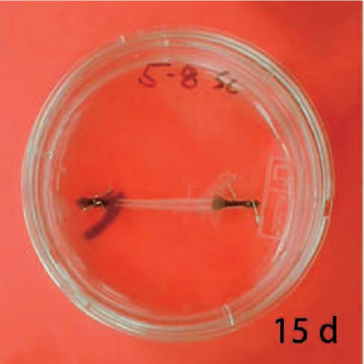
Figure 7: Engineered tendon constructs. See Calve et al. (2004) for details.

\psfrag{D}{\small$1.1284$ mm}\psfrag{H}{\small$12.0$ mm}\includegraphics[width=142.26378pt]{mesh.eps}

Figure 8: The finite element mesh used in the computations.

The theory presented in the preceding sections results in a system of non-linear, coupled partial differential equations. A finite element formulation employing a staggered scheme based upon operator splits Armero (1999); Garikipati and Rao (2001) has been implemented in FEAP (Taylor, 1999) to solve the coupled problem. As an example, in the biphasic problem involving solid and fluid phases only, the basic solution scheme involves keeping the displacement field fixed while solving for the concentration fields using the mass transport equations. The resulting concentration fields are then fixed to solve the mechanics problem. This procedure is repeated until the resulting fields satisfy the differential equations within a specified numerical tolerance.

The following examples aim to demonstrate the mathematical formulation and aspects of the coupled phenomena as the tissue grows. The model geometry, based on our engineered tendon constructs (see Figure 7 and Calve et al. (2004)), is a cylinder 12 mm in length and 1 mm² in cross-sectional area. The corresponding finite element mesh using hexahedral elements, is shown in Figure 8.

The following numerical examples involve solution of a common set of partial differential equations. The constutive models, however, vary as we demonstrate the behaviour engendered by the many modelling assumptions discussed in the paper. The balance of linear momentum that we solve is (6) summed for $\iota=\mathrm{c,f}$, with the constraint in (7) imposed. The absence of significant acceleration in the problems under consideration allows us to solve the balance of linear momentum quasi-statically. The fluid mass balance equation is solved in the current configuration, i.e. (3) for $\iota=\mathrm{f}$, but mass balance for the solid collagenous phase is solved in the reference configuration, i.e. (1) for $\iota=\mathrm{c}$. Mass balance for the solute is also solved in the current configuration, but using the stabilized scheme in weak form (23). The Backward Euler algorithm is used for all mass transport equations. The constitutive relation for the solid collagen follows (8). The constitutive relation for the fluid stress follows (9) with

$$h(\rho^{\mathrm{f}})=\frac{1}{2}\kappa^{\mathrm{f}}\left(\frac{\rho_{0_{\mathrm{ini}}}^{\mathrm{f}}}{\rho^{\mathrm{f}}}-1\right)^{2},$$ (26)

where $\kappa^{\mathrm{f}}$ is the fluid bulk modulus. The tissue is modelled as being fluid saturated in $\Omega_{t}$ at $t=0$, i.e. (5₁) holds with $\rho^{\mathrm{f}}_{0_{\mathrm{sat}}}=\rho^{\mathrm{f}}_{0_{\mathrm{ini}}}$. However, the tissue is allowed to become unsaturated in $\Omega_{t}$ for $t>0$ due to void formation. Then, the conditions set out in (11) apply. The chemical potential is then given by (13). The numerical examples that follow discuss further specialization of the constitutive relations to other cases discussed in the preceding sections. The numerical values of parameters that have been used appear in Table 1.

Non-linear projection methods (Simo et al., 1985) are used to treat the near-incompressibility imposed by the fluid. Mixed methods, as described in Garikipati and Rao (2001), are used for stress (and strain) gradient driven fluxes.

The initial and boundary conditions have been chosen in order to model a few common mechanical and chemical interventions on engineered tissue. However, we will not attempt detailed descriptions of experiments, choosing to focus instead on results that can be directly related to the models. A more detailed comparison with experiments is forthcoming in a separate communication.

4.1 A multiphasic problem based on enzyme-kinetics

Parameter (Symbol)	Value	Units
Chain density ($N$)	$7\times 10^{21}$	$\mathrm{m}^{-3}$
Temperature ($\theta$)	$310.6$	K
Persistence length ($A$)	$2.10$	–
Fully-stretched length ($L$)	$2.125$	–
Unit cell axes ($a,\;b,\;c$)	$1.95,\;1.95,\;2.43$	–
Bulk compressibility factors ($\gamma,\;\beta$)	$1000,\;4.5$	–
Fluid bulk modulus ($\kappa^{f}$)	$1$	GPa
Fluid mobility tensor ($D^{\mathrm{f}}_{ij}=D^{\mathrm{f}}\delta_{ij}$)	$1\times 10^{-14}$	s
Fibroblast concentration ($\rho_{\mathrm{cell}}$)	0.2	kg.m-3
Max. reaction rate ($k_{\mathrm{max}}=5$)	5	s-1
Max. solute concentration ($\rho^{\mathrm{s}}_{m}$)	0.2	kg.m-3
Solute diffusivity ($\mbox{\boldmath$D$}^{\mathrm{s}}$)	$1\times 10^{-9}$	m-2s

Table 1: Material parameters used in the analysis.

This first example can be viewed as a model for localised, bolus delivery of regulatory chemicals to the tendon while accounting for mechanical (stress) effects. A single solute species is considered, denoted by s, and a uniform distribution of fibroblasts that are characterised by their cell concentration, $\rho_{\mathrm{cell}}$. Both, Fickean diffusion of the solute, and stress gradient driven fluid flow are incorporated in this illustration. We use Michaelis-Menten enzyme kinetics [Equation (24)] to determine the rates of solute consumption and collagen production as a function of solute concentration. This non-linear relationship for our choice of parameters is visualised in Figure 9. Here, the fluid phase does not take part in reactions, and hence $\Pi^{\mathrm{f}}=0$.

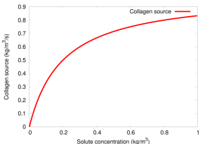
Figure 9: Variation of the collagen source term (kg.m^-3.s^-1) with solute concentration (kg.m^-3).

The tendon immersed in the bath is subjected to a constrictive radial load, such as would be imposed upon manipulating it with a set of tweezers, as depicted in Figure 10. The maximum strain in the radial direction—experienced half-way through the height of the tendon—is 10%. The applied strain in the radial direction decreases linearly with distance from the central plane, and vanishes at the top and bottom surfaces of the tendon.

\psfrag{M}{\small$\mbox{\boldmath$N$}\cdot\mbox{\boldmath$M$}^{f}$}\psfrag{P}{\small${\tiny\quad}\leavevmode\nobreak\ \mbox{\boldmath$u$}$}\includegraphics[width=142.26378pt]{cylinder-in-bath.eps}

Figure 10: Constrictive load applied to tendon immersed in a bath.

The initial collagen concentration and the initial fluid concentration are both 500 kg.m^-3 at every point in the tendon, and the fluid concentration in the bath is 500 kg.m^-3. In addition, a solute-rich bulb of radius 0.15 mm is introduced with its centre on the axis of the tendon and situated 3 mm below the upper circular face of the tendon. The initial solute concentration is 0.05 kg.m^-3 at all other points in the tendon, and increases linearly with decreasing radius in this bulb to 1 kg.m^-3 at its centre (see Figure 11). The parameters used are listed in Table 1, and are relevant to tendons.

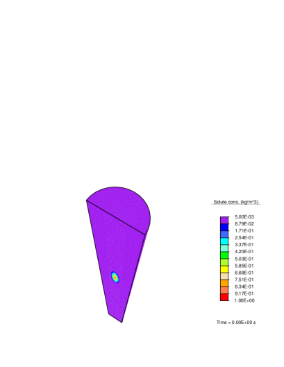
Figure 11: The solute concentration (kg.m^-3) initially.

The aim of this example is to compare the influences upon solute transport from two mechanisms: Fluid stress gradient-driven transport, arising from the applied constrictive load, and solute concentration gradient-driven transport. These mechanisms have both been implicated in nutrient supply to cells in soft tissue. The results of this numerical example demonstrate that because the magnitude of the fluid mobility for stress gradient driven transport is orders of magnitude smaller than the diffusion coefficient for the solute through the fluid, there is relatively only a small stress gradient driven flux, and the transport of the solute is diffusion dominated. As a result, the solute diffuses locally, but displays no observable advection along the fluid. As the diffusion-driven solute concentration in a region increases, the enzyme-kinetics model results in a small source term for collagen production, and we observe nominal growth. Figure 12 shows the collagen concentration at an early time, $t=5\times 10^{-2}$ s.

Figure 12: The collagen concentration (kg.m^-3) at time $t=5\times 10^{-2}$ s.

This example incorporates all of the theory discussed in the paper. However, it is a valuable exercise in modelling to simplify the boundary value problem, and supress some of the coupled phenomena in order to gain a better understanding of some effcts. This is the approach followed in the next two numerical examples. The detailed transport and mechanics induced by the constrictive radial load are discussed first in Section 4.2.1.

4.2 Examples exploring the biphasic nature of porous soft tissue

In these calculations, only two phases—fluid and collagen—are included for the mass transport and mechanics. The parameters used in the analysis are presented in Table 1.

4.2.1 The tendon under constriction

In this example, the tendon immersed in a bath is subjected to the same constrictive radial load as in Section 4.1. Since that example demonstrated an insignificant amount of local collagen production over this time scale, we have simplified the problem by setting the source term $\Pi^{\mathrm{c}}=0$. The total duration of the simulation is 10 s, and the radial strain is applied as a displacement boundary condition, increasing linearly from no strain initially to the maximum strain at time $t=1\leavevmode\nobreak\ \mathrm{s}$. Again, both the initial collagen concentration and the initial fluid concentration are 500 kg.m^-3 at every point in the tendon. This tendon is exposed to a bath where the fluid concentration is 500 kg.m^-3.

While solving the balance of momentum for the biphasic problem of the solid collagen and a fluid phase, we currently treat the tissue as a single entity and employ a summation of Equation (6) over both species. Additionally, condition (7) allows us to avoid constitutive prescription of the momentum transfer terms between solid collagen and fluid phases, $\mbox{\boldmath$q$}^{\mathrm{c}}$ and $\mbox{\boldmath$q$}^{\mathrm{f}}$. This facilitates considerable simplification of the problem, but such a treatment requires additional assumptions on the detailed deformation of the constitutive phases of the tissue. An explicit assumption we have drawn on thus far is the equality of the deformation gradient of the solid collagen and pore spaces, allowing us to use the deformation gradient $F$, suitably decomposed to account for change in fluid concentration, to model the fluid stress. This assumption and its consequences have been discussed in Sections 2.1, 2.2, 2.2.1, 3.2, 3.2.1 and 3.3.4. Since the imposition of a common deformation gradient results in an upper bound for the effective stiffness of the tissue and magnitudes of the fluxes established, we refer to it as the upper bound model. This assumption plays a fundamental role in determining the fluid flux driven by the fluid stress gradient.

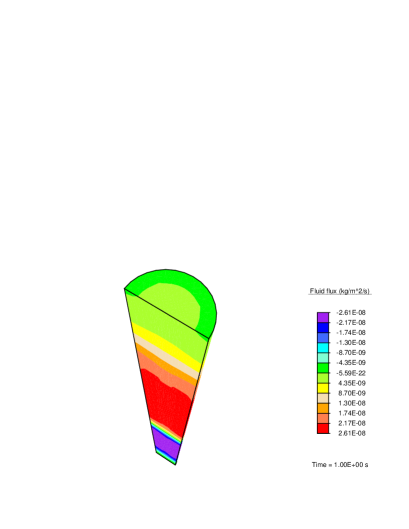
Figure 13: Upper bound fluid flux (kg.m^-2.s^-1) in the vertical direction at time $t=1$ s.

For this upper bound model, Figure 13 shows the fluid flux in the vertical direction at the final stage of the constriction phase of the simulation, i.e. at time $t=1$ s. The flux values are positive above the central plane, forcing fluid upward, and negative below, forcing fluid fluid downward. This stress-gradient induced fluid flux results in a reference concentration distribution of the fluid that is higher near the top and bottom faces, as seen in Figure 14.

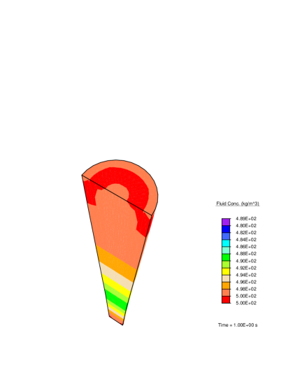
Figure 14: Reference fluid concentration (kg.m^-3) at time $t=1$ s.

As a result, these regions would have seen a higher production of collagen, or preferential growth, in the presence of non-zero source terms. As discussed in Section 2.1.1, the mass transport equations are solved in the current configuration, where physical boundary conditions can be set directly. The values reported in Figure 14 are pulled back from the current configuration. The current concentrations do not change for this boundary value problem.

Solving a problem of this nature in the reference configuration using $\rho_{0}^{\mathrm{f}}=$ const. as the boundary condition to represent immersion of the tendon in a fluid bath yields non-physical results, such as an unbounded flow. This occurs since the imposed strain gradient causes a stress gradient in the fluid that does not decay. The imposed boundary condition on $\rho_{0}^{\mathrm{f}}$ prevents a redistribution of concentration that would have provided an opposing, internal gradient of stress, which in turn would drive the flux to vanish.

The tendon is held fixed in the radial direction after the constriction phase. The applied stress sets up a pressure wave in the fluid travelling toward the top and bottom faces. As the fluid leaves these surfaces, we observe that the tendon relaxes. This is seen in Figure 15, which plots the vertical displacement of the top face with time, showing a decrease in height of the tendon after the constriction phase. We keep the centre of the bottom face of the tendon fixed.

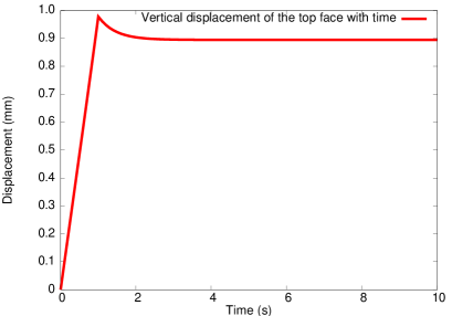
Figure 15: Relaxation of the top face of the tendon after the constriction phase.

In order to define a range of the magnitude of fluid flux, we now introduce the lower bound model (on effective stiffness of the tissue and, consequently, the magnitude of the fluid flux). For this lower bound, we replace the earlier strain homogenisation requirement with a stress homogenisation requirement, viz. equating the hydrostatic stress of the solid phase and the fluid pressure in the current configuration:

$$p^{\mathrm{f}}=\frac{1}{3}\mathrm{\small{tr}}[\mbox{\boldmath$\sigma$}^{c}],$$ (27)

where $p^{\mathrm{f}}$ is the fluid pressure in the current configuration, tr[•] is the trace operator, and $\mbox{\boldmath$\sigma$}^{c}=\frac{1}{\mathrm{J^{c}}}\mbox{\boldmath$P$}^{\mathrm{c}}\mbox{\boldmath$F$}^{\mathrm{c}^{\mathrm{T}}}$ is the Cauchy stress of the solid. The Cauchy stress of an ideal fluid can be defined from its current pressure as $\mbox{\boldmath$\sigma$}^{f}=p^{\mathrm{f}}{\bf 1}$. Figure 16 reports the value of the vertical flux under the lower bound modelling assumption, using boundary conditions identical to the previous calculation at time $t=1$ s, the final stage of the constriction phase of the simulation.

Figure 16: Lower bound fluid flux (kg.m^-2.s^-1) in the vertical direction at time $t=1$ s.

The fluid flux values reported in Figures 13 and 16 (corresponding to the upper and lower bound modelling assumptions, respectively) are qualitatively similar, but differ by about three orders of magnitude. This wide range points to the importance of imposing the appropriate mechanical coupling model between interacting phases. Note, however, that we have computed bounds for the range of possible fluid flux values under the specified mechanical loading. Recall, furthermore, that the example in Section 4.1 used the upper bound model, and yet resulted in no discernible advective solute transport. This suggests strongly that, given the parameters in Table 1, convective transport of nutrients in tendons is dominated by diffusive transport. In future work, we will detail models that result in precise field values for the fluxes, which will replace the upper and lower bounds discussed here.

This numerical example also points to the fact that a convenient measure of the strength of coupling between the mechanics and mass transport equations is the ratio of the variation in hydrostatic stress of the fluid to that of the solid. In the lower bound case, where the fluid response is defined by Equation (27), it is instructive to note that this ratio is unity. As a result, it is seen that the lower bound case exhibits significantly weaker coupling than the upper bound case. In the latter, variation in the common deformation gradient, $\delta\mbox{\boldmath$F$}$, causes instantaneous variation in $\delta p^{\mathrm{f}}\approx O(\kappa^{\mathrm{f}}\delta\mbox{\boldmath$F$}:\mbox{\boldmath$F$}^{-\mathrm{T}})$ and in $\frac{1}{3}\delta\mathrm{\small{tr}}[\mbox{\boldmath$\sigma$}^{c}]\approx O(\kappa^{\mathrm{c}}\delta\mbox{\boldmath$F$}:\mbox{\boldmath$F$}^{-\mathrm{T}})$, where $\kappa^{\mathrm{c}}$ is the bulk modulus of the solid. The ratio $\frac{\delta p^{\mathrm{f}}}{\frac{1}{3}\delta\mathrm{\small{tr}}[\mbox{\boldmath$\sigma$}^{c}]}$ is therefore $\approx O(\kappa^{\mathrm{f}}/\kappa^{\mathrm{c}})\gg 1$.

The strength of coupling between the equations plays a principal role in the rate of convergence of the solution, as observed in Table 2, where the residual norms of the equilibrium equation (and corresponding CPU times in seconds for an Intel®Xeon 3.4 GHz machine) are reported for the first 8 iterations of each of the two cases. Recall that the staggered scheme involves solution of the mechanics equation keeping the concentrations fixed, and the mass transport equation keeping the displacements fixed, in turn, until the solution converges. The table does not report the value of the residual norms arising from the solution of the mass transport equation for the fluid, which occurs after each reported solve of the of the mechanics equation. Although the initial mechanics residual norms in successive passes are decreasing linearly in both cases, the rapid decrease in this quantity in the weakly-coupled case ensures convergence in far fewer iterations than the strongly coupled case. Thus, the corresponding CPU times reported are also lower for the weakly coupled case. This is advantageous. In addition to being more physical, as argued at the beginning of Section 4.2.2 immediately below, the lower bound, weakly-coupled case makes it feasible to drive problems to longer, physiologically-relevant time-scales through the use of larger time steps.

Pass	Strongly coupled		Weakly coupled
	Residual	CPU (s)	Residual	CPU (s)
1	$2.138\times 10^{-02}$	29.16	$6.761\times 10^{-04}$	28.5
	$3.093\times 10^{-04}$	55.85	$1.075\times 10^{-04}$	55.1
	$2.443\times 10^{-06}$	82.37	$4.984\times 10^{-06}$	81.8
	$2.456\times 10^{-08}$	109.61	$1.698\times 10^{-08}$	107.9
	$4.697\times 10^{-14}$	135.83	$3.401\times 10^{-13}$	134.1
	$1.750\times 10^{-16}$	163.18	$1.1523\times 10^{-17}$	161.1
2	$5.308\times 10^{-06}$	166.79	$5.971\times 10^{-08}$	192.5
	$4.038\times 10^{-10}$	193.36	$4.285\times 10^{-11}$	218.6
	$1.440\times 10^{-14}$	220.45	$2.673\times 10^{-15}$	246.1
	$4.221\times 10^{-17}$	247.04
3	$5.186\times 10^{-06}$	250.62	$2.194\times 10^{-09}$	277.3
	$3.852\times 10^{-10}$	277.44	$2.196\times 10^{-13}$	304.2
	$1.369\times 10^{-14}$	304.16	$1.096\times 10^{-17}$	331.6
	$4.120\times 10^{-17}$	331.47
4	$5.065\times 10^{-06}$	335.16	$8.160\times 10^{-11}$	363.2
	$3.674\times 10^{-10}$	362.24	$7.923\times 10^{-15}$	390.2
	$1.300\times 10^{-14}$	388.79
	$4.021\times 10^{-17}$	416.08
5	$4.948\times 10^{-06}$	419.59	$3.078\times 10^{-12}$	421.4
	$3.503\times 10^{-10}$	446.24	$3.042\times 10^{-16}$	448.6
	$1.236\times 10^{-14}$	473.20
	$3.924\times 10^{-17}$	500.85
6	$4.832\times 10^{-06}$	504.65	$1.179\times 10^{-13}$	479.9
	$3.340\times 10^{-10}$	531.28	$1.291\times 10^{-17}$	507.0
	$1.174\times 10^{-14}$	558.17
	$3.829\times 10^{-17}$	585.27
7	$4.720\times 10^{-06}$	589.01	$4.592\times 10^{-15}$	537.8
	$3.184\times 10^{-10}$	616.24	$5.152\times 10^{-18}$	564.6
	$1.116\times 10^{-14}$	643.29
	$3.737\times 10^{-17}$	670.83
8	$4.609\times 10^{-06}$	674.46	$1.816\times 10^{-16}$	595.5
	$3.034\times 10^{-10}$	701.74	$5.040\times 10^{-18}$	622.3
	$1.060\times 10^{-14}$	727.74
	$3.646\times 10^{-17}$	755.58

Table 2: Mechanics equation residual norms and corresponding CPU times in seconds for the first 8 passes of each of the two cases for a typical time increment, $\Delta t=$ 0.1 s.

4.2.2 A swelling problem

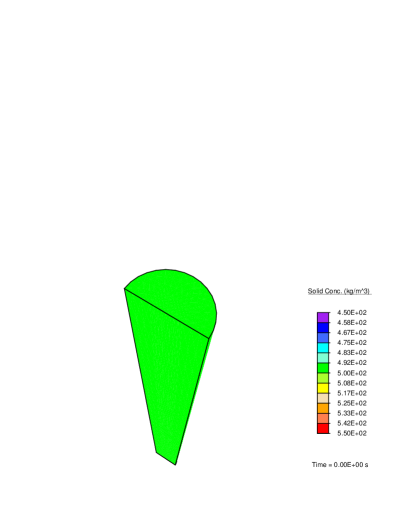
Figure 17: The collagen initial concentration (kg.m^-3).

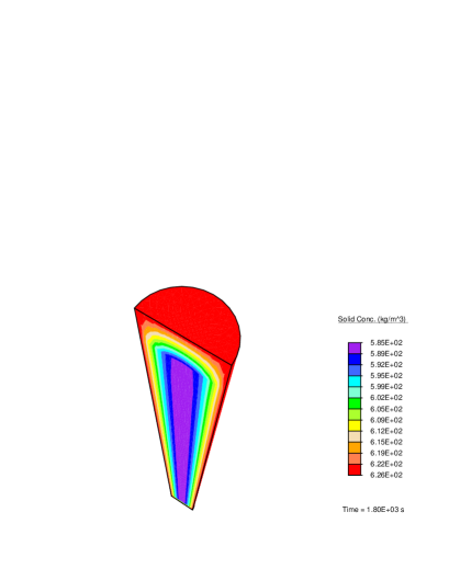
Figure 18: The collagen concentration (kg.m^-3) after 1800 s.

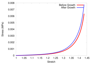
Figure 19: The stress (Pa) vs stretch curves before and after growth.

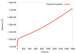
Figure 20: The volume of the tendon (m³) evolving with time. Note the fluid transported-dominated regime until 25 s, followed by the longer reaction-dominated growth stage.

Motivated mainly by the recognition that the lower bound model for solid-fluid mechanical coupling ensures convergence to a self-consistent solution in just a few passes of the staggered solution scheme, we adopt this version of the coupling for our final problem. On this note we point out that solution of the individual balances of linear momentum equation for the solid collagenous and fluid phases with the momentum transfer terms [$\mbox{\boldmath$q$}^{\mathrm{c}},\mbox{\boldmath$q$}^{\mathrm{f}}$ in (6)] is a statement of momentum balance between them. There is reason to suppose, therefore, that equating the solid collagen and fluid stress, or some component of these tensors as done in the lower bound model, is a reasonable approximation to explicitly solving the balance of linear momentum for each phase, including the momentum transfers. In contrast, equating the deformation gradient of the solid collagen with deformation of the pore spaces subjects the fluid to a stress state also determined by this deformation gradient in the upper bound model. This approximation does not correspond to an underlying physical principle comparable to the satisfaction of individual balances of linear momentum for solid collagen and fluid, with momentum transfers. It is therefore somewhat less motivated and more questionable. Clearly, a rigorous analysis or numerical comparisons of all three models: upper bound, lower bound and direct solution of individual solid-fluid momentum balances, must be carried out to conclusively demonstrate this. It is a possible topic for a future paper.

In this example we will demonstrate the mechanical effects of growth due to collagen production. In the interest of focusing on this issue we assume that fibroblasts are available, and that the fluid phase bears the necessary nutrients for collagen production dissolved at a suitable, constant concentration. Collagen production is assumed to be governed by a first-order rate law. Newly-produced collagen has proteoglycan molecules bound to it, and they in turn bind water. We model this effect by associating a loss of nutrient-bearing free fluid with collagen production. A fluid sink $\Pi^{\mathrm{f}}$ is introduced following first order kinetics,

$$\Pi^{\mathrm{f}}=-k^{\mathrm{f}}(\rho_{0}^{\mathrm{f}}-\rho_{0_{\mathrm{ini}}}^{\mathrm{f}}),$$ (28)

as in Garikipati et al. (2004). Here $k^{\mathrm{f}}$ is the reaction rate, taken to be 0.07 $\mathrm{s}^{-1}$, and $\rho_{0_{\mathrm{ini}}}^{\mathrm{f}}$ is the initial concentration of fluid. The collagen source is mathemaically equivalent to the fluid sink: $\Pi^{\mathrm{c}}=-\Pi^{\mathrm{f}}$. When $\rho_{0}^{\mathrm{f}}>\rho_{0_{\mathrm{ini}}}^{\mathrm{f}}$, collagen is produced.

The boundary conditions in this example correspond to immersion of the tendon in a nutrient-rich bath. The initial collagen concentration is 500 kg.m^-3 and the fluid concentration is 400 kg.m^-3 at every point in the tendon. When this tendon is exposed to a bath where the fluid concentration is 410 kg.m^-3, i.e. $\rho^{\mathrm{f}}(\mbox{\boldmath$x$},t)=410\leavevmode\nobreak\ \mathrm{kg.m}^{-3}\forall\mbox{\boldmath$x$}\in\partial\Omega_{t}$, nutrient-rich fluid is transported into the tissue, due to the pressure difference, induced by the concentration difference, between the fluid in the tendon and in the bath (fluid stress gradient-driven flux). Thereby, the nutrient concentration is elevated, leading to collagen production, fluid consumption and, eventually, growth due to additional collagen.

Figure 17 shows the initial collagen concentration in the tendon. After it has been immersed in the nutrient-rich bath for 1800 s, the tendon shows growth and the collagen concentration is higher as seen in Figure 18. On performing a uniaxial tension test on the tendon before and after growth, it is observed (Figure 19) that the grown tissue is stiffer and stronger due to its higher collagen concentration. Also note that there is a rapid, fluid transport-dominated swelling of the tendon between 0 and 25 s following immersion in the fluid bath (Figure 20). This causes a small volume change of $\approx 1.6$%. In this transport-dominated regime the contribution to tendon growth from collagen production is small. However, the fluid-induced swelling saturates, and between 25 and 1800 s the reaction producing collagen dominates the growth process, producing a further $\approx 6.8$% volume change. Noting that the range of collagen concentration in Figure 18 is $585-626\;\mbox{kg.m}^{-3}$, and that (4) gives $\mbox{\boldmath$F$}^{\mathrm{g}^{\mathrm{c}}}=\left(\frac{\rho_{0}^{\mathrm{c}}}{\rho_{0_{\mathrm{ini}}}^{\mathrm{c}}}\right)^{\frac{1}{3}}{\bf 1}$, this portion of the volume change is quite clearly due to collagen production. The total volume change of $8.4$% corresponds to changes in each linear dimension of the tendon by only $\approx 2.7$%, and is not discernible upon comparing Figures 17 and 18. It is, however, manifest in Figure 20.

5 Conclusion

In this paper, we have discussed a number of enhancements to our original growth formulation presented in Garikipati et al. (2004). That formulation has served as a platform for posing a very wide range of questions on the biophysics of growth. Some issues, such as saturation, incompressibility of the fluid species and its influence upon the tissue response, and the roles of biochemical and strain energy-dependent source terms are specific to soft biological tissues. We note, however, that other issues are also applicable to a number of systems with a porous solid, transported fluid and reacting solutes. Included in these are issues of current versus reference configurations for mass transport, swelling, Fickean diffusion, fluid response in compression and tension, cavitation and the strength of solid-fluid coupling..

These issues have been resolved using arguments posed easily in the framework derived in Garikipati et al. (2004). The interactions engendered in the coupled reaction-transport-mechanics system are complex, as borne out by the numerical examples in Section 4. We are currently examining combinations of sources defined in Section 3.4, and aim to calibrate our choices from tendon growth experiments. The treatment of these issues has led to a formulation more suited to the biophysics of growing soft tissue, making progress toward our broader goal of applying it to the study of wound healing, pathological hypertrophy and atrophy, as well as a study of drug efficacy and interaction.

References

- Alberts et al. (2002) Alberts B, Johnson A, Lewis J, Raff M, Roberts K, Walter P (2002) Molecular Biology of the Cell. Garland Science, Oxford
- Ambrosi and Mollica (2002) Ambrosi D, Mollica F (2002) On the mechanics of a growing tumor. Int J Engr Sci 40:1297–1316
- Armero (1999) Armero F (1999) Formulation and finite element implementation of a multiplicative model of coupled poro-pplasticity at finite strains under fully-saturated conditions. Comp Methods in Applied Mech Engrg 171:205–241
- Bischoff et al. (2002a) Bischoff JE, Arruda EM, Grosh K (2002a) A microstructurally based orthotropic hyperelastic constitutive law. J Applied Mechanics 69:570–579
- Bischoff et al. (2002b) Bischoff JE, Arruda EM, Grosh K (2002b) Orthotropic elasticity in terms of an arbitrary molecular chain model. J Applied Mechanics 69:198–201
- Brennen (1995) Brennen CE (1995) Cavitation and Bubble Dynamics. Oxford University Press
- Breward et al. (2003) Breward CJW, Byrne HM, Lewis CE (2003) A multiphase model describing vascular tumour growth. Bull Math Biol 65:609–640
- Bromberg and Dill (2002) Bromberg S, Dill KA (2002) Molecular Driving Forces: Statistical Thermodynamics in Chemistry and Biology. Garland
- Brooks and Hughes (1982) Brooks A, Hughes T (1982) Streamline upwind/Petrov-Galerkin formulations for convection dominated flows with particular emphasis on the incompressible Navier-Stokes equations. Comp Methods in Applied Mech Engrg 32:199–259
- Bustamante et al. (2003) Bustamante C, Bryant Z, Smith SB (2003) Ten years of tension: Single-molecule DNA mechanics. Nature 421:423–427
- Calve et al. (2004) Calve S, Dennis R, Kosnik P, Baar K, Grosh K, Arruda E (2004) Engineering of functional tendon. Tissue Engineering 10:755–761
- Cowin and Hegedus (1976) Cowin SC, Hegedus DH (1976) Bone remodeling I: A theory of adaptive elasticity. Journal of Elasticity 6:313–325
- Epstein and Maugin (2000) Epstein M, Maugin GA (2000) Thermomechanics of volumetric growth in uniform bodies. International Journal of Plasticity 16:951–978
- Fung (1993) Fung YC (1993) Biomechanics: Mechanical properties of living tissues, 2nd edn. Springer-Verlag, New York
- Garikipati and Rao (2001) Garikipati K, Rao VS (2001) Recent advances in models for thermal oxidation of silicon. Journal of Computational Physics 174:138–170
- Garikipati et al. (2001) Garikipati K, Bassman LC, Deal MD (2001) A lattice-based micromechanical continuum formulation for stress-driven mass transport in polycrystalline solids. Journal of Mechanics and Physics of Solids 49:1209–1237
- Garikipati et al. (2004) Garikipati K, Arruda EM, Grosh K, Narayanan H, Calve S (2004) A continuum treatment of growth in biological tissue: Mass transport coupled with mechanics. Journal of Mechanics and Physics of Solids 52:1595–1625
- Han et al. (2000) Han S, Gemmell SJ, Helmer KG, Grigg P, Wellen JW, Hoffman AH, Sotak CH (2000) Changes in ADC caused by tensile loading of rabbit achilles tendon: Evidence for water transport. Journal of Magnetic Resonance 144:217–227
- Harrigan and Hamilton (1993) Harrigan TP, Hamilton JJ (1993) Finite element simulation of adaptive bone remodelling: A stability criterion and a time stepping method. Int J Numer Methods Engrg 36:837–854
- Hughes et al. (1987) Hughes T, Franca L, Mallet M (1987) A new finite element formulation for computational fluid dynamics: VII. Convergence analysis of the generalized SUPG formulation for linear time-dependent multidimensional advective-diffusive systems. Comp Methods in Applied Mech Engrg 63(1):97–112
- Humphrey and Rajagopal (2002) Humphrey JD, Rajagopal (2002) A constrained mixture model for growth and remodeling of soft tissues. Math Meth Mod App Sci 12(3):407–430
- Klisch and Hoger (2003) Klisch SM, Hoger A (2003) Volumetric growth of thermoelastic materials and mixtures. Math Mech Solids 8:377–402
- Klisch et al. (2001) Klisch SM, van Dyke TJ, Hoger A (2001) A theory of volumetric growth for compressible elastic biological materials. Math Mech Solids 6:551–575
- Kratky and Porod (1949) Kratky O, Porod G (1949) Röntgenuntersuchungen gelöster Fadenmoleküle. Recueil Trav Chim 68:1106–1122
- Kuhl and Steinmann (2003) Kuhl E, Steinmann P (2003) Theory and numerics of geometrically-nonlinear open system mechanics. Int J Numer Methods Engrg 58:1593–1615
- Kuhl et al. (2005) Kuhl E, Garikipati K, Arruda E, Grosh K (2005) Remodeling of biological tissue: Mechanically induced reorientation of a transversely isotropic chain network. J Mech Phys Solids (UK) 53(7):1552 – 73
- Landau and Lifshitz (1951) Landau LD, Lifshitz EM (1951) A Course on Theoretical Physics, Volume 5, Statistical Physics, Part I. Butterworth Heinemann (reprint)
- Lee (1969) Lee EH (1969) Elastic-Plastic Deformation at Finite Strains. J Applied Mechanics 36:1–6
- Marko and Siggia (1995) Marko JF, Siggia ED (1995) Stretching DNA. Macromolecules 28:8759–8770
- Nordin et al. (2001) Nordin M, Lorenz T, Campello M (2001) Biomechanics of tendons and ligaments. In: Nordin M, Frankel VH (eds) Basic Biomechanics of the Musculoskeletal System, Lippincott Williams and Wilkins, N.Y., pp 102–125
- Preziosi and Farina (2002) Preziosi L, Farina A (2002) On Darcy’s Law for growing porous media. Int J Non-linear Mech 37:485–491
- Provenzano et al. (2003) Provenzano PP, Martinez DA, Grindeland RE, Dwyver KW, Turner J, Vailas AC, Vanderby R (2003) Hindlimb unloading alters ligament healing. Journal of Applied Physiology 94:314–324
- Rao et al. (2000) Rao VS, Hughes TJR, Garikipati K (2000) On modelling thermal oxidation of silicon ii: Numerical aspects. ijnme 47(1/3):359–378
- Rief et al. (1997) Rief M, Oesterhelt F, Heymann B, Gaub HE (1997) Single Molecule Force Spectroscopy of Polysaccharides by Atomic Force Microscopy. Science 275:1295–1297
- Sengers et al. (2004) Sengers BG, Oomens CWJ, Baaijens FPT (2004) An integrated finite-element approach to mechanics, transport and biosynthesis in tissue engineering. J Bio Mech Engrg 126:82–91
- Simo et al. (1985) Simo JC, Taylor RL, Pister KS (1985) Variational and projection methods for the volume constraint in finite deformation elasto-plasticity. Comp Methods in Applied Mech Engrg 51:177–208
- Sun et al. (2002) Sun YL, Luo ZP, Fertala A, An KN (2002) Direct quantification of the flexibility of type I collagen monomer. Biochemical and Biophysical Research Communications 295:382–386
- Swartz et al. (1999) Swartz M, Kaipainen A, Netti PE, Brekken C, Boucher Y, Grodzinsky AJ, Jain RK (1999) Mechanics of interstitial-lymphatic fluid transport: Theoretical foundation and experimental validation. J Bio Mech 32:1297–1307
- Taber and Humphrey (2001) Taber LA, Humphrey JD (2001) Stress-modulated growth, residual stress and vascular heterogeneity. J Bio Mech Engrg 123:528–535
- Taylor (1999) Taylor RL (1999) FEAP - A Finite Element Analysis Program. University of California at Berkeley, Berkeley, CA
- Tezduyar and Sathe (2003) Tezduyar T, Sathe S (2003) Stabilization parameters in SUPG and PSPG formulations. Journal of Computational and Applied Mechanics 4:71–88
- Truesdell and Noll (1965) Truesdell C, Noll W (1965) The Non-linear Field Theories (Handbuch der Physik, band III). Springer, Berlin