Microcolony and Biofilm Formation
as a Survival Strategy for Bacteria

Abstract

Bacterial communities such as biofilms are widely recognised as being important for survival and persistence of bacteria in harsh environments. Mechanistic models of biofilm growth indicate that the way in which the surface is seeded can effect the morphology of simulated biofilms. Experimental studies indicate that genes which are important for chemotaxis also influence biofilm formation, perhaps by influencing aggregation on a surface. Understanding aggregation and microcolony formation could therefore help clarify factors influencing biofilm formation as well as understanding how groups may influence the fitness of bacteria. In this paper I develop an Individual Based Model to examine how different behaviours involved in microcolony formation on a surface determine patterns of group sizes, and link patterns to bacterial fitness. I also provide a method for comparing data with model hypotheses to identify bacterial behaviours in experimental systems.

Keywords: biofilm; Individual based model; bacterial fitness

1 Introduction

Bacteria live in communities for many of the same reasons that other organisms live in communities; for example protection from predators or other external dangers and access to resources, and genetic diversity [Jefferson, 2004, Roszak and Colwell, 1987]. Individuals in many bacterial communities, such as in biofilms, experience increased resistance to antibiotics, thermal stress, or predation [Hahn and Höfle, 2001, Matz et al., 2005]. These communities also allow bacteria to stay in favourable environments without being swept away. Bacterial fitness depends strongly on how quickly the cells can double. However, because doubling rates of individuals in a community are generally lower than doubling rates of individuals outside of communities, living in a community often represents a trade-off between reproduction and survival.

Community types and morphologies are determined by physical, biochemical, and genetic factors. Physical and biochemical factors – such as fluid flow, polymer tensile strength, and cell surface properties – influence the availability of nutrients within a community, the ability of a biofilm to hold together under shear stress, and determine whether or not cells can stick to a particular surface. Genetic factors constrain the behavioural options available to the bacteria, and determine responses to chemical or environmental signals. Current research indicates that gene expression of bacteria living in biofilms or other communities differs significantly from that of free-living cells, and may be mediated by a process called quorum sensing [Davies et al., 1998, Heydorn et al., 2002, Parsek and Greenberg, 2005].

Genes that regulate the production of extra-cellular polymeric substances (EPS) are widely recognised as influencing biofilm formation [Branda et al., 2005, Davey and O’Toole, 2000, Mayer et al., 1999, Yildiz and Schoolnik, 1999, Watnick and Kolter, 1999]. Current research indicates that genes involved in flagellar motility and various chemotaxis and quorum sensing systems also appear to also influence the ability of many types of bacteria, for instance toxigenic Vibrio cholerae, to form biofilms, as well as influencing the morphology of the biofilms [Davies et al., 1998, Heydorn et al., 2002, Parsek and Greenberg, 2005, Suntharalingam and Cvitkovitch, 2005]. Since many bacteria in biofilms appear to down-regulate motility genes, it has been hypothesised that aggregation of bacteria on a surface is an important step in the development of biofilms [Watnick and Kolter, 1999]. However, data on the role of aggregation in initial stages of microcolony formation are inconclusive [Klausen et al., 2003]. This is partly due to the fact that bacterial aggregation is difficult to observe directly. Observations of densities are influenced by both aggregation and reproduction. It can also be very difficult to monitor individual bacteria on a surface, since many microscopic techniques that are able to clearly discern individual cells, such as confocal or scanning electron microscopy, often damage or kill cells.

Since aggregation can be hard to observe directly, mathematical models that can predict observable macroscopic patterns indicative of aggregation are desirable. Models also allow exploration of how bacterial behaviours change macroscopic patterns, and help in linking these behaviours to the function of various genes.

In this paper I introduce an Individual Based Model (IBM) for microcolony formation on a surface. I seek to addresses three major questions. First, how do interactions between cells and cell behaviours influence microcolony characteristics such as size? Second, can we differentiate between different kinds of behaviours from “snapshots” of growing microcolonies? Finally, how might these behaviours and the resulting patterns be linked to bacterial fitness?

2 Approaches for Modelling Bacterial Communities

Models of communities of micro-organisms, as well as larger organisms, generally take one of three approaches. The first approach to is generally referred to as Eulerian methods. These are continuous models, focused on developing field equations that describe the flux of individuals in space. This type of approach ignores individual identity, instead focusing on densities of individuals in an area or volume. Examples of this approach include Keller and Segel’s models of slime mold aggregation [Keller and Segel, 1970] and bacterial chemotaxis [Keller and Segel, 1971a, Keller and Segel, 1971b], models of midge swarming [Tyutyunov et al., 2004], and a general approach to group formation in animals proposed by Gueron and Levin [Gueron and Levin, 1995]. The Eulerian approach is most useful for describing very large numbers of individuals with high density. It also has an advantage that there are many good analytical tools available. However, if the density of individuals is low, or one wishes to explore how individual strategies effect group dynamics, this type of approach is less useful [Gueron et al., 1996].

A second approach uses Cellular Automata (CA) [Wolfram, 2002]. CA are a class of discrete dynamical models where the space occupied is divided into grids or boxes (often called cells, but for our purpose here they will be referred to as elements) on a lattice. Each element is characterised by some description of the element’s state at some time $t$, which is often discrete. The state of each element can be updated by a set of rules that may depend on the current state of the element as well as the states of neighbour elements. This method is especially popular for modelling biofilm formation. For models of biofilms, the state of each element contains information about whether the cell is occupied by biomass of particular density and type. Such models are sometimes referred to as biomass-based models (BbM) [Kreft et al., 2001].

Some of the most detailed biofilm models, developed by Picioreanu et al. [Picioreanu et al., 1998, Picioreanu et al., 1999, Picioreanu and van Loosdrecht, 2003, van Loosdrecht et al., 2002], involve a CA model for the spreading of biomass, including living and dead cells and extra-cellular polymeric substances (EPS). Additionally, these methods include substrate transport via diffusion and convection, and can include modelling of detachment due to mechanical stress from fluid flow over the biofilm.

Although both Eulerian and CA models can provide information about macroscopic properties of systems, they ignore both variation of traits between individuals and interactions between individuals. Since both of these can greatly effect the dynamics of the larger system that the individuals compose, a third approach, Individual Based Models (IBMs) [Grimm and Railsback, 2005] can be used to explore these phenomena explicitly. IBMs comprise models where the behaviour of each individual is modelled separately, and each individual follows a set of rules that determine their behaviour.

IBM models are variants of $N$-body Newtonian dynamics problems, and are often called Lagrangian models. The rules that control individuals are a combination of forces and decision rules. Examples of forces include those that are physical or environmental (such as chemical gradients, gravity, or drag), and other such as attraction or repulsion between individuals [Okubo, 1986, Gueron et al., 1996]. Regardless of the types of decisions or forces chosen, the goal is to learn about how interactions and behaviours on small scales influence large-scale patterns. Additionally, once behaviours that result in “realistic” patterns have been identified, these can be compared to behaviours in populations, and used to evaluate which rules could be selected for in different situations.

BacSim [Kreft et al., 1998, Kreft et al., 2001], a model of E. coli colony growth, is an example of an IBM model of biofilm growth. It features an IBM for the growth and behaviour of individual bacteria (including uptake of substrate, death, and reproduction) together with a simulation of the diffusion and reaction of substrate and other products. BacSim simulates spreading of the biomass by requiring that a minimum distance is maintained between cells. One of the primary results of the study by Kreft et al. [Kreft et al., 2001] is that the initial seeding of a surface has a major impact on the development and morphology of simulated biofilms, especially those composed of multiple types of bacteria. This is likely because of the heterogeneity of substrate concentration in the biofilm. They concluded that “this stresses the primary importance of spreading and chance in the emergence of the complexity of the biofilm community.”

Biofilm formation is generally thought to proceed as follows:

1. individuals colonise surface

2. individuals form microcolonies

3. microcolonies form biofilms

Most current models of biofilms, regardless of approach, focus on growth of biofilms from a randomly seeded surface, using physical and chemical factors, i.e., they focus on the third step listed above. These models ignore the initial surface colonisation events and microcolony formation. They also largely ignore biochemical interactions, such as quorum sensing.

My goal is to develop an IBM that can be used with experimental data to infer the bacterial behaviours that generate the patterns observed during the initial stages of biofilm formation. I am most interested in how interactions among individuals affect microcolony sizes during initial stages of biofilm formation, and the implications the behaviours have for bacterial fitness‘. I assume that the environment is homogeneous and external forces (such as drag) are minimal. I also assume that the density of organisms is sufficiently low so that growth and reproduction are not affected by diffusion limitation, and competition for nutrients is minimal.

3 An IBM for Bacterial Community Formation

3.1 Cell State

The IBM begins with a description of the variables necessary to describe an individual cell’s state. At time $t$ a cell is characterised by a set of state variables. These variables can include the cell’s position, velocity, genotype, age, size, etc. I will denote the vector that describes the overall state of the $i^{th}$ cell as $\mathbf{S}_{i}(t)$. For the models presented here, the state of the cell is described by a combination of the variables listed in Table 1.

Symbol	Description
$\mathbf{X}_{i}$	cell position (centre of cell)
$\mathbf{F}_{i}$	force on cell
$\mathbf{V}_{i}$	velocity of cell
$\tau_{i}$	time since last division
$T_{i}$	doubling time of cell
$a_{i}$	cellular age, in number of divisions
$\gamma_{i}$	cell is moving $\gamma_{i}=1$, or stopped $\gamma_{i}=0$
$\alpha_{i}$	cell is alive $\alpha_{i}=1$, or dead $\alpha_{i}=0$
$\phi_{i}$	cell overlaps other cells $\phi_{i}=0$, otherwise $\phi_{i}=1$
$r_{i}$	cell radius
$C_{i}$	colony membership of the cell

Table 1: State Variables for the $i^{th}$ cell, included in models explored in this chapter.

I denote the stage-state of the $i^{th}$cell at time $t$ by $s_{i,t}=\{a,\gamma,\alpha,\phi\}_{i,t}$. The value of the stage-state is the component of the full state of the cell, $\mathbf{S}_{i}(t)$, that describes whether the cell is moving and whether it is alive. The cell can then transition between various stage-states, and the full states, at any time step. Figure 1 shows a graphical representation of the conditional transitions between the various stages and their probabilities, assuming the transitions are age independent. In a small increment of time from $t$ to $t+\Delta t$, a moving cell stops with probability $p_{1}$. A moving cell can also die (and thus simultaneously stop) with probability $p_{2}$. A stopped cell can die with probability $p_{3}$. Finally, a stopped but alive cell can move again with probability $p_{4}$. In other words:

$$Pr\{\gamma_{i,t+\Delta t}=0,\alpha_{i,t+\Delta t}=1\;|\;\gamma_{i,t}=1,\alpha_{i,t}=1\} =p_{1}$$

$$Pr\{\gamma_{i,t+\Delta t}=0,\alpha_{i,t+\Delta t}=0\;|\;\gamma_{i,t}=1,\alpha_{i,t}=1\} =p_{2}$$

$$Pr\{\gamma_{i,t+\Delta t}=0,\alpha_{i,t+\Delta t}=0\;|\;\gamma_{i,t}=0,\alpha_{i,t}=1\} =p_{3}$$

$$Pr\{\gamma_{i,t+\Delta t}=1,\alpha_{i,t+\Delta t}=1\;|\;\gamma_{i,t}=0,\alpha_{i,t}=1\} =p_{4}$$

We can also describe this system using a transition matrix, in order to connect the state of the $i^{th}$ cell at time $t+\Delta t$ to the state at time $t$:

$$\left[\begin{array}[]{c}\gamma_{i,t+\Delta t}=1,\alpha_{i,t+\Delta t}=1\\ \gamma_{i,t+\Delta t}=0,\alpha_{i,t+\Delta t}=1\\ \gamma_{i,t+\Delta t}=0,\alpha_{i,t+\Delta t}=0\\ \end{array}\right]=\left[\begin{array}[]{ccc}1-p_{1}-p_{2}&p_{4}&0\\ p_{1}&1-p_{3}-p_{4}&0\\ p_{2}&p_{3}&1\\ \end{array}\right]\left[\begin{array}[]{c}\gamma_{i,t}=1,\alpha_{i,t}=1\\ \gamma_{i,t}=0,\alpha_{i,t}=1\\ \gamma_{i,t}=0,\alpha_{i,t}=0\\ \end{array}\right],$$ (1)

with the first matrix on the r.h.s. corresponding to the transition matrix. In the following analysis, I assume that the probability of stopping is $p_{1}=P_{1}$, all cells die with equal probability, ($p_{2}=p_{3}=P_{2}$), and no stopped cells can start moving again ($p_{4}=0$).

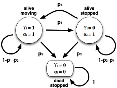
Figure 1: Schematic of transitions between stage-states for cell $i$, without interactions with other cells. Transition probabilities are denoted by $p_{1}$ through $p_{4}$

3.2 Cell movement

In the initial stages of surface colonisation, bacteria first move through a medium until they encounter and attach to a surface. This movement can be described as a series of runs and tumbles due to flagellar action [Madigan and Martinko, 2005]. A bacterium “runs” in a straight line for short distances, and then “tumbles” to change the direction of travel. If there are no external stimuli, this motion is random; directions of runs will be uncorrelated. A bacterium may move on a surface, by flagellar or twitching motility, and may exhibit a run and tumble behaviour in this case as well.

A bacterium’s direction and speed of movement through a medium or on a surface is influenced by various stimuli. The collective response to stimuli is known as taxis. For instance, chemotaxis is movement in response to chemical gradients, and phototaxis is movement in response to light gradients. Since bacteria are very small, they explore gradients with movement, keeping track of the temporal changes in signal strength instead of measuring differences in concentrations of a signal across the cell body. There is evidence that a bacterium experiencing temporal increases in an attractant decreases the frequency of tumbles, resulting in longer runs when moving up the chemical gradient. When the attractant level decreases, tumbling frequency increases, giving the bacterium more opportunities to find the desired direction.

In this model, $N$ cells, denoted by $i=1,\dots,N$, are confined to a two dimensional surface of area $A$. Each cell is modelled as a circle of radius $r$ and all cells are of equal size, i.e., $r_{i}=r_{j}=r$ $\forall$ $i,j$. As a baseline description, I assume that in the absence of any interactions between the cells, each cell’s movement can be described as an Ornstien-Uhlenbeck process:

$$d{\bf X}_{i} = {\bf V}_{i}dt$$

$$d{\bf V}_{i} = -\eta{\bf V}_{i}dt+qd{\bf W}.$$

Here $\eta$ is a drag or dissipation coefficient. However, in the rest of this paper I will assume that $\eta=0$, so that the velocities of bacteria to not dissipate. This is reasonable as bacteria can propel themselves, and overcome viscous forces. In this model, a cell moves with a random velocity at each time step, with $dW\sim N(0,1)$, and $q$ determining the change in the velocity at each time step. In this case, cells will remain randomly distributed in the space without clumping developing over time.

Next, I add simple interactions between cells and the surface. First, if two cells bump into each other (i.e. if $|{\bf X}_{i}-{\bf X}_{j}|\leq 2r$) they stick to each other and to the surface, and stop moving. This is indicated using the state variable $\phi_{i}$ which is defined as

$$\phi_{i}=\prod_{\stackrel{{\scriptstyle j=0}}{{j\neq i}}}^{N}H(|{\bf X}_{i}-{\bf X}_{j}|-2r),$$ (2)

where $H(x)$ is the Heaviside step function, so that $\phi_{i}=1$ if the $i$th cell is not overlapping any other cells, and $\phi_{i}=0$ otherwise.

I also allow individual cells to stop and stick to the surface with non-zero probability $P_{1}$, independently of interactions with other cells. The state variable $\gamma_{i,t}$ indicates if the cell is moving: $\gamma_{i,t}=1$ when the cell is moving, and $\gamma_{i,t}=0$ when the cell has stopped. Also, if $\phi_{i}=0\Rightarrow\gamma_{i,t}=0$ Then $\gamma_{i,t}=1\rightarrow\gamma_{i,t+\Delta t}=0$ with probability $P_{1}$. The transitions are then:

$$\left[\begin{array}[]{c}\gamma_{i,t+\Delta t}=1\\ \gamma_{i,t+\Delta t}=0\\ \end{array}\right]=\left[\begin{array}[]{cc}1-p_{1}&0\\ p_{1}&1\\ \end{array}\right]\left[\begin{array}[]{c}\gamma_{i,t}=1\\ \gamma_{i,t}=0\\ \end{array}\right].$$ (3)

Any cells that have stopped moving and are touching are defined to be part of a group or colony, denoted by $C_{i}$.

Next, I add an interaction between cells that are not touching. Generally, cells interact indirectly, for example by responding to chemicals released by other cells via chemotaxis. These responses can have the effect of moving the cells toward or away from each other on average, as if there were some effective force between the cells. I use a model with direct interactions in the form of forces between cells as a proxy for the behaviour we expect to see due to chemotaxis in response to chemicals released by other cells. This approach is fairly common [Lee et al., 2001, Mogilner et al., 2003]. Lee et al. (2001) examined a one dimension, continuous ODE model of chemotaxis, and showed that a non-local approximation for processes such as chemotaxis is valid if the rate of diffusion of a chemotactic signal is much faster than the rate of diffusion of the organisms. This is the case with many bacteria. Lee et al. further argue that this kind of approach facilitates learning about general properties of a system without needing to take into account the dynamics of faster scale processes. Additionally, modelling the diffusion of chemicals that are being produced and consumed by the bacteria can increase computational requirements, without providing significant gains in understanding. So instead of modelling chemotaxis explicitly, I assume that the cells in this model interact via non-local or “direct” interactions:

$$d{\bf X}_{i} = \gamma_{i,t}\phi_{i}{\bf V}_{i}dt$$

$$d{\bf V}_{i} = \frac{1}{m}F_{i}dt+qd{\bf W}.$$

Here $F_{i}$ is the force on the $i$th cell due to all other cells,

$$F_{i}=\sum_{\stackrel{{\scriptstyle i=0}}{{i\neq j}}}^{N}f_{ij}(|{\bf X}_{i}-{\bf X}_{j}|),$$ (4)

where $f_{ij}$ is the force on $i$ due to $j$, which depends only on the distance between the cells. This force can be attractive or repulsive, and differs in strength depending upon the functional form chosen for $f_{ij}$. There are various possible functional forms of non-local forces that have been used to model interactions between organisms. Many of these options are gradient type forces [Mogilner et al., 2003]. For example, Lee et al. (2001) showed that in one dimension an “effective interaction force” for chemotactic cells can take the form of a decaying exponential. Also typical are inverse power forces, with the form [Mogilner et al., 2003]:

$$F(x)=\frac{A}{x^{n}}-\frac{R}{x^{m}}.$$

I use a force of this type for the interaction between cells in this model. The value of the power law used is influenced by geometric considerations. The concentration of a chemical dispersing from a point source in three dimensions would fall off as the square of the distance to the source. I also expect that a cell will be influenced more by nearby cells than by distant cells. This is analogous to a physical force like a gravitational force. I therefore choose a functional form for the effective force between the cells that is inversely proportional to the square of the distance between cells:

$$f_{ij}=\frac{A_{i,j}}{{\bf R}_{ij}^{2}}{\bf\hat{R}}_{ij},$$ (5)

where $A_{i,j}$ is the force constant between cell $i$ and $j$ and ${\bf R}_{ij}={\bf X}_{i}-{\bf X}_{j}$ is the vector between cells $i$ and $j$. The unit vector from $i$ to $j$ is denoted by ${\bf\hat{R}}_{ij}$. If $A_{ij}>0$ the force is repulsive, and if $A_{ij}<0$ it is attractive.

This model can also be generalised to include attraction toward, or repulsion from, fixed sources of chemical signals. For instance, imagine there was an external point source of a chemical located at ${\bf X_{s}}$, and the effective force between cell $i$ and this source, which I will denote as $F_{ext}$, that has a form similar to Eqn. 5

$$F_{ext}=\frac{B}{|{\bf X}_{i}-{\bf X}_{s}|^{2}}{\bf\hat{R}}_{is}$$

where $B$ is the force constant and ${\bf\hat{R}}_{is}$ is the unit vector from cell $i$ to the chemical source. Then the total force on the $i^{th}$ cell (Eqn. 4) would become:

$$F_{i}=F_{ext}+\sum_{\stackrel{{\scriptstyle i=0}}{{i\neq j}}}^{N}f_{ij}(|{\bf X}_{i}-{\bf X}_{j}|).$$

This is similar to looking at particles undergoing Brownian motion in a field of force [Kramers, 1940]

3.3 Cell death and reproduction

The model thus far is only useful over fairly short time periods, i.e. periods much less than the average doubling time of a cell, so that the size of the population is unlikely to change. For periods longer than this, it is important to include population dynamics, in the form of births and deaths. In order to do this I use four more state variables: $\alpha_{i}$, $T_{i}$, $a_{i}$, and $\tau_{i}$ (see Table 1). The first, $\alpha_{i}$, indicates whether or not the $i^{th}$ cell is alive. Cells transition from $\alpha_{i,t}=1\rightarrow\alpha_{i,t+\Delta t}=0$ with probability $P_{2}$:

$$p(\alpha_{i,t+\Delta t}=0|\alpha_{i,t}=1)=P_{2}.$$

If $\alpha_{i}=0$, then $\gamma_{i}=0$, i.e. the cell also stops moving. Additionally, a living cell can double in a doubling period $T_{i}$. The number of times a cell has divided is the cellular age, $a_{i}$. Finally, the number of time steps since the last doubling of a cell will be denoted by $\tau_{i}$. At every time step, $\tau_{i}$ is incremented. When the time since the last doubling, $\tau_{i}$, reaches the doubling time, $T_{i}$, i.e., $\tau_{i}=T_{i}$, the cell doubles, the cellular age $a_{i}$ is incremented, and the time since the last double is reset, so $\tau_{i}=0$. With these population dynamics included, the state of the $i^{th}$ cell at time $t$ is given by:

$$\mathbf{S}_{i}(t)=\{\mathbf{X},\mathbf{V},s_{i,t},T_{i},\tau_{i},C_{i},r_{i}=r\}_{t}$$

where $s_{i,t}$ is the stage state of the cell described in Section 3.1.

The equations for the change in position and velocity over time need to be modified slightly, in order to introduce deaths into the system:

$$d{\bf X}_{i} = \alpha_{i,t}\gamma_{i,t}\phi_{i}{\bf V}_{i}dt$$ (6)

$$cd{\bf V}_{i} = \frac{1}{m}F_{i}dt+qd{\bf W}.$$ (7)

3.4 Re-spacing cells within a colony

Finally, we need to allow for interactions between individuals within a particular group or colony, $C_{i}$. Since more than one physical cell cannot occupy the same space at the same time, it is important to include at least a simple mechanism to space cells out as they reproduce within a colony.

This spacing could be approached in various ways [Picioreanu and van Loosdrecht, 2003]. Explicitly balancing forces between cells in a colony would be computationally expensive. Placing new cells at the perimeter of the colony is an alternative, but later exploration of phenotypic or genotypic variation within a colony using this framework would be impossible. Instead, I use a simple movement heuristic where overlapping cells will move away from each other, i.e., cells shove each other out of the way. This method is similar to that used in BacSim [Kreft et al., 2001]. The algorithm proceeds as follows:

1. Check if the $i$th cell overlaps with any other cells, i.e. if $\phi_{i}=0$.

2. Calculate the unit vector from the $i$th cell to each of the overlapping cells.

3. Sum these vectors, and move the $i$th cell a distance $D$ away from this new direction.

4. Repeat 1-3 over all the cells in a colony.

The distance to move the cell, $D$, will influence how quickly the colony re-adjusts itself. In general, if this distance is more than the distance required to move the $i$th cell away from its nearest neighbour, the colony will become disjoint. The choice of $D$ will therefore determine the density and compactness of the microcolonies. If reproduction stopped, the microcolonies would end up arranged such that cells would be just touching, as long as $D$ is less than or equal to the minimum overlap distance between cells. Also, if a cell from one colony overlaps with a cell from another colony at any time, these two colonies merge to form one larger colony.

4 Model Simulations

The physical space of the simulation is a two dimensional square space with reflecting boundaries. Cells are initially randomly distributed in the space, and the only sources of attraction or repulsion in the system are other cells. At each time step the simulation of the full model proceeds as follows:

1. Move all of the cells that are not already stopped.

2. Stop any of the cells that have collided with other moving cells or with stopped cells and add them to the appropriate colony.

3. If cell $i$ overlaps with cell $j$, but they are in different colonies, (i.e. $C_{i}\neq C_{j}$), then merge the colonies.

4. Consider killing any living cell w.p. $P_{2}$.

5. Consider stopping any living, moving cell w.p. $P_{1}$.

6. If any remaining living cells have $t_{i}=T_{i}$, create a new cell a distance $2r+\epsilon$ from the dividing cell, update $a_{i}$ and reset $t_{i}$. Increment $t_{i}$ for any cells that do not divide.

7. Within each colony, re-space cells using the shoving algorithm.

Sub-models can be formulated by excluding portions of the above algorithm or varying parameters in order to see what the effects of various processes have upon the distributions of cells in space.

4.1 Model with clumping and direct interactions between cells.

First I explore a sub-model where cells can clump and sense each other, but cannot reproduce or die, and do not re-space themselves within a colony. All simulations presented in this section consist of 5000 cells initially distributed randomly in a 500 x 500 square space (in units of the cell radius). All simulations began with the same initial distribution. I also set $q=1$, and assume reflecting boundaries.

Under this model, the distribution of colony sizes after all cells have stopped moving for three values of the stopping probability, $P_{1}$ with no forces between cells ($A_{i,j}=0$) are shown in Figure 2. Increasing the stopping probability mainly acts to shift more cells from colonies of size 2 into colonies of size 1 (as can be seen when comparing Figure 2a and b). However, as $P_{1}$ gets much larger, the proportion of individual cells stopping without running into other cells increases. This results in the formation of more colonies of size 1, and a decrease in the number of colonies of size $>2$. (Figure 2c).

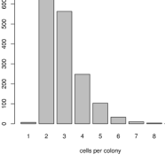
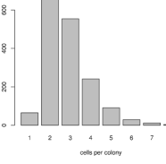
(a)	(b)

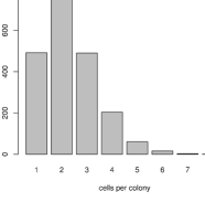
(c)

Figure 2: Distribution of colony sizes for model with stopping and clumping, but no interactions between cells for three values of the stopping probability, $P_{1}$ (a) $P_{1}=0.0001$ (b) $P_{1}=0.001$ (c) $P_{1}=0.01$, after all cells have stopped moving.

In Figure 3 I show the final distributions colonies and colony sizes for attractive forces, (Figure 3 a), no forces (Figure 3 b), and repulsive forces (Figure 3 c). For the attractive case the force constant $A=-10$, and for the repulsive case $A=10$. Notice that each of these models exhibits distinctive distributions of colony size (numbers of cells in a colony). In particular, when there are attractive forces between cells, the colonies are much more likely to be large, and the distribution exhibits a longer and heavier right hand tail. When the cells repulse the colonies are smaller than when they only interact randomly.

A simple $\chi^{2}$ test can be used to confirm that the three cases explored here (i.e. attractive, no force, and repulsive) do in fact result in distinct distributions. I define the case of motion without forces to be the “expected” distribution. The first null hypothesis, $H_{0}$, is that the distribution from the attractive case is the same as that of the the distribution found when there were no forces present. The alternative hypothesis, $H_{1}$, is that they are not equal. Since the $\chi^{2}$ test requires at least five counts in any bin to give a good result, it is necessary to re-bin each distribution into 7 bins: $\{1,2,3,4,5,6,7+\}$. This corresponds to 6 degrees of freedom in the test. A significance level of 0.001 corresponds to a $\chi^{2}$ value of 22.547. For this first test, the $chi^{2}$ value is $\chi^{2}=2448.036$ leading to a rejection. For the second test, testing the hypothesis that the repulsive distribution is the same as the no force (expected) distribution, I find $\chi^{2}=1029.437$, leading to another rejection. Thus as the 0.001 level, I reject the hypotheses that the attractive and repulsive distributions are the same as the random case.

These three cases can be viewed as representative of the types of clumping that might be observed in a bacterial system. For instance, in a system where bacteria attract via chemotaxis, we might see distributions of microcolonies similar to those shown in Figure 3a. However, if the chemotaxis system is disrupted, for instance by some chemical additive or by genetic manipulation, then the new system might look more like what is shown in Figure 3b. If on the other hand, the system is manipulated so that the chemotaxis system is reversed, so cells move away from each other, the system would appear more like what we see in Figure 3c.

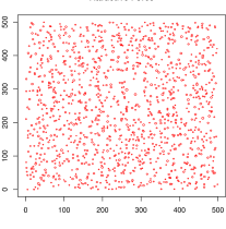
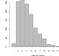
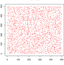
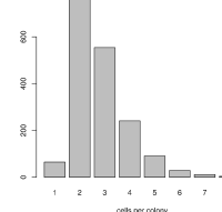
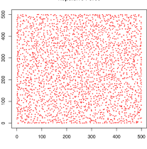
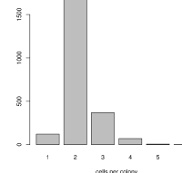
Figure 3: Distribution of colony locations and sizes with and without interactions between cells with $P_{1}=0.001$. (TOP) Attractive forces between cells; (MIDDLE) no forces between cells; (BOTTOM) repulsive forces between cells.

4.2 Model with clumping, direct interactions, and births and deaths

Next I explore a sub-model that includes all portions of the full model except shoving within a colony. All simulations presented in this section consisted of cells initially distributed randomly in a 500 x 500 square space (in units of the cell radius). Parameter settings for the simulations are shown in Table 2.

Parameter	Value
$N_{initial}$	250
$t_{final}$	1000
$P_{1}$	0.001
$P_{2}$	0.00005
# replicates	50

Table 2: Parameter settings for simulations of model with clumping, direct interactions, and births and deaths

In Figure 4 I show visualisations of the frequencies of colony sizes cells aggregated over 50 replicates for 3 different doubling times (200 steps, 300 steps or 400 steps), three force constants ($A=-10$, $A=0$, and $A=10$ for the attractive, no force, and repulsive cases, respectively), and a no movement case.

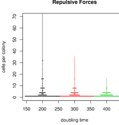
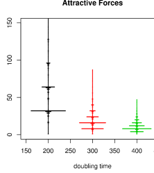
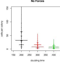
Figure 4: Alternative histograms of final colony size. The width of the horizontal bars correspond to the counts in the histogram.

Except for the case of repulsive forces, where cells continue moving for longer and form smaller colonies, the spacing between the major peaks of the distribution corresponds to $2^{d}$ where $d=\left\lfloor\frac{T_{i}}{t_{tot}}\right\rfloor$, where $t_{tot}$ is the total run time, $T_{i}$ is the doubling time, and $\lfloor\cdot\rfloor$ denotes the floor function, which returns the largest integer smaller than or equal to the argument. This value of $2^{d}$ also usually corresponds to the mode or to the second largest peak of the distribution. For example, for $T_{i}=200$, $d=5$ so the largest peak is at $2^{5}=32$ and other major peaks are spaced at $\sim 32$ individuals apart (e.g. in Figure 4 top left panel). The other simulations show similar patterns, with variability being caused by the interactions between individual cells, and stochastic deaths. There is additional variability in the simulation with $T_{i}=300$ and $T_{i}=400$ since these correspond to non-integer values of $\left(\frac{T_{i}}{t_{tot}}\right)$. In these cases, all cells reproduce at least $d$ times, but a proportion will reproduce $d+1$ times . However, the pattern of major peaks is approximately $2^{d}$ times the distribution of colony sizes for model $M_{2}$ (interactions without births and deaths) as shown in Figure 3.

4.3 Full model

Finally, I examine the behaviour of the full model. Examples of cell distributions on the surface before and after implementing the shoving heuristic appear in Figures 5 and 6. For the four simulations generating these distributions, the value of the shoving distance $D$ was set to $\frac{1}{4}$ of the distance between the $i$th cell and its nearest neighbour. We can see that colonies are more likely to merge when their members spread themselves out. This should increase the proportion of large colonies that are observed. For cases where the cell density is low, we can expect this effect to be small. However for larger populations, this effect could be significant. For the repulsive case, the spreading also increases the magnitude of the edge effects when the area of interest is small or cell density is high (Figure 6).

In order to explore the effect of the spreading on the observed distributions of colony sizes, I ran simulations using the same parameter values as in the previous section (shown in Table 2). In Figure 7, I show plots of the distribution of final colony sizes aggregated over 50 runs. Notice that these distributions are very similar to those without shoving (Figure 4) except that the tails are slightly longer and heavier. For long doubling time (i.e. $T=400$) the effect is minimal, since the final population size is smaller.

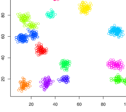
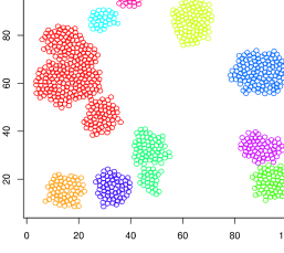
(a)	(b)

Figure 5: Example of cell distribution and colony membership (cells in a colony are the same color) before and after implementation of the spreading heuristic. Both simulations were run starting from the same initial cell distribution of 30 cells. Simulation parameters: $T_{i}=200$, force=-10, $prob_{death}=0.00001$, $prob_{stop}=0.0005$, $T_{final}=1000$.

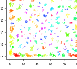
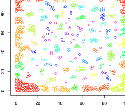
(a)	(b)

Figure 6: Example of cell distribution and colony membership (cells in a colony are the same color) before and after implementation of the spreading heuristic, but with repulsive forces between the cells. Both simulations were run starting from the same initial cell distribution of 30 cells. Simulation parameters: $T_{i}=200$, force=10, $prob_{death}=0.00001$, $prob_{stop}=0.0005$, $T_{final}=1000$.

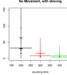
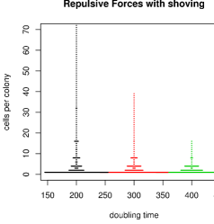
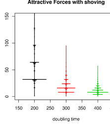
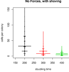
Figure 7: Histogram of final colony sizes for full model. Parameter settings are the same as for the simulations for model without shoving.

5 Discriminating between models

In order for this model formulation to be useful in approaching data, it must be possible to discriminate between distributions of colony sizes with different parameter settings. In Section 4.1 I approached this issue by using a $\chi^{2}$ hypothesis test to check if two distributions are the same. This method cannot be used for discriminating between the distributions obtained for models that include reproduction because the number of counts of colony sizes is too low (and often zero) in many bins, rendering the $\chi^{2}$ test is invalid. The data also cannot be re-binned without loss of information about the structure of the distribution. Instead, a different measure of the distance between the histograms is necessary.

5.1 Jackknife hypothesis test

Let $H_{i}$ for $i=1,\dots,n$ be histograms summarising $n$ simulations from the model with a fixed set of parameters. Aggregating these $n$ histograms into a single histogram, denoted by $H_{a}$, gives an approximation of the target distribution of groups sizes. Imagine that some new “data” histogram, $H_{data}$, is observed. We would like to perform an hypothesis test to see if $H_{data}$ is from the same model that generated the $H_{i}$’s. To do this we need a test statistic and a way to calculate the sampling distribution of this statistic. A simple choice for a test statistic is to calculate the Minknowski Distance between the data and the aggregate histograms. The $L_{p}$ Minknowski distance between $H_{1}(m;T)$ and $H_{2}(m;T)$, where $m$ is the number of bins in the histogram and $T$ is the total number of counts, is given by

$$D(H_{1},H_{2})=\left(\sum_{x=1}^{n}\left|H_{1}(x;T)-H_{2}(x;T)\right|^{p}\right)^{(1/p)}.$$ (9)

When $p=2$, this distance gives the Euclidian distance.

Once a test statistic has been chosen, its sampling distribution needs to be derived. When the sampling distribution is not known in closed form (either exactly or approximately) it can be calculated empirically using, for example, a delete-1 jackknife [Shao and Tu, 1995]. Let $d_{i}=D(H_{i},H_{a,-i})$ be the distance from the $i$th histogram to the aggregated histogram of the $n-1$ remaining realisations, denoted by $H_{a,-i}$. Then, the empirical CDF of the test statistic is

$$F(d)=p(D\leq d)\approx\frac{1}{n}\sum_{i=1}^{n}1_{[[d_{i}<d]]},$$

where $1_{[[\cdot]]}=1$ if $[[\cdot]]$ is true and zero otherwise. Let $d_{1-\alpha}$ be the rejection threshold corresponding to the $(1-\alpha)$ quantile of the CDF. When $H_{data}$ is observed I can calculate the distance from the data to the full aggregate histogram $H_{a}$:

$$d_{data}=D(H_{data},H_{a})$$

and then compare $d_{data}$ with $d_{1-\alpha}$. If $d_{data}>d_{1-\alpha}$ I reject the hypothesis that the models generating $H_{1},\dots,H_{n}$ and $H_{data}$ are the same. It can be shown that this test has a Type I error of approximately $1-\alpha$ when $n$ is large. A similar hypothesis test could also be constructed using either a delete-$d$ jackknife or a bootstrap method [Shao and Tu, 1995].

5.2 Hypothesis test on simulated data

Suppose I have $n=50$ realisations of final colony size from the full model for the following parameter sets: attractive ($A=-10$), repulsive ($A=10$), no force ($A=0$), and no movement ($A=0$ and $P_{1}=1$), all with doubling time $T=300$. The aggregate distributions are shown in Figure 7. I will refer to these as the reference models or distributions. In Table 3 I show the maximum, 95% quantile, 75% quantile, and mean of the distributions of Euclidian distances ($\{d_{i}\}_{i=1}^{n}$) for these cases. The value of the 95% quantile (or similarly the $(0.95)n^{th}$ order statistic) serves as a rejection threshold for hypothesis tests comparing new data with the reference models.

Model	Max	95% Quantile	75% Quantile	Mean
Attractive ($A=-10$)	16.59	12.94	11.10	9.67
Repulsive ($A=10$)	74.49	48.03	33.92	27.15
Random ($A=0$)	35.63	20.75	15.11	12.95
No Movement	17.65	17.23	13.02	10.52

Table 3: Maximum, 95% Quantile, 75% Quantile, and Mean of the distributions of distances $d_{i}$ for 4 parameter settings of the full model (reference models). Parameters are as in 2, with doubling time $T=300$, except for the no movement case which has stopping probability $P_{1}=1$.

I conducted four additional simulation runs, one for each of the attractive, repulsive, random, and no movement cases. I then calculated the Euclidian distance from each of these individual runs to the reference histograms ($d_{data}$). These appear in Table 4. The rows correspond to reference histograms, and columns to individual runs. The distance from the individual run to the reference distribution generated from the same set of parameters is indicated in bold face. Notice that the bold value is the lowest distance in each column. These bold distances are all lower than the corresponding 95% quantile noted in Table 3, so I cannot reject the hypothesis that the individual run is from the corresponding reference model. Distances to all other reference distributions are higher than the respective 95% quantile. In these cases, the hypothesis that the individual run is from the same distribution as the reference model is rejected.

Model	Attractive	Repulsive	Random	No Movement
Attractive ($A=-10$)	6.81	894.0	49.16	63.61
Repulsive ($A=10$)	102.5	23.35	166.3	189.5
Random ($A=0$)	27.74	877.8	16.76	40.76
No Movement	43.52	1020	58.20	16.80

Table 4: Distances from new individual simulations to the aggregate distributions ($d_{data}$). The new data sets are simulated using the same parameter settings as the four reference models.

The first set of comparisons presented above indicates that the method is well-calibrated because we accept and reject where we expect to. However, there is still the possibility that we would not be able to distinguish between models that have similar (but not exactly the same) parameters. To explore this, I ran ten additional simulations, this time with at least one of either the force constant ($A$) or the the doubling time ($T$) different from any of the reference models. First, I looked at variation in the force constant only. In Table 5 I show distances between the reference models and individual runs with five different values of $A$, ranging from $A=5$ (mild repulsion) through $A=-8$ (moderate attraction). Notice that all of these distances are in the rejection region. Moreover, most of them are also significantly larger than maximum of the within model distances, $d_{i}$.

Model	$A=5$	$A=0.5$	$A=-2$	$A=-5$	$A=-8$
Attractive ($A=-10$)	582.5	40.17	65.57	22.47	58.80
Repulsive ($A=10$)	131.0	183.4	156.9	135.1	129.3
Random ($A=0$)	559.6	68.00	92.15	25.34	81.63
No Movement	682.4	97.07	110.1	35.83	99.00

Table 5: Distances from new individual simulations to the aggregate distributions ($d_{data}$). The new data sets are simulated using the same parameter settings as the four reference models, except for the force constant $A$.

Next, I changed the doubling time, so that $T=250$ and calculated the distances from these new runs to the reference distributions (Table 6). Here again, all of the distances fall outside of the non-rejection region, except for the individual repulsive ($A=10$) run (Table 6 in bold face). This is likely because the individual cells move for much longer and form smaller groups regardless of the doubling time, so distinguishing between two repulsive cases with similar doubling times is likely to be difficult.

Model	$A=-10$,	$A=10$,
	$T=250$	$T=250$
Attractive ($A=-10$)	42.65	1169
Repulsive ($A=10$)	102.0	38.76
Random ($A=0$)	61.39	1152
No Movement	78.20	1344

Table 6: Distances from new individual simulations to the aggregate distributions ($d_{data}$). The new data sets are simulated using the same parameter settings as the attractive and repulsive reference models, except with $T=250$.

Finally, I calculated distances between individual runs and the reference distributions (with both $A$ and $T$ different from those used to generate the aggregate distributions – Table 7). Again, all of these distances are large enough to reject the hypothesis that the individual runs were generated from the model corresponding to the aggregate distributions.

Model	$A=-5$,	$A=5$,	$A=60$,
	$T=250$	$T=250$	$T=450$
Attractive ($A=-10$)	64.21	649.3	578.4
Repulsive ($A=10$)	139.1	200.3	51.02
Random ($A=0$)	88.89	622.7	574.6
No Movement	107.33	775.6	663.8

Table 7: Distances from new individual simulations to the aggregate distributions ($d_{data}$). The new data sets are simulated using the same parameter settings as the four reference models, except for $A$ and $T$ (as indicated in the table).

6 Fitness of bacteria in microcolonies

This analysis of models of microcolony formation presented thus far neglects the question: why do bacteria employ a strategy that results in a particular microcolony size? We would expect that the strategies must be related to the fitness of the bacteria. For instance, if bacteria repel each other, there must be an advantage to small group size, at least initially, perhaps because of better access to nutrients and increased reproductive rates. On the other hand, aggregation would provide some advantage that favours large groups, such as protection from predation [Matz et al., 2005].

Mortality rates are often size dependent [Lorenzen, 1996, McGurk, 1986]. For instance, a traditional model for a size dependent mortality rate, $m(L)$, is

$$m(L)=m_{1}+\frac{m_{2}}{L}$$ (10)

where the length of the organism is $L$, $m_{1}$ is some constant mortality, and $m_{1}+m_{2}$ gives the mortality rate of the organism at length $L=1$. For a bacterial microcolony, I use this form for the average mortality of a single bacterium in a group, where $L$ is the diameter of the group (assuming the group is approximately circular). Measuring the group size as a multiple of the diameter of a cell, $m_{1}+m_{2}$ is the mortality rate of a single bacterium and $m_{1}$ is the mortality rate of bacteria in a large group.

Living in a microcolony or biofilm may improve survival, but since resources are limited, living in a group is likely to decrease the rate of reproduction, or increase the doubling time. For instance I assume a simple relationship between group size and doubling time, $T$, such that

$$T(L)=T_{1}+T_{2}L^{\gamma}.$$ (11)

I examine the case of $\gamma=1$. In this case, $T_{1}+T_{2}$ is the doubling time of a single bacterium.

Johnson and Mangel (2006) propose a simple model of bacterial fitness when bacteria age, i.e. experience limited reproduction. In this model the fitness of a bacterium, $\tilde{r}$ is

$$\tilde{r} \approx\frac{\ln{2}}{T}-m-\frac{\epsilon}{T}$$ (12)

where $m$ is the mortality rate, $T$ is the doubling time, and $\epsilon=\frac{2^{-a_{max}}}{\ln{2}+a_{max}2^{-a_{max}}}$, where $a_{max}$ is the maximum number of times a bacterium can double. Using Eqns. (10) and (11) for $m$ and $T$ in Equation (12) gives the fitness of the bacterium as a function of the group size $L$

$$\tilde{r}(L)\approx\frac{b}{T_{1}+T_{2}L}-m_{1}-\frac{m_{2}}{L}$$ (13)

where $b=\ln{2}-\epsilon$. The optimal group length $L^{*}$ will maximise the fitness, so that $\frac{d\tilde{r}(L^{*})}{dL}=0$. Solving for $L^{*}$ gives

$$L^{*}_{\pm}=\frac{-T_{1}\pm T_{1}\left(\frac{b}{m_{2}T_{2}}\right)^{\frac{1}{2}}}{T_{2}-\frac{b}{m_{2}}}.$$

For this to make sense as a length, $L^{*}$ must be positive. The first of these solutions

$$L^{*}_{+}=\frac{-T_{1}+T_{1}\left(\frac{b}{m_{2}T_{2}}\right)^{\frac{1}{2}}}{T_{2}-\frac{b}{m_{2}}}$$

cannot yield positive group lengths. The second solution

$$L^{*}_{-} =\frac{-T_{1}-T_{1}\left(\frac{b}{m_{2}T_{2}}\right)^{\frac{1}{2}}}{T_{2}-\frac{b}{m_{2}}}$$

$$=\frac{T_{1}+T_{1}\left(\frac{b}{m_{2}T_{2}}\right)^{\frac{1}{2}}}{\frac{b}{m_{2}}-T_{2}}$$ (14)

corresponds to a positive solution if $T_{2}<\frac{b}{m_{2}}$. If I define $\omega=\frac{b}{m_{2}T_{2}}$, Equation (14) becomes

$$L^{*}=\frac{T_{1}}{T_{2}}\left(\frac{\omega^{\frac{1}{2}}+1}{\omega-1}\right)$$ (15)

where $\omega>1$. Notice that the optimal group size does not depend upon the size independent mortality rate $m_{1}$, since this only shifts the fitness by a constant.

If the group of bacteria is approximately circular, and the area covered by the groups is approximately the number of cells in the group, $N$, multiplied by the area covered by a single cell, then the diameter of the group scales as $N^{\frac{1}{2}}$. The optimal number of individuals in a group is then approximately

$$N^{*}\approx(L^{*})^{2}=\left(\frac{T_{1}}{T_{2}}\left(\frac{\omega^{\frac{1}{2}}+1}{\omega-1}\right)\right)^{2}.$$ (16)

Very large values of $N^{*}$ will be optimal if at least one of two conditions holds. The first is that $T_{2}<<T_{1}$, i.e., larger group sizes only have a small effect on the doubling rate, so that the ratio of $T_{1}$ to $T_{2}$ will be large. The optimal group size will also be large when $\omega\approx 1$ which corresponds to $m_{2}\approx\frac{b}{T_{2}}$. This means that if the doubling time increases quickly with group size, i.e. $T_{2}$ is large, the group must provide significant protection for large group sizes to be optimal. If $m_{2}$ is due to predation, for instance, then the threat would not be constant in time, and the optimal group size would depend on predators being present in the environment. This requires that bacteria be able to sense that there is danger and modify their behaviour accordingly. V. cholerae appear to exhibit this behaviour. Matz et al. [Matz et al., 2005] studied biofilm formation in V. cholerae in the presence of predatory protozoa. They found that bacteria living in biofilms are protected from protozoa compared to those living in planktonic state, and that bacteria in the biofilm produce compounds which inhibit the growth of the protozoa. They also found that if there is predation of the planktonic state, biofilm formation is significantly enhanced compared to growth without predation. The bacteria appear to regulate these various responses to the protozoa via quorum sensing.

The calculation of optimal group size here gives a way to estimate how strong predation must be in order for the biofilm state to be preferred, and estimate what levels of predation and what group sizes are necessary to initiate quorum sensing. On the other hand, if the mortality rates of individual bacteria and large groups can be measured and the doubling time for planktonic bacteria is known (as in the experiments by Matz et al.), the values of $T_{2}$ required to select for large group sizes could be calculated. These calculations also indicate what types of environments (presence/absence of predators, nutrient limitation, etc.) are likely to be correlated with the different types of surface movements explored in the IBM introduced in this paper. For instance, if $T_{2}$ is large, and the risk of predation is low ($m_{2}$ is small), then repulsive forces, which results in smaller group sizes, would be predicted to be prevalent. However, attraction between individuals, which would allow larger groups to be formed faster, would be optimal if the risk of predation is high.

To make this more concrete, I calculate approximate values of the parameters using the experimental data from [Matz et al., 2005]. In experiments lasting for 72 hours, Matz et al. found that with a planktonic predator, the population of planktonic bacteria was reduced by $>94\%$. On the other hand, the biofilm population was unaffected by a surface predator. I assume a doubling time for planktonic bacteria ($T_{1}+T_{2}$) of $0.34$ hours (about 20 minutes). Since $T_{2}$ is unlikely to be very small (as biofilms tend to decrease the diffusion of nutrients to many of the members) and the system favours very large groups when predators are present (as was indicated by increased biofilm formation in the presence of the planktonic predator), I also assume that $T_{2}\approx\frac{\ln{2}}{m_{2}}-small$, so that $L^{*}$ is very large. The estimated values of the parameters are then: $m_{1}\approx 0.0001$, $m_{2}\approx 2.079$, $T_{1}\approx 0.0068$, and $T_{2}\approx 0.3332$, corresponding to an optimal group size of $L^{*}=3200$ or $N^{*}\approx 10^{7}$. In Figure 8 a & b I show $\tilde{r}$ as a function of $L$ for these parameters, with the optimal group size indicated on the curve. Notice that for this case, the fitness is always less than one, and the population will decline, whereas if $m_{2}$ is reduced a small amount (Figure 8 c) the fitness would be positive. This is because of the value of the constant mortality $m_{1}$. If this mortality were zero, then the population in a large group would be stationary ($\tilde{r}=0$).

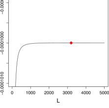
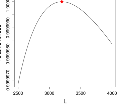
(a)	(b)

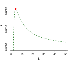
(c)

Figure 8: (a) Fitness of bacteria. $\tilde{r}$ as a function of groups size, $L$ for parameters estimated from data in Matz, et al. $m_{2}=2.079$ with $T_{2}=0.3334$, $m_{1}=0.0001$, $T_{1}=0.0068$, $b=\log 2$. $L^{*}$ is indicated with a red point. (b) Close-up of (a) near the optimal group size, $L^{*}$. The y-axis here indicates relative fitness Relative fitness ($\tilde{r}/\tilde{r}_{max}$) (c) $r$ vs. $L$ for parameters estimated from data in Matz, et al., except with $m_{2}=2.06$.

In Figure 9 I show plots of $\tilde{r}$ as a function of $L$ varying $m_{2}$ (Figure 9 a) and varying $T_{2}$ (Figure 9 b) with the other parameter values set to those estimated here. For the optimal group size to be reduced to $N^{*}\approx 1$, the predation mortality must be decreased to about $m_{2}=2.02$, a reduction of only $\approx$ 3%. In otherwords, this model predicts that a small reduction in mortality of planktonic bacteria would result in individual bacteria being more prevalent (top three lines in Figure 9 a). If the mortality, $m_{2}$, remains constant, a decrease in the size dependent mortality rate to $T_{2}\approx 0.25$ gives a smaller optimal groups size (in this case $N^{*}\approx 4$), so small groups should be more prevalent. Notice that when the optimal group size is small the fitness surface is sharply peaked around the optimal value, so there would be little variability in clump sizes. On the other hand, as the optimal group size increases, the fitness surface flattens out. This is especially obvious in Figure 8 b, where the difference in fitness between the maximum fitness at $L^{*}=3200$ and the fitness of a groups of size $L=2500$ is on the order of $10^{-9}$. This indicates that there would be more variability in clump sizes under these conditions, since even groups with sizes that are far from the optimal will have similar fitness.

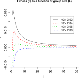
(a)

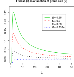
(b)

Figure 9: Fitness of bacteria as a function of groups size for (a) 4 values of $m_{2}$ with $T_{2}=0.3334$ and (b) 4 values of $T_{2}$ with $m_{2}=2.08$. Values of other parameters are: $m_{1}=0.0001$, $T_{1}=0.0068$, $b=\log 2$.

7 Discussion

Individual Based Models have traditionally been used to explore how the behaviour of individuals combine to create large scale or group patterns. Instead of encoding a particular large scale pattern explicitly into the dynamics of the system, IBMs seek to identify individual behaviours that can generate emergent properties or patterns.

The formation of bacterial communities, such as biofilms, has major implications for survival and fitness of bacteria. To understand patterns of group formation in these organisms we must gather information about how behaviour of individual bacteria influences these patterns. The IBM presented here is one way to approach this problem.

This model provides useful qualitative and quantitative predictions of how the size of microcolonies depends on the behaviour of the cells. Qualitative results include insight into how inter-cellular interactions tend to influence the mean colony size, maximum colony size, and heaviness of distribution tails. For example, repulsive forces result in smaller mean colony sizes, with short tails, whereas attractive forces increase the likelihood of larger colonies, as well the maximum observed colony size. We also expect that if predators are present, individuals should aggregate more quickly.

Quantitatively, the model predicts that the spacing between peaks is proportional to the expected number of doublings in the observation period. The results of this model also indicate that although the patterns of colony size are complicated, different behaviours result in patterns that are statistically different. This enables us to conclude that groups of individuals are exhibiting different behaviour simply by comparing the patterns of group sizes. The distinctness of the patterns means that this model would be useful for making quantitative predictions, and for inferring from empirical data the strategies employed by bacteria in the initial stages of biofilm formation.

When studying bacterial biofilm formation, we are often interested in genes that are important for the development of the biofilms. In laboratory experiments, genes that are thought to be involved in attachment or biofilm formation are deleted or mutated. Bacteria with these modifications are then grown in vitro to see if they can still form biofilms or produce certain substances. However, often the particular functions of the genes involved are unknown. Even if the function is known, why that gene is important or how it influences community structure may be unknown. For instance, genes that are believed to influence chemotaxis and motility in V. cholerae are also important to biofilm formation. However, how these genes mediate inter-cellular interactions and biofilm formation is well not understood. As a first step, we are interested in learning if these genes may be playing a part in the initial stages of biofilm formation. The model presented here provides a framework for exploring these kinds of questions.

For instance, imagine a flow cell experiment. The flow cell is first inoculated with bacteria, which are allowed a short amount of time to form initial attachments to the surface. After a short time has elapsed, the flow cell is flushed so that any bacteria not already attached to the surface are removed. Initial images could be taken to determine the approximate initial cell density, although this is likely not necessary, unless the initial densities are either very high or very low. Then fresh medium is allowed to flow through the flow cell. The remaining bacteria reproduce and/or move around on the surface. Images can be taken at later times, and the approximate number of cells per colony can be recorded. These data can then be compared with model predictions. This would provide information about which of the models presented best matches the results of the experiment as well as what type of behaviour the bacteria are exhibiting, i.e. if they are attracting via chemotaxis, or moving along the surface at all. Experiments involving bacteria with certain mutations, such as one that completely removes the ability of a bacteria to produce a flagellum or a mutation that alters a chemotaxis system, could be used to pin down estimates of parameters such as the doubling time or effective force of attraction/repulsion, and indicate which genes are correlated with specific behaviours.

Before comparing the simulated distributions with empirical data, it could be useful to estimate empirically the probability of making a type II error (i.e. accepting the hypothesis that the data is generated by a particular model, when the data was actually generated by another model). This would require simulating large sets of data from each model, and then comparing the “data” with the various reference distributions using the jackknife type hypothesis test described earlier.

Fairly simple extensions and modifications of the models explored here could be used to explore other kinds of bacterial communities. For instance, by adjusting the shoving parameters, the clumpiness and density of the communities can be manipulated, which may give insight into what behaviours are involved in determining colony morphology. Allowing shoving to shape the surface attached groups in three dimensions could also be useful in this regard. One way to do this would be to combine the IBM explored here with BacSim (or some other biofilm modelling tool) to explore how colony and biofilm structures are influenced by the behaviours of individuals during initial surface colonisation.

Another important extension would be to explore how different functional forms for the interaction forces between individuals influences the distributions of colony sizes. In particular, modelling chemotaxis explicitly together with an analysis of what functional form of direct forces is the best approximation for chemotaxis would be useful.

The model could also be easily expanded to include multiple types of bacteria, or genotypic and phenotypic variation between individuals. For instance, one study on Pseudomonas aeruginosa, conducted by Klausen, et al. (2003) looked at aggregation and biofilm formation when individuals were marked with one of two florescent markers (either blue or green). They concluded that because bacterial colonies were not 50-50 blue-green, the bacteria were not aggregating on the surface. The IBM presented here could be used to explore how the size and composition of groups varies depending on how individuals interact with other individuals (of the same and different colors) more explicitly, in order to draw more concrete conclusions about the behaviour of these bacteria.

8 Acknowledgements

This work was supported by a UC Presidents Dissertation Year Fellowship. Thanks to Marc Mangel for comments on earlier drafts and to Robert Gramacy for advice on statistical methods.

References

- Branda et al., 2005 Branda, S. S., Vika, Å., Friedmanb, L., and Kolter, R. (2005). Biofilms: the matrix revisited. TRENDS in Microbiology, 13(1):20–26.
- Davey and O’Toole, 2000 Davey, M. E. and O’Toole, G. A. (2000). Microbial Biofilms: from Ecology to Molecular Genetics. Microbiol. Mol. Biol. Rev., 64(4):847–867.
- Davies et al., 1998 Davies, D. G., Parsek, M. R., Pearson, J. P., Iglewski, B. H., Costerton, J. W., and Greenberg, E. P. (1998). The Involvement of Cell-to-Cell Signals in the Development of a Bacterial Biofilm. Science, 280(5361):295–298.
- Grimm and Railsback, 2005 Grimm, V. and Railsback, S. F. (2005). Individual-based Modeling and Ecology. Princeton University Press, Princeton, NJ.
- Gueron and Levin, 1995 Gueron, S. and Levin, S. A. (1995). The Dynamics of Group Formation. Mathematical Biosciences, 128:243–264.
- Gueron et al., 1996 Gueron, S., Levin, S. A., and Rubenstein, D. I. (1996). The Dynamics of Herds: From Individuals to Aggregations. Journal of Theoretical Biology, 182:85–98.
- Hahn and Höfle, 2001 Hahn, M. W. and Höfle, M. G. (2001). Grazing of protozoa and its effect on populations of aquatic bacteria. FEMS Microbiology Ecology, 35:113–121.
- Heydorn et al., 2002 Heydorn, A., Ersboll, B., Kato, J., Hentzer, M., Parsek, M. R., Tolker-Nielsen, T., Givskov, M., and Molin, S. (2002). Statistical Analysis of Pseudomonas aeruginosa Biofilm Development: Impact of Mutations in Genes Involved in Twitching Motility, Cell-to-Cell Signaling, and Stationary-Phase Sigma Factor Expression. Appl. Environ. Microbiol., 68(4):2008–2017.
- Jefferson, 2004 Jefferson, K. K. (2004). What drives bacteria to produce a biofilm? FEMS Microbiology Letters, 236:163–173.