Frequency and phase synchronization of two coupled neurons with channel noise

Abstract

We study the frequency and phase synchronization in two coupled identical and nonidentical neurons with channel noise. The occupation number method is used to model the neurons in the context of stochastic Hodgkin-Huxley model in which the strength of channel noise is represented by ion channel cluster size of neurons. It is shown that channel noise allows the two neurons to achieve both frequency and phase synchronization in the regime where the deterministic Hodgkin-Huxley neuron is unable to be excited. In particular, the identical channel noises lead to frequency synchronization in weak-coupling regime. However, if the coupling is strong, the two neurons could be frequency locked even though the channel noises are not identical. We also show that the relative phase of neurons displays profuse dynamical regimes under the combined action of coupling and channel noise. Those regimes are characterized by the distribution of the cyclic relative phase corresponding to antiphase locking, random switching between two or more states. Both qualitative and quantitative descriptions are applied to describe the transitions to perfect phase locking from no synchronization states.

I INTRODUCTION

The synchronization phenomena have been widely studied in neural systems in past decades kurth ; Gray2 ; Robert ; Pinto ; li02 . Experiments show that the synchronization of coupled neurons could play a key role in the biological information communication of neural systems Gray2 . Recent research also suggests that synchronization behavior is of great importance for signal encoding of ensembles of neurons. Especially the phase synchronization may be important in revealing communication pathways in brain Fitzgerald . Studying the synchronization of a pair of coupled neurons has attracted large amounts of research attention. In order to understand the dynamical properties of a neural network, it is important to characterize the relation between spike trains of two neurons in the network Uchida . What’s more, studies show that noise enhances synchronization of neural oscillators. For example, the identical neurons which are not coupled or weakly coupled but subjected to a common noise may achieve complete synchronization. Actually, this is a general results for all the dynamical system pikovsky1 ; Maritan ; pikovsky2 ; zhou ; Herzel . Both independent and correlated noises are found to enhance phase synchronization of two coupled chaotic oscillators below the synchronization threshold Yuqing Wang ; Istvan .

Among large population of neurons, different neurons are commonly connected to other group of neurons and receive signals from them. As a result of integration of many independent synaptic currents, those neurons receive a common input signal which often approaches a Gaussian distribution Changsong Zhou . Therefore, noise was usually considered as external and introduced by adding to the input variables. However, recent work found that the random ionic-current changes produced by probabilistic gating of ion channels, called channel noise or internal noise, also play an amazing role in single neuron’s firing behavior and information processing progress Hille ; White1 ; Freedman . Besides, Casado has showed that channel noise can allow the neurons to achieve both frequency and phase synchronization Casado1 ; Casado2 . This finding suggests that channel noise could play a role as promoter of synchronous neural activity in population of weakly coupled neurons. However, Casado didn’t give a quantitative description of the results.

The magnitude of the ion channel noise is changed via the variation of the channel cluster size of neurons. It implies that synchronization in neural system is also restricted by the channel cluster size of neurons. Actually, the cluster size of ion channels embedded in the biomembrane between the hillock and the first segment of neurons determines whether the neuron fires an action potential. The channel cluster size of this region is different for different neurons or for different developing stages of a neuron. With the decreasing of ion channel cluster size, ion channel noise would be induced thus the firing behavior of neurons would be greatly changed (for review see RefWhite1 ). It is natural to ask to what extent the change of the channel cluster size affect the collective activities of neuron ensembles. For this purpose, we investigated the effect of ion channel cluster sizes (i.e, channel noise ) of neurons on synchronization of two coupled stochastic Hodgkin-Huxley (HH) neurons in this paper.

Here we adopted a so called occupation number method rather than the Langevin method Casado had used to describe the single neuron for two reasons. First, the Langevin approach has been proved could not reproduce accurate results for small and large cluster sizes. Second, occupation number method gives a direct relation between channel cluster size of neuron and its firing behavior, and it’s the fastest method for a given accuracy Shangyou Zeng . The main goal of our work is to explore what role the channel noise might play in the synchronization of two coupled neurons. We try to give qualitative as well as quantitative descriptions of the result. The practical meaning of our study is obvious, since the channel cluster size of neurons can be regulated by channel blocking experimentally Schmid , our study may provide a possible way to control neural synchronization.

This paper is organized as follows. In section II, the occupation number method of stochastic Hodgkin-Huxley neuron is introduced and the firing behaviors of neurons with different channel cluster sizes are demonstrated. In the following sections, we explored the combined effect of coupling strength and cluster size on the synchronization behaviors of two neurons with an electrical synaptic connection. Section III is devoted to frequency synchronization. The phase synchronization of identical and nonidentical neurons are discussed in Section IV. A conclusion is presented in Section V.

II The model

Hodgkin-Huxley neuron model provides direct relation between the microscopic properties of ion channel and the macroscopic behavior of nerve membrane. The membrane dynamics of HH equations is given by

$$C_{m}\frac{dV}{dt} = -(G_{K}(V-V_{K}^{rev})+\;G_{Na}(V-V_{Na}^{rev})$$ (1)

$$+\;G_{L}(V-V_{L})-\,I),$$

where $V$ is the membrane potential. $V_{K}^{rev}$, $V_{Na}^{rev}$, and $V_{L}$ are the reversal potentials of the potassium, sodium, and leakage currents, respectively. $G_{K}$, $G_{Na}$, and $G_{L}$ are the corresponding specific ion conductances. $C_{m}$ is the specific membrane capacitance, and $I$ is the current injected into this membrane patch. The voltage-dependent conductances for the $K^{+}$ and $Na^{+}$ channels are given by

$$G_{K}=\gamma_{K}\frac{N^{open}_{K}}{S}\;,\;G_{Na}=\gamma_{Na}\frac{N^{open}_{Na}}{S}\;,$$ (2)

where $N^{open}_{K}$ and $N^{open}_{Na}$ are the numbers of open potassium and sodium channels. $S$ is the membrane patch area. $\gamma_{K}$ and $\gamma_{Na}$ give the single-channel conductances of $K^{+}$ and $Na^{+}$ channels. Then the numbers of total potassium and sodium channels $N_{K}$ and $N_{Na}$ are given by the equations $N_{K}=\rho_{K}\times S$ and $N_{Na}=\rho_{Na}\times S$, where $\rho_{K}$ and $\rho_{Na}$ are the $K^{+}$ and $Na^{+}$ channel densities respectively. By introducing time constants $\tau_{K}=\frac{C_{m}}{\rho_{K}\gamma_{K}}$, $\tau_{Na}=\frac{C_{m}}{\rho_{Na}\gamma_{Na}}$ and $\tau_{L}=\frac{C_{m}}{G_{L}}$, we end up with the following equation for the membrane potential

$$\frac{dV}{dt} = -(\frac{N_{K}^{open}}{\tau_{K}N_{K}}(V-V_{K}^{rev})+\;\frac{N_{Na}^{open}}{\tau_{Na}N_{Na}}(V-V_{Na}^{rev})$$ (3)

$$+\;\frac{1}{\tau_{L}}(V-V_{L})-I)\;.$$

Individual channels open and close randomly. If the number of channels are large and they act independently of each other, then, from the law of large numbers, $N_{K}^{open}/\;N_{K}$ ( or $N_{Na}^{open}/N_{Na}$) is approximately equal to the probability that any one $K^{+}$ (or $Na^{+}$) channel is in an open state, and can be represented as continuous deterministic gating variables $n^{4}$ and $m^{3}h$. This leads to the deterministic version of HH model Hodgkin-Huxley ; Abbott ,

$$C_{m}\frac{dV}{dt} = -\overline{g}_{K}n^{4}(V-V_{K}^{rev})-\;\overline{g}_{Na}m^{3}h(V-V_{Na}^{rev})$$ (4)

$$-\;G_{L}(V-V_{L})+I,$$

where $\overline{g}_{K}=\rho_{K}\times\gamma_{K}$ and $\overline{g}_{Na}=\rho_{Na}\times\gamma_{Na}$ are the maximal potassium and sodium conductance per unit area. $n^{4}$ indicates that the $K^{+}$ channel has four separate gates and that a $K^{+}$ channel is opened when all those gates are open; $m^{3}h$ indicates that three $m$-gates and one $h$-gate must be opened to open a $Na^{+}$ channel. The gating variables obey the following equations,

$$\frac{d}{dt}x=\alpha_{x}(V)(1-x)-\beta_{x}(V)x,x=m,h,n,$$ (5)

where $\alpha_{x}(V)$ and $\beta_{x}(V)$ ($x=m,h,n$) are voltage dependent opening and closing rates and are given in Table 1 with other parameters used in the simulations.

Table 1: Parameters and Rate Functions Used in Simulations.

$C_{m}$	Specific membrane capacitance	$1\mu F/cm^{2}$
$V^{rev}_{K}$	Potassium reversal potential	$-77mV$
$V^{rev}_{Na}$	Sodium reversal potential	$50mV$
$V_{L}$	Leakage reversal potential	$-54.4mV$
$\gamma_{K}$	Potassium channel conductance	$20pS$
$\gamma_{Na}$	Sodium channel conductance	$20pS$
$G_{L}$	Leakage conductance	$0.3mS/cm^{2}$
$\rho_{K}$	Potassium channel density	$20/\mu m^{2}$
$\rho_{Na}$	Sodium channel density	$60/\mu m^{2}$
$\tau_{K}$	Potassium channel time constant	$1/36ms$
$\tau_{Na}$	Sodium channel time constant	$1/120ms$
$\tau_{L}$	Leakage channel time constant	$3.3ms$
$\alpha_{n}$		$\frac{0.01(V+55)}{1-e^{-(V+55)/10}}$
$\beta_{n}$		$0.125e^{-(V+65)/80}$
$\alpha_{m}$		$\frac{0.1(V+40)}{1-e^{-(V+40)/10}}$
$\beta_{m}$		$4e^{-(V+65)/18}$
$\alpha_{h}$		$0.07e^{-(V+65)/20}$
$\beta_{h}$		$\frac{1}{1+e^{-(V+35)/10}}$

Figure 1: Kinetic scheme for a stochastic potassium channel (a) and sodium channel (b). $n_{4}$ and $m_{3}h_{1}$ are open states, while the other states are no-conducting.

The deterministic HH neuron model [Eqs. (4)-(5)] describes the transmembrane potential without the need to treat the underlie activity of individual ion channels. However, for the limited number of channels, Eq. (4) is no longer valid and statistical fluctuations will play a role in neuronal dynamicsWhite1 . So we have to return to Eq. (3) and have to determine $N^{open}_{K}$ and $N^{open}_{Na}$ as a function of time by stochastic simulation methods based on state diagrams that indicate the possible conformation states of channel molecules.

As shown in Fig. 1, both $K^{+}$ and $Na^{+}$ channels exist in many different states and switch between them according to voltage depended transition rates (identical to the original HH rate functions). $[n_{i}]$ is the state of $K^{+}$ channel with $i$ open gates and $[m_{i}h_{j}]$ is the state of $Na^{+}$ channel with $i$ open $m$-gates and $j$ open $h$-gates. Hence, $[n_{4}]$ labels the single open state of the $K^{+}$ channel and $[m_{3}h_{1}]$ the $Na^{+}$ channel. Usually we can simulate the kinetic scheme of each ion channel to get the numbers of open sodium and potassium channels at each instant. However, it is not an efficient way because many transitions of states do not change the conductance of the channel. Instead of keeping track of the state of each channel, we keep track of the total populations of channels in each possible state so $N_{K}^{open}$ and $N_{Na}^{open}$ at each instant can simply be determined by counting the numbers of channels in state $[n_{4}]$ and $[m_{3}h_{1}]$. Specifically, if the transition rate between state $A$ and state $B$ be $r$ and the number of channels in these states be $n_{A}$ and $n_{B}$. Then, the probability that a channel switches within the time interval ($t,t+\Delta t$) from state $A$ to $B$ is given by $p=r\Delta t$. Hence, for each time step, we determine $\Delta n_{AB}$, the number of channels switch from $A$ to $B$, by choosing a random number from a binomial distribution Freedman ,

$$P(\Delta n_{AB})=\left({}^{n_{A}}_{\Delta n_{AB}}\right)p^{\Delta n_{AB}}(1-p)^{(n_{A}-\Delta n_{AB})}.$$ (6)

Then we update $n_{A}$ with $n_{A}-\Delta n_{AB}$, and $n_{B}$ with $n_{B}+\Delta n_{AB}$. To make sure that the number of channels in each state is positive, we update those number sequentially, starting with the process with the largest rate and so forth.

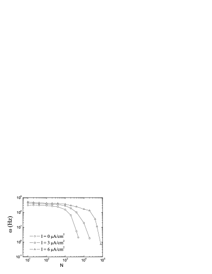
Figure 2: The mean firing frequency as a function of the channel cluster size $N$ for $I=0~{}\mu A/cm^{2}(\circ)$, $I=3~{}\mu A/cm^{2}(\square)$ and $I=6~{}\mu A/cm^{2}(\vartriangle)$. The data are obtained from spike trains of 2000 action potentials.

Voltage-gated ion channels are stochastic devices. The origin of channel noise is basically due to fluctuations of the fraction of open ion channels (thus the channel currents) around the corresponding mean values. The strength of the fluctuation is inversely proportional to the number of total ion channelsWhite1 ; Chow . Though average membrane current is at constant, as we will see, the variance of the $Na^{+}$ and $K^{+}$ currents cause remarkable effects on neuronal dynamics. In this work, we introduce channel cluster size $N$ ($N=N_{K}=N_{Na}/3$) as a measurement of channel noise level so that the correct proportion between $Na^{+}$ and $K^{+}$ channel densities is preserved. With increasing channel cluster size, the fluctuations of the fraction of open ion channels, thus the variance of the the corresponding channel currents decreases. For a large number of channels this noise becomes negligible (i.e., the deterministic case). The threshold constant current for deterministic HH neuron to generate consecutive action potentials is $I_{th}=6.26\mu A/cm^{2}$. However, due to the channel noise, the stochastic HH neurons can generate spiking activity with subthreshold input currentShangyou Zeng . Fig. 2 shows the mean firing frequency (defined in Sec. III) as a function of channel cluster size for different constant current. If the channel cluster size is small, the neuron fires action potentials with high frequency. As the channel cluster size increases, the mean firing frequency drops quickly, approaching the deterministic case that no firing activities occur with the same subthreshold input currents. With decreasing the input current, the firing frequency decreases. However, the firing activities will not vanish if the input current is decreased to zero. Thus, as have demonstrated, channel noise shifts the onset of firing behavior to lower values of input current $I$.

To explore the synchronization phenomena, we consider two stochastic HH neurons coupled by an electrical synaptic connection. The system is described by the following equations,

$$\frac{dV_{1}}{dt} = -\frac{N_{K_{1}}^{open}}{\tau_{K}N_{K_{1}}}(V_{1}-V_{K}^{rev})-\frac{N_{Na_{1}}^{open}}{\tau_{Na}N_{Na_{1}}}(V_{1}-V_{Na}^{rev})-\frac{1}{\tau_{L}}(V_{1}-V_{L})+\varepsilon(V_{1}-V_{2})+I_{1},$$ (7)

$$\frac{dV_{2}}{dt} = -\frac{N_{K_{2}}^{open}}{\tau_{K}N_{K_{2}}}(V_{2}-V_{K}^{rev})-\frac{N_{Na_{2}}^{open}}{\tau_{Na}N_{Na_{2}}}(V_{2}-V_{Na}^{rev})-\frac{1}{\tau_{L}}(V_{2}-V_{L})+\varepsilon(V_{2}-V_{1})+I_{2}.$$ (8)

Here $V_{1}$ and $V_{2}$ are the instantaneous membrane potentials of the two neurons and $\varepsilon$ is the diffusive coupling strength between the neurons. $N_{K_{1}}^{open}$, $N_{Na_{1}}^{open}$, $N_{K_{2}}^{open}$, $N_{Na_{2}}^{open}$ are the numbers of open $K^{+}$ and $Na^{+}$ channels of neuron $1$ and $2$, respectively ; $N_{K_{1}}$, $N_{Na_{1}}$, $N_{K_{2}}$, $N_{Na_{2}}$ are the numbers of total $K^{+}$ and $Na^{+}$ channels for neuron $1$ and $2$, respectively. $I_{1}$ and $I_{2}$ are two constant input currents which are set at $I_{1}=I_{2}=6\mu A/cm^{2}$. Here, $N_{1}$ and $N_{2}$ ($N_{i}=N_{K_{i}}=N_{Na_{i}}/3,\;i=1,2$) are the channel cluster sizes for each neuron.

The numerical integration of system mentioned above is carried out by using the Euler algorithm with a step size of $0.01$ms. And all simulations are working in Ito framework. The occurrences of action potentials are determined by upward crossings of the membrane potential at a certain detection threshold of 10mV if it has previously crossed the reset value of -50mV from below.

III frequency synchronization

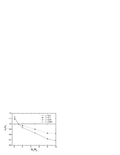
Figure 3: The winding number $\omega_{1}/\omega_{2}$ as a function of $N_{1}/N_{2}$ with $N_{2}=2\times 10^{2}$ and $\varepsilon=0.3$ ($\circ$), $\varepsilon=0.1$ ($\bullet$), $\varepsilon=0.01$ ($\ast$), $\varepsilon=0.001$ ($\square$).

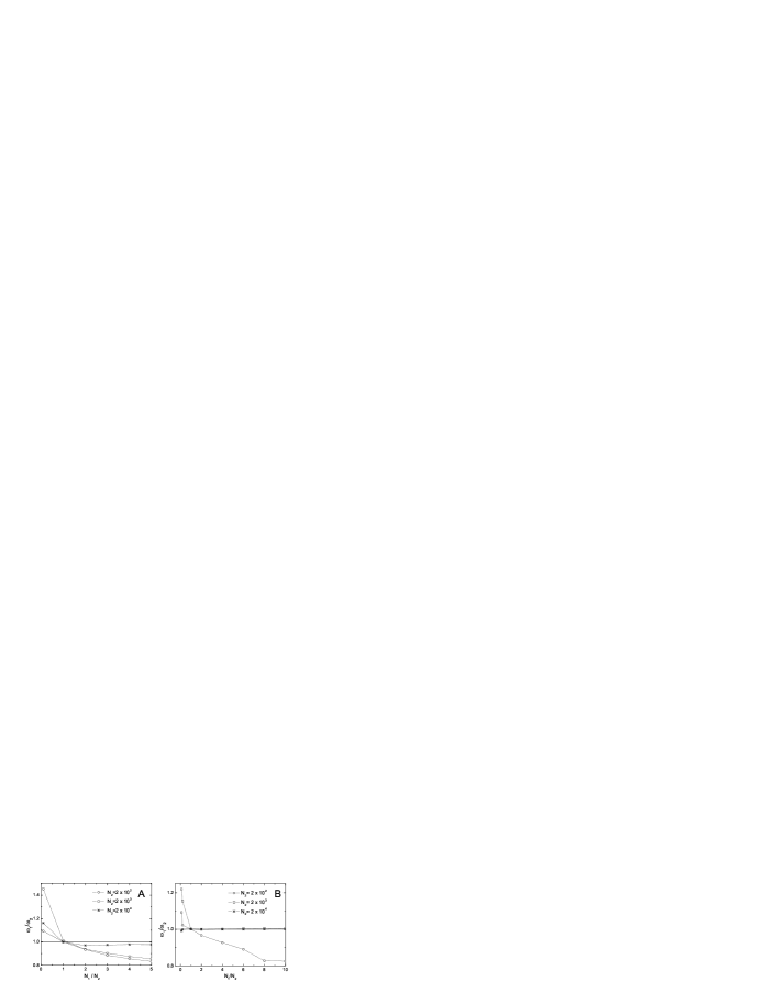
Figure 4: The winding number $\omega_{1}/\omega_{2}$ as a function of $N_{1}/N_{2}$ with $\varepsilon=0.01$ (A), $\varepsilon=0.1$ (B) and different $N_{2}$: $N_{2}=2\times 10^{2}$ ($\circ$), $N_{2}=2\times 10^{3}$ ($\square$) and $N_{2}=2\times 10^{4}$ ($\ast$).

From the above-mentioned system, we can get two point processes in the following form,

$$z(t)=\sum_{n=1}^{N}\delta(t-t_{n}).$$ (9)

Each one gives the spike sequence of a particular neuron. The mean spiking frequency of neuron $i$ ($i=1,2$) is defined as,

$$\omega_{i}=\lim_{N\ \rightarrow\infty}\frac{1}{N}\sum^{N}_{n=1}\frac{2\pi}{t_{n+1}-t_{n}},\;i=1,2.$$ (10)

Generally, synchronization means an adjustment of timescales of oscillations in systems due to their circumstances. In other words, oscillators can shift the timescales to make their ratio close to a rational number $n:m$, where $n$ and $m$ are integers. This phenomenon is usually referred to as $n:m$ frequency synchronization, and its suitable measure is the closeness of the ratio of $\omega_{1}/\omega_{2}$ to the chosen rational number $n:m$ Hauschild . In this paper we will discuss only $1:1$ synchronization. Note that the frequency locking discussed in this section is in a stochastic sense, and refers to the equivalence of the average frequencies rather than the instantaneous frequency. So it is not a sufficient condition for synchronization. However, since the firing rate of a neuron is often argued to carry information of the stimulus, studying of the frequency synchronization is especially meaningful in the context of rate coding scheme.

We investigated the shift of winding number $\omega_{1}/\omega_{2}$ along with both the variation of coupling strength and channel cluster size. When the coupling strength is small, as shown in Fig. 3, with the increasing of $N_{1}/N_{2}$ from $N_{1}/N_{2}<1$, the winding number will decrease from a value at which the two neurons are not synchronized. When two channel cluster sizes are the same ( $N_{1}/N_{2}=1$), both neuron will be frequency locked. Further increasing of $N_{1}/N_{2}$ will desynchronize them to a certain levels. Note that in the range of $N_{1}/N_{2}>1$, increasing the value of coupling strength tends to increase $\omega_{1}/\omega_{2}$, and the increasing is larger with larger coupling strength. In panel A of Fig. 4, it is seen clearly that though frequency synchronization can be achieved with arbitrary chosen value of $N_{2}$, the tuning is very critical, as a small variation of $N_{1}$ from $N_{2}$ leads to desynchronization. As has been described above, for a isolated neuron, its average firing rate decreases with increasing its channel cluster size (i.e., decreasing the channel noise intensity). Thus, at a given channel cluster size, the channel noise term is identical for the two neurons. In this case, their average firing rates would be the same, which means the two neurons are frequency locked.

However, if the coupling strength is increased to a rather large value (for example, $\varepsilon=0.3$ in Fig. 3), the coupling strength starts to take command of the frequency synchronization as the two neurons are able to be entrained in a wider range of channel cluster size (i.e., channel noise level). It is seen in panel B of Fig. 4 that neurons with larger value of $N_{2}$ is easier to get frequency entrained in a wider range with lower coupling strength. Even in the weak-coupling case, as shown in panel A of Fig. 4, large channel cluster sizes tend to enhance synchronization (make $\omega_{1}/\omega_{2}$ closer to 1). This implies that neurons with large channel cluster sizes (i.e., small channel noise level) are easier to adjust their timescales to make their firing rates close to each other. However, if the channel noises are too small, the neurons won’t fire spikes with subthreshold stimuli.

It is concluded that for identical, symmetrically coupled neurons, when the coupling strength is small, the channel cluster sizes at frequency synchronization must be the same, whereas the coupling strength only has a limited effect only when the channel cluster sizes of the two neurons are not same. However, when the coupling strength is rather large, the two neurons are able to achieve frequency synchronization with a greater range of channel cluster sizes. In this regime, though large channel noise degrade frequency synchronization, small channel noise intensities help to get the neurons frequency synchronized with subthreshold stimuli.

IV phase synchronization

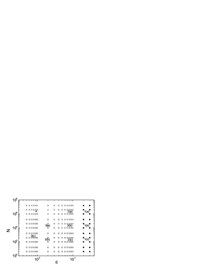
Figure 5: Synchronization diagram for the distribution of cyclic relative phase $P(\Phi)$. Region 1 correspond to state of monomodal distribution ($\bullet$), region 2 to bimodal distribution ($\circ$), region 3 to drifting evolution of $\Delta\phi$ ($\square$); region 4 to no firing area ($\times$). There are no lines plotted to separate the subregions in those regions because the distribution of $P(\Phi)$ changes in a continuous manner in those regions.

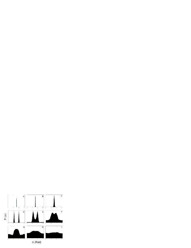
Figure 6: The distribution of the cyclic relative phase $P(\Phi)$ corresponding to some representative points of the synchronization diagram in Fig. 5. (A) $\varepsilon=0.3$, $N=2\times 10^{5}$; (B) $\varepsilon=0.3$, $N=2\times 10^{4}$; (C) $\varepsilon=0.3$, N$=2\times 10^{3}$; (D) $\varepsilon=0.08$, $N=2\times 10^{5}$; (E) $\varepsilon=0.08$, $N=2\times 10^{4}$; (F) $\varepsilon=0.08$, $N=2\times 10^{3}$; (G) $\varepsilon=0.02$, $N=2\times 10^{4}$; (H) $\varepsilon=0.02$, $N=2\times 10^{3}$; (I) $\varepsilon=0.004$, $N=2\times 10^{3}$. Each plane have different vertical scales.

Given a data set or some model dynamics there exists a variety of methods to define an instantaneous phase $\phi(t)$ of a signal or a dynamics Hanggi . However, for a stochastic system it is essential to assess the robustness of the phase definition with respect to noise. In many practical applications like neural spike sequence, it is useful to define an instantaneous phase $\phi(t)$ by linear interpolation,

$$\phi(t)=2\pi\frac{t-t_{n}}{t_{n+1}-t_{n}}+2\pi n\quad(t_{n}\leqslant t\leqslant{t_{n+1}}),$$ (11)

where $t_{n}$ is the time at which the neuron fires a spike. The instantaneous phase difference between them is then given by

$$\psi(t)=\phi_{1}(t)-\phi_{2}(t).$$ (12)

Phase synchronization is a weak form of synchronization in which there is a bounded phase difference of two signals. Usually, the relative phase can vary from $-\infty$ to $+\infty$ in stochastic system if the coupling is weak and/or the noise level is high. However, if we increase coupling strength and adjust noise to a low level, the relative phase will fluctuate around some constant values. Sometimes, noise would induce a phase slip where the relative phase changes abruptly by $\pm 2\pi$. Thus, it is useful to define the phase locking condition in a statistical sense by the cyclic relative phase kurth

$$\Phi=\psi(mod2\pi).$$ (13)

A dominant peak of the distribution of this cyclic relative phase $P(\Phi)$ reflects the existence of a preferred relative phase for the firing of both neurons. When this preferred phase is zero we speak of phase synchronization in a statistic sense. We speak of out-of-phase synchronization when the distribution $P(\Phi)$ peaks around a nonzero value of $\Phi$. Especially if the nonzero value is $\pi$, we call it antiphase synchronization Hanggi ; Casado2 .

IV.1 phase synchronization of identical neurons

In this section, we study phase synchronization of two identical neurons ($N_{1}=N_{2}=N$). In Fig. 5, we present the synchronization diagram in terms of the coupling strength $\varepsilon$ and channel cluster size $N$. A different form of the distribution $P(\Phi)$, which is plotted in Fig. 6, characterizes each region in it. The corresponding temporal evolution of the relative phase is illustrated in Fig. 7. We will give a detailed description of each region in the following part.

In region 1, the distribution shows a monomodal character as plotted in panel A, B, C of Fig. 6. In this region, when both $\varepsilon$ and $N$ are very large, the distribution of $P(\Phi)$ is a narrow peak on $\pi$. Thus we can speak of antiphase synchronization for a statistic out-of-phase locking is achieved. With the decreasing of $N$, the peak is still on $\pi$ but becomes broader(see the change of peaks in $A\rightarrow B\rightarrow C$ ). This suggests that in the case of large coupling strength, large channel cluster size (i.e., small channel noise) allow the statistical antiphase synchronization to approach full antiphase synchronization appearing in deterministic systems. As can be seen in Fig. 5, there is a minimal value of the coupling strength $\varepsilon_{0}$ for which the antiphase locking becomes stable in a statistical sense. This minimal coupling strength $\varepsilon_{0}$ ($\approx$ 0.115) is independent of the channel cluster size. To show the effect of channel noise on antiphase synchronization, we demonstrated the temporal evolution of relative phase in this situation in panel A and B of Fig. 7. Obviously, decreasing channel cluster sizes will lead to larger fluctuation of the relative phase due to channel noise, thus give distribution of $P(\Phi)$ a broader peak, but it does not destruct antiphase synchronization.

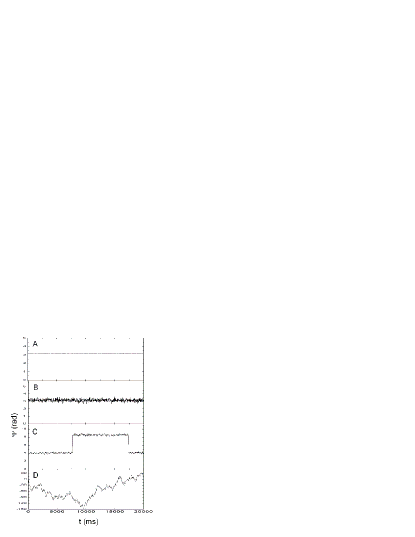
Figure 7: Temporal evolution of the relative phase (A) $\varepsilon=0.3$, $N=2\times 10^{5}$; (B) $\varepsilon=0.3$, $N=2\times 10^{3}$; (C) $\varepsilon=0.08$, $N=10^{4}$; (D) $\varepsilon=0.02$, $N=2\times 10^{3}$.

Region 2 marked by open circles corresponds to the bimodal distribution of $P(\Phi)$, as shown in panel D, E and F of Fig. 6. In this region, when $\varepsilon$ and $N$ are large [2(a)], the two peaks of the distribution are well spaced from each other. To uncover the underlying mechanism of this bimodal distribution, we investigated the temporal evolution of relative phase in this situation. As we observed in panel C of Fig. 7, $\psi(t)$ will fluctuates successively around one of a pair of symmetric values for a long period then switch suddenly to the other one. This fact clearly reflects the two-state character of the phase dynamics. We argue that this two-state dynamics is the result of a compromise between coupling and noise. The existence of a two-state dynamics suggests the possibility of inducing a kind of stochastic resonant behavior by coupling the relative phase to the action of an external periodic forcing Casado2 . Again, if we decrease $N$ to enter 2(b) area, the two peaks will be broader, and gradually overlapped and have small wings. The overlapping means that the bimodal distribution becomes unstable. The wings implies that preferred relative phase for the firing of both neurons does not prefer to some certain values anymore, thus the synchronization becomes weak. If we further decrease $N$ to enter 2(c) area, we find that the two peaks move closer and then merge but still have a maxima around $\pi$ (see panel F of Fig. 6.)

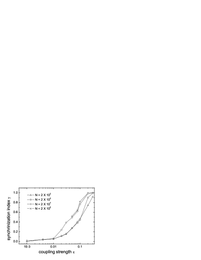
Figure 8: Synchronization indices for two identical neurons versus coupling strength with various ion channel cluster sizes $N$.

Actually, the phase-locking phenomena in noise-free neural systems have been well studied through effective coupling analysisSeon Hee Park 1 ; Seung ; Seon Hee Park . S. K. Han and Kuramoto had demonstrated that diffusive interaction will dephase interacting oscillators and may stabilize them at a phase difference given by the corresponding stable fixed point according to the initial condition (see detail in Ref. Seung ). In our case, those stable fixed points are stochastic variables with single peaks distribution alike the peaks demonstrated in Fig. 6. In region 1, there is only one stable fixed point distributed around $\pi$ and will become broader if the noise intensity is increased. In region 2, the system has two stable fixed points. The system will be stabilized at one point according to the initial condition, then the channel noise occasionally change the initial condition and stabilized the system at the other one. If the channel cluster size $N$ is extremely large, though there are still two stable fixed point, the channel noise is too weak to change the initial condition frequently, and only one of the two peaks can be observed with certain recording time interval(not shown). As $N$ decreases, the channel noise becomes larger, giving broader distributions of the two stable fixed points and more frequent switches between them. It is the broader distributions of the two stable fixed points that leads the overlapping of the two peaks in this area.

In region 3, we find the bimodal distribution of $P(\Phi)$ mentioned before disappears and the single peak distribution appears again with large wings. Panel G of Fig. 6 shows a representative cyclic relative phase distribution corresponding to the 3(a) area, which is characterized by a peak around $\pi$ and another smaller one around $0$. If we decreasing the coupling strength to enter 3(b) area from 2(c) area, the central peaks will decrease in height [panel H ] and eventually disappear [3(c) area, panel I]. In 3(c) area, the relative phase will drift unboundedly and $P(\Phi)$ ceases to be useful (see panel D of Fig. 7). When the coupling strengths is very weak, the system at hand can be considered as two uncoupled neurons which fire independently due to ion channel noise. Thus their relative phase can be at any arbitrary value (as show in panel D of Fig. 7), and gives relative phase a smooth distribution.

Region 4 in Fig. 5 is the silent state in which both neurons cannot fire spikes but only perform low amplitude fluctuations around its resting potentials under the combining effects of coupling and channel noise.

Next, we characterize those peaks with synchronization indices which are defined as

$$\gamma^{2}=\langle cos\Phi(t)\rangle^{2}+\langle sin\Phi(t)\rangle^{2},$$ (14)

where $\langle...\rangle$ denotes temporal averaging. The index $\gamma$ assumes values between 0 (no synchronization) and 1 (perfect phase locking)Hauschild .

Fig. 8 quantitatively demonstrated the synchronization of two identical neurons under the effect of both coupling strength and channel noise. When coupling strength is small, the two neurons show almost no synchronization [$\gamma\approx 0$, corresponding to 3(c) area of Fig. 5] or silent state when $N$ is large(incomplete lines, corresponding to region 4 of Fig. 5). The synchronization index $\gamma$ is not sensitive to the change of channel cluster size $N$ in small coupling strength region. As the coupling strength increases the degree of synchrony of the two neurons increases. The maximal synchrony appears at $\gamma\approx 1$ (corresponding to region 1 of Fig. 5). Note that when channel cluster sizes are large, as shown in Fig. 5, there exists a step-like transition (a threshold) to perfect synchronization. The threshold is around about $\varepsilon=0.04$ when $N=2\times 10^{5}$. However, it disappears when cluster sizes decrease, and the transition becomes a graded type. It implies that channel noise can ’soft’ the threshold to give a wider range of synchronization degree.

IV.2 phase synchronization of nonidentical neurons

Figure 9: The distribution of the cyclic relative phase $P(\Phi)$ for nonidentical neurons. (A)$\varepsilon=0.2,N_{1}=2\times 10^{2}$, $N_{2}=2\times 10^{3}$; (B)$\varepsilon=0.08,N_{1}=1\times 10^{5}$, $N_{2}=2\times 10^{4}$; (C)$\varepsilon=0.03,N_{1}=2\times 10^{2}$, $N_{2}=2\times 10^{3}$. Each plane have different vertical scales.

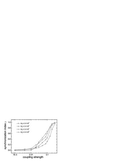
Figure 10: Synchronization indices for two nonidentical neurons versus coupling strength with channel cluster size of the first neuron $N_{2}=2\times 10^{3}$.

Actually, neurons in nature are not identical. The nonidentity can be achieved in numerical simulation by mismatching neuronal parameters (the leakage conductance $g_{l}$, for example) Changsong Zhou . Here, we introduce a mismatch into the channel cluster sizes of the two neurons (i.e., $N_{1}\neq N_{2}$). With this parameter heterogeneity, the neuron with smaller channel cluster size, due to its larger channel noise, is easier to be excited by subthreshold stimuli and has larger firing rate than another one.

In the case of two nonidentical neurons, the above mentioned cyclic relative phase distributions are still tenable and the perfect phase synchronization can also be achieved (see Fig. 10). However, there are three exceptions. First, because the symmetry of the distribution $P(\Phi)$ is dependent on the symmetry of the system, for nonidentical neurons the distribution of the cyclic relative phase is asymmetric (see Fig. 9). This fact was also confirmed by applying different tonic subthreshold currents to two neurons to make the system asymmetric Casado2 . Second, as mentioned before, the two weakly coupled identical neurons with large channel cluster sizes are unable to fire spikes under a subthreshold stimulus (see the plot of $N=2\times 10^{5}$ in Fig. 8). However, when a neuron with large channel cluster size coupled with a small one which could be excited by subthreshold stimulus due to channel noise, the large one is excited by the small one through coupling. As shown in Fig. 10, comparing with identical situation, the neuron can be excited when $N=2\times 10^{5}$ and $\varepsilon$ is rather small. It is also seen that in the weak coupling region, the identical neurons exhibit higher degree of synchronization than the nonidentical ones. Whereas in the strong coupling region, when a neuron is coupled to another one which has larger $N$, they exhibit higher degree of synchronization. This is consistent with the frequency synchronization case where identical neuron is frequency locked even coupling is weak, but nonidentical neuron can also be synchronized if the coupling is strong, and neurons with large channel clusters are easier to get synchronized.

V CONCLUSION

In conclusion, the frequency and phase synchronization of two coupled stochastic Hodgkin-Huxley neurons are studied by varying coupling strength and channel cluster sizes. The two neuron is coupled via a gap junction because the gap-junctional (diffusive) coupling can generate rich dynamical behavior Sherman . What’s more, with this simple coupling, we could emphasized on the effects of channel noise and ignore the inessential details of complex synaptic process. Our studies show that when the coupling is weak, the cluster sizes of the two neurons must be the same to achieve frequency synchronization, and the synchronization region is very narrow. However, when coupling is strong, the two neurons can be frequency entrained in a wide region. For two identical neurons, a state of statistical antiphase synchronization is reached in the strong coupling region if the cluster size is large enough. In this state, the relative phase between two spike trains would be around $\pi$. As the coupling strength and channel cluster size are reduced, the phase-locking condition is lost and a rather complex behavior would appear. This complex behavior, as we have argued, is the result of a compromise between coupling strength and channel noise. We use synchronization indices to characterize the transitions to synchronization, and find that there exit a threshold to synchronization. When channel cluster sizes are small, channel noise can ’soft’ this threshold to present synchronization at a wider range. For two nonidentical neurons, the distribution of the cyclic relative phase is asymmetric and the silent state in identical situation disappears. This, as we have pointed out, is due to asymmetric of the system and spontaneous firing induced by channel noise.

It is helpful that our study is important for the understanding of coupled stochastic systems and possible applications especially in neuroscience where the synchronization activity could be tuned through the control of the channel noise via channel blocking. By applying channel cluster size control to real neural systems one should be able to influence neural synchrony. Further work should focus on more sophisticated models and on coupling more than two neurons.

References

- (1) A. Pikovsky, M. Rosenblum, and J. Kurths, Synchronization: a Universal Concept in Nonlinear Science. (UK, Cambridge, 2001).
- (2) C. M. Gray, P. Koning, A. K. Engel, and W. Singer, Nature 338, (1989) 334.
- (3) R. C. Elson, A. I. Stlverston, and R. Huerta, Phys. Rev. Lett. 81, (1998) 5692.
- (4) R. D. Pinto, P. Varona, and A. R. Volkovskii, Phys. Rev. E 62, (2000) 2644.
- (5) Q. Li, Y. Chen, and Y. H. Wang, Phys. Rev. E 65, (2002) 041916.
- (6) R. Fitzgerald, Physics Today, March edition, (1999) 17.
- (7) G. Uchida, M. Fukuda, and M. Tanifuji, Phys. Rev. E 73, (2006) 031910.
- (8) A. S. Pikovsky, Phys. Lett. A 165, (1992) 33.
- (9) A. Maritan and J.R. Banavar, Phys. Rev. Lett. 72, (1994) 1451.
- (10) A. S.Pikovsky, Phys. Rev. Lett. 73, (1994) 2931.
- (11) C. S. Zhou and C. H. Lai, Phys. Rev. E 58, (1998) 5188.
- (12) H. Herzel and J.freund, Phys. Rev. E 52, (1995) 3238.
- (13) Y. Q. Wang, D. T. Chik, and Z. D. Wang, Phys. Rev. E 61, (2000) 740.
- (14) I. Z. Kiss, Y. Zhai, and J. L. Hudson, Chaos 13, (2003) 267.
- (15) C. S. Zhou and J. Kurths, Chaos 13, (2003) 401.
- (16) B. Hille, Ionic channels of excitable membranes, (Sunderland, MA, Sinauer Associates, 2001).
- (17) J. A. White, J. T. Rubinstein, and A. R. Kay, Trends. Neurosci. 23, (2000) 131.
- (18) E. Schneidman, B. Freedman, and I. Segev, Neural Comput. 10, (1998) 1679.
- (19) C. C. Chow and J. A. White, Biophys. J. 71, (1996) 3013.
- (20) J. M. Casado, Phys. Lett. A 310, (2003) 400.
- (21) J. M. Casado and J. P. Baltanas, Phys. Rev. E 68, (2003) 061917.
- (22) S. Y. Zeng and P. Jung, Phys. Rev. E 70, (2004) 011903.
- (23) G. Schmid, I. Goychuk, and P. Hänggi, Phys. Biol. 1, (2004) 61.
- (24) A. L. Hodgkin and A. F. Huxley, J. Physiol. 117, (1952) 500.
- (25) B. Hauschildt, N. B. Janson, and A. Balanov, Phys. Rev. E 74, (2006) 051906.
- (26) P. Dayan and L. F. Abbott, Theoretical neuroscience: computational and mathematical modeling of neural systems, (USA, MIT press, 2001).
- (27) J. A. Freund, L. Schimansky-Geier, and P. Hänggi, Chaos 13, (2003) 225.
- (28) S. H. Park, S. W. Kim, H. B. Pyo, and S. Lee, Phys. Rev. E 60, (1999) 2177.
- (29) S. K. Han, C. Kurrer, and Y. Kuramoto, Phys. Rev. Lett. 75, (1995) 3190.
- (30) S. H. Park, S. K. Han, and S. W. Kim, ETRI J. 18, (1996) 161.
- (31) A. Sherman and J. Rinzel, Proc. Natl. Acad. Sci.(USA) 89, (1992) 2471.