Extinction Rates for Fluctuation-Induced Metastabilities : A Real-Space WKB Approach

Abstract

The extinction of a single species due to demographic stochasticity is analyzed. The discrete nature of the individual agents and the Poissonian noise related to the birth-death processes result in local extinction of a metastable population, as the system hits the absorbing state. The Fokker-Planck formulation of that problem fails to capture the statistics of large deviations from the metastable state, while approximations appropriate close to the absorbing state become, in general, invalid as the population becomes large. To connect these two regimes, a master equation based on a real space WKB method is presented, and is shown to yield an excellent approximation for the decay rate and the extreme events statistics all the way down to the absorbing state. The details of the underlying microscopic process, smeared out in a mean field treatment, are shown to be crucial for an exact determination of the extinction exponent. This general scheme is shown to reproduce the known results in the field, to yield new corollaries and to fit quite precisely the numerical solutions. Moreover it allows for systematic improvement via a series expansion where the small parameter is the inverse of the number of individuals in the metastable state.

Local extinction due to demographic stochasticity is a key issue in the analysis of persistence and viability of small populations.1 ; 2 In particular, it allows ecologists to identify endangered species and to specify conservation policies, it dictates the appearance and disappearance of favored and neutral genetic mutations 5 and is of importance in the determination of the critical population size needed to support an epidemic.3 As in most cases of rare and extreme events the important quantities to be measured and compared with the theory are the expected extinction time of the populations,1 and the probability distribution close to the absorbing state. Technically, however, the effect of demographic stochastisity has traditionally been taken into account using some version of a Fokker-Planck equation, where the ”diffusion coefficient” is a function of the population size.1

Recently, much interest has been focussed on the calculation of extinction rates for systems whose macroscopic dynamics exhibits a stable state which is nevertheless only metastable due to rare fluctuations which can drive the system to extinction.ek ; b ; c ; am In particular, it has been realized that in general the Fokker-Planck (FP) expansion about the (meta-)stable state is incapable of predicting the extinction rate. This is due to the fact that the Fokker-Planck expansion is only valid for up to $O(N^{2/3})$ fluctuations to the large, $O(N)$, number of particles in the metastable state. The FP approximation fails to correctly describe the very large fluctuations necessary to reach the absorbing state of zero particles. The FP treatment also smears out the microscopic differences between processes as it reflects a local analysis close to the metastable fixed point. In order to get the correct statistics for rare and extreme events one should base the estimate on the exact Master equation that describes the stochastic process, and to employ the method of extreme statistics, or more simply put, the WKB approximation, to solve the relevant master equation.

Elgart and Kamenev ek made an interesting observation in this context: using the Peliti-Doi pd ; cardy technique to map the exact master equation into a ”quantum mechanical” problem (Schroedinger-like equation in imaginary time with second quantized Hamiltonian) they were able to identify the classical trajectory that connects the metastable fixed point and the absorbing state. This identification allows them to calculate the classical (”geometrical optics”) action along this trajectory, a first approximation to the extinction time. Assaf and Meersonam then suggest a general spectral method to improve beyond the Elgart-Kamenev results, employing the generating function formalism and using the Sturm-Liouville theory of linear differential operators.

In this paper, we will present a general scheme to deal with the local extinction problem, based on the time-independent ”real space” WKB approximation (unlike Refs. ek ; am who used a time-dependent momentum space presentation). The method presented is easy to use, its intuitive meaning is transparent, and its range of applicability covers, essentially, any single species problem.

This paper will be organized as follows: In the next section we exemplify the technique for what is perhaps the archetypical problem in this class, a logistic birth-death process of a single species. Beside its importance, the solution of this example demands the use of all the components of the technique - a Fokker-Planck solution applicable close to the metastable fixed point, small $n$ approximation close to the absorbing state and a WKB solution that encompasses the FP regime and connects to the small $n$ region. This model, thus, serves also as a nice pedagogical introduction. The third section deals with a similar birth death process, but when the number of offsprings at each birth event is two, as in the case of domain walls in magnetic systems. Here, a series of mathematical ”miracles” occur, which allow for a simple calculation of the extinction rate (for the case of an initial even number of particles) without recourse to the WKB method. In the fourth section the effect of a single agent death term is incorporated, and in the last section the marginal case of neutral mutation is analyzed. We then conclude with a summary and some final observations.

I Stochasticity, logistic growth and extinction

In this section we study the stochastic dynamics of a combination of two fundamental processes: particles giving birth to new particles at rate $\alpha$; and pair annihilation at rate $\beta$. In that case the average number of particles is about $\alpha/\beta$. The full ”physical optics” solution for both the probability distribution, $P_{n}$, of the metastable state and the extinction rate, in the limit where $\beta\ll\alpha$ is given, based on a WKB approximation for the exact master equation. We confirm our calculations by comparison to a direct numerical solution of the master equation.

The microscopic rules that govern this process are:

$$P \stackrel{{\scriptstyle\alpha}}{{\to}} 2P$$

$$P+P \stackrel{{\scriptstyle\beta}}{{\to}} 0$$ (1)

The exact master equation for $P_{n}$, the probability of having $n$ particles, is

$$\dot{P}_{n}=\alpha\left[-nP_{n}+(n-1)P_{n-1}\right]+\frac{\beta}{2}\left[-n(n-1)P_{n}+(n+2)(n+1)P_{n+2}\right]$$ (2)

At the mean-field level the process is described by the reaction equation,

$$\dot{n}=\alpha n-\beta n(n-1)$$ (3)

which has the stable solution $n=\alpha/\beta+1$. Technically, this expression may be derived from the exact master equation (2) by calculating the time derivative of the average population $\dot{\langle n\rangle}\equiv\sum n\dot{P_{n}}$ and using the approximation $\langle n^{2}\rangle=\langle n\rangle^{2}$. The stable solution becomes metastable due to the effect of stochastisity (in particular, all particles may annihilate each other and the system will be stuck in the absorbing state $P_{0}=1$). Our aim is to calculate the typical time of this extinction event.

Since that stochastic process has no memory (a Markov process) it may be described by a transition matrix that specify the rates to pass from one microscopic configuration to the other. Clearly, the absorbing state $\{P_{0}=1,\ P_{n}=0\ \forall n\neq 0\}$ is an eigenvector of that matrix with an eigenvalue 0. All other eigenstates admit negative eigenvalues, and we denote the absolute value of the highest of these eigenvalues as $\Gamma$. The corresponding eigenvector is the stochastic metastable state, so our mission is to calculate $\Gamma$. Our main interest is in the case $\alpha/\beta\gg 1$ so that the typical number of particles is large. This implies that the probability to reach the absorbing state is, as we will calculate, exponentially small.

The metastability of the system implies that at long times the $P_{n}$ decay exponentially as $e^{-\Gamma t}$. Thus we need to solve the master equation with the left-hand side replace by $-\Gamma P_{n}$. However, since $\Gamma$ is exponentially small, we can drop this term altogether. Technically this implies that we only have to solve for a steady state vector rather than doing time dependent semiclassical analysis which is much more complicated.

I.1 Fokker-Planck equation and its limitations

The standard approach for solving the now time-independent master equation is to transform it into a Fokker-Planck (FP) equation 2 . The nominal prescription for doing this is to expand $P_{n\pm 1}$, etc. in a Taylor series, dropping terms involving more than two derivative. However, phrasing the problem this way does not explain why, or more specifically, when this procedure is justified; moreover, the emerging equation is not unique - the same expansion may be done for $nP_{n}$, for example, yielding different equation. The real justification underlying the Fokker-Planck approximation is that, for small $\beta/\alpha$, $P_{n}$ is a smooth function of the $O(1)$ variable

$$y\equiv\left(\frac{\beta}{\alpha}\right)^{1/2}\left(n-\frac{\alpha}{\beta}\right)$$ (4)

Then, $P_{n\pm 1}$ is equal to $P(y\pm\sqrt{\beta/\alpha})$ and so may be expanded formally with regard to the small parameter $\beta/\alpha$. The resulting series may be written as:

$$\alpha\left[\hat{{\cal L}}_{0}P(y)+\sqrt{\frac{\beta}{\alpha}}\ \hat{{\cal L}}_{1}P(y)+{\cal O}\left(\frac{\beta}{\alpha}\right)+...\right]=0$$ (5)

where

$$\hat{{\cal L}}_{0}=\left(\frac{d}{dy}(yP)+\frac{3}{2}\frac{d^{2}}{dy^{2}}P\right)$$ (6)

and

$$\hat{{\cal L}}_{1}=\frac{1}{2}\left(P^{\prime\prime\prime}+5yP^{\prime\prime}+8P^{\prime}+4yP+2y^{2}P\right)$$ (7)

This perturbative expansion is justified (at least in the sense of asymptotic series) if, expanding $P(y)=P_{0}(y)+\sqrt{\beta}{\alpha}P_{1}(y)+\ldots$, the correction term $\sqrt{\beta/\alpha}P_{1}(y)\ll P_{0}(y)$. Plugging this series into (5) and collecting terms order by order one finds that

$$P_{0}(y)=Ce^{-y^{2}/3}=Ce^{-\beta(n-\alpha/\beta)^{2}/3\alpha}.$$ (8)

Then, looking at the equation for $P_{1}$

$$\hat{{\cal L}}_{0}P_{1}(y)=-\sqrt{\frac{\beta}{\alpha}}\ \hat{{\cal L}}_{1}P_{0}(y),$$ (9)

one is able to identify that the leading correction is proportional to $y^{3}\sqrt{\beta/\alpha}P_{0}(y)$. Thus the the FP equation is only valid up to $(n-\alpha/\beta)\sim(\alpha/\beta)^{2/3}$, as mentioned above. This limit on the FP reliability is clearly demonstrated in Figure 1, where for a metastable population of 100 individuals the FP solution is a good approximation to the exact probability distribution between 100 and 70.

To find the decay rate, however, we need to have a solution valid down to $n=1$, and the FP solution does not suffice. One can try to consider the low $n$ limit of the master equation.

I.2 Probability distribution close to extinction

In the vicinity of the absorbing state one may use a simplified form of the master equation, exploiting the fact that $P_{n}$ is a rapidly growing function of $n$. Then, $P_{n}\ll P_{n+2}$ and $P_{n-1}\ll P_{n}$, yielding the simplified recursion relation:

$$P_{n+2}=\left(\frac{2\alpha}{\beta}\right)\frac{n}{(n+2)(n+1)}P_{n}$$ (10)

This approximate recursion relation leaves the even and odd $n$’s decoupled, and has the solution

$$P_{2k} = \left(\frac{4\alpha}{\beta}\right)^{k-1}\frac{2(k-1)!}{(2k)!}P_{2}$$

$$P_{2k+1} = \left(\frac{\alpha}{\beta}\right)^{k}\frac{1}{(2k+1)k!}P_{1}$$ (11)

with $P_{1}$, $P_{2}$ arbitrary. Examining Eq. (10), we see that if $P_{1}\ll P_{2}$, then as long as $n\ll\alpha/\beta$, our assumption leading to the approximate recursion relation is valid. It is also clear that the rapid rise of the $P_{n}$’s slows as $n$ increases, with the $P_{n}$’s reaching a maximum at $n=2\alpha/\beta$. Clearly, however, the maximum probability state is at $n\approx\alpha/\beta$, so the recursion relation must fail before the bulk regime. In fact, our recursion relation works up to $\beta n/\alpha\ll 1$ whereas the FP solution only works when $\beta n/\alpha\approx 1$. There is no way to directly connect these two regimes. This is seen clearly in Fig. 1, where the recursion relation and FP solutions are shown for the case $\beta/\alpha=0.01$. The resolution to this problem lies in the WKB method, which will allow us to connect the recursion relation results to the FP regime.

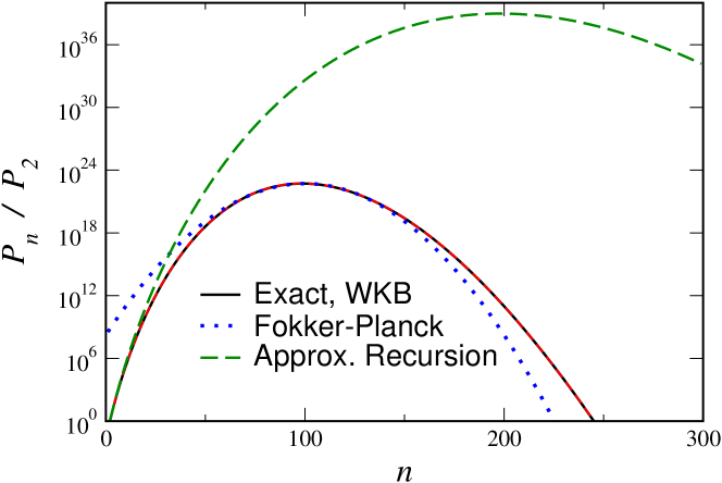
Figure 1: Probability distribution $P_{n}/P_{2}$ for $\beta=0.01$, $\alpha=1$, for the basic model, Eq. (1), together with the WKB approximation, Eq. (30), together with (16), (29), and (32); the FP approximation, Eq. (33); and the low/intermediate-$n$ result, Eq. (11). Note that on the scale of the figure, the WKB approximation is indistinguishable from the exact result.

I.3 WKB approximation and the extinction rate - the leading term

To do WKB for our difference equation,bender we write $P_{n}=e^{S_{n}}$, where $S_{n}$ is assumed to be a smooth function of $n$, so that $S_{n\pm 1}\approx S_{n}\pm S^{\prime}_{n}$. Since we already know (from the FP treatment) that the probability profile in the bulk is a Gaussian with width proportional to the square root of the metastable population, the quality of this approximation is controlled. Writing $\Lambda_{n}\equiv e^{S_{n}^{\prime}}$, we have, assuming $n\gg 1$,

$$0=\alpha\left(-n+\frac{n}{\Lambda_{n}}\right)+\frac{\beta}{2}\left(-n^{2}+n^{2}\Lambda_{n}^{2}\right)$$ (12)

or, simplifying,

$$0 = \beta n\Lambda_{n}^{3}-(2\alpha+\beta n)\Lambda_{n}+2\alpha$$ (13)

$$= (\Lambda_{n}-1)(\beta n\Lambda_{n}^{2}+\beta n\Lambda_{n}-2\alpha)$$

where we have factored out the trivial $\Lambda_{n}=1$ root which is a result of conservation of probability. The other two roots for $\Lambda$ are

$$\Lambda_{n}=-\frac{1}{2}\pm\frac{\sqrt{1+\frac{8\alpha}{\beta n}}}{2}\ ,$$ (14)

of which the larger, positive, one is relevant for us, since we want $P_{n}$ to be an increasing function. This implies that

$$S^{\prime}_{n}=\ln\left(\frac{\sqrt{1+\frac{8\alpha}{\beta n}}-1}{2}\right)$$ (15)

Integrating, we find that

$$S_{n}=S_{0}+n\ln\left(\sqrt{1+\frac{8\alpha}{\beta n}}-1\right)+\frac{1}{2}n\sqrt{1+\frac{8\alpha}{\beta n}}-\frac{2\alpha}{\beta}\ln\left(\frac{\beta n}{4\alpha}+1+\frac{\beta n}{4\alpha}\sqrt{1+\frac{8\alpha}{\beta n}}\right)-n\ln(2)+\frac{1}{2}n$$ (16)

The first important point to notice is that $\alpha/(\beta n)$ extrapolates, in the interesting region, from $\infty$ as $n\to 0$ to unity, where $n\to\alpha/\beta$. In the first case $S^{\prime}$ scales logarithmically with $\alpha/(\beta n)$, hence $S_{n}$ is proportional to $\alpha/(\beta n)$ and is large. In the second regime $S^{\prime}$ is almost constant and $S_{n}$ scale with $n$ which is also, in that case, large. Thus all the way to extinction $S_{n}$ is large, as expected. Evaluating $\Delta S\equiv S_{\alpha/\beta}-S_{0}$, one obtains

$$\Delta S=\frac{2\alpha}{\beta}\left(1-\ln(2)\right)$$ (17)

in agreement with the result of Elgart and Kamenev.ek

We can make the connection to the formalism presented in ek even more explicit, if we express the relations in terms of $n(\Lambda)$ as opposed to $\Lambda_{n}$. From Eq. (13),

$$n(\Lambda)=\frac{2\alpha}{\beta\Lambda(\Lambda+1)}$$ (18)

thus

$$\Delta S = \int_{0}^{\alpha/\beta}\ln(\Lambda_{n})dn$$ (19)

$$= -\int_{1}^{\infty}\ln(\Lambda)\frac{dn}{d\Lambda}d\Lambda$$

$$= -\ln(\Lambda)n(\Lambda)|_{1}^{\infty}+\int_{1}^{\infty}\frac{n(\Lambda)}{\Lambda}d\Lambda$$

$$= \int_{1}^{\infty}\frac{n(\Lambda)}{\Lambda}d\Lambda.$$

If we now introduce the ”momentum” $p\equiv 1/\Lambda$ and the ”coordinate” $q\equiv n\Lambda$, the expression for $\Delta S$ may be rewritten as

$$\Delta S=\int_{0}^{1}qdp$$ (20)

where

$$q(p)=\frac{2\alpha}{\beta}\frac{p}{1+p}$$ (21)

precisely reproducing Elgart-Kamenev equations for the action and the semiclassical escape path. The physical meaning of the ”momentum” $p$ is now clarified: it is the inverse of the geometrical growth rate of the quasistatic probability distribution.

We now need to confirm that there exists an overlap region between the WKB solution and the $n\ll\alpha/\beta$ recursion regime. For $n\ll\alpha/\beta$ our WKB solution for $S_{n}$ may be approximated by,

$$S_{n}\approx S_{0}+\frac{1}{2}n\left(1+\ln\left(\frac{2\alpha}{\beta n}\right)\right)$$ (22)

To compare this with the recursion relation results, Eq. (11), in the limit $n\gg 1$:

$$\ln(P_{n}^{\it even}) \approx \frac{1}{2}n\left(1+\ln\left(\frac{2\alpha}{\beta n}\right)\right)+\frac{3}{2}\ln(2)-\ln\left(\frac{4\alpha n}{\beta}\right)+\ln(P_{2})$$

$$\ln(P_{n}^{\it odd}) \approx \frac{1}{2}n\left(1+\ln\left(\frac{2\alpha}{\beta n}\right)\right)-\frac{1}{2}\ln\left(\frac{2\pi\alpha n^{2}}{\beta}\right)+\ln(P_{1})$$ (23)

Indeed, the leading order asymptotics agrees.

In the other extreme our WKB result coincides with the FP treatment. Expanding the WKB solution for small $y\equiv\sqrt{\beta/\alpha}(n-\alpha/\beta)$ yields

$$\ln(S_{n})=\ln(\Delta S-y^{2}/3)$$ (24)

indeed reproducing the FP solution.

I.4 WKB approximation and the extinction rate - first order corrections

The explicit real space, time-independent WKB analysis allows one to go beyond the Elgart-Kamenev ”geometrical optics” results and to obtain the leading corrections. In the previous subsection the generic substitution $P_{n}=\exp(S_{n})$ was implemented and is justified ex post facto by the fact that $S_{n}$ turns out to be ${\cal O}(\alpha/\beta)>>1$. To proceed let us assume that

$$P_{n}=\exp(S_{0}(n)+S_{1}(n)+S_{2}(n)+...)$$ (25)

where $S_{0}(n)$ is the leading order $S_{n}$ found above and $S_{m}(n)$ is assumed to be $O((\beta/\alpha)^{m-1})$. Beginning with the growth part of the master equation $T_{\alpha}\equiv\alpha[-nP_{n}+(n-1)P_{n-1}]$, plugging in Eq. (25) and expanding the small (${\cal O}(\beta/\alpha)$) terms in the exponent one has (note that any derivative adds a $(\beta/\alpha)$ factor):

$$T_{\alpha} = \alpha e^{S_{0}(n)+S_{1}(n)+S_{2}(n)}\left(-n+(n-1)e^{-S_{0}^{{}^{\prime}}(n)}\left[1+\frac{1}{2}S_{0}^{{}^{\prime\prime}}-S_{1}^{{}^{\prime}}\right]\right)$$ (26)

$$= \alpha ne^{S_{0}+S_{1}+S_{2}}\left[\left(-1+\frac{1}{\Lambda_{n}}\right)+\frac{1}{\Lambda_{n}}\left(\frac{S_{0}^{{}^{\prime\prime}}}{2}-S^{\prime}-\frac{1}{n}\right)\right]$$

While the first, ${\cal O}(1)$, term in the bracket was used to determine $\Lambda$, the second ${\cal O}(\beta/\alpha)$ term will be used here in order to find the function $S_{1}$. Repeating that procedure and collecting the leading corrections from the annihilation part of the Master equation one finds,

$$0=\frac{\alpha}{\Lambda_{n}}\left(-S_{1}^{\prime}+\frac{S_{0}^{\prime\prime}}{2}-\frac{1}{n}\right)+\frac{\beta n}{2}\left(\frac{1}{n}+2\Lambda_{n}^{2}S_{1}^{\prime}+2\Lambda_{n}^{2}S_{0}^{\prime\prime}+\frac{3}{n}\Lambda_{n}^{2}\right)$$ (27)

Things simplify if we write $S_{1}$ as a function of $\Lambda$:

$$\left[\frac{\alpha}{\Lambda}-\beta n\Lambda^{2}\right]\frac{d}{d\Lambda}S_{1}=\frac{1}{2\Lambda}\left[\frac{\alpha}{\Lambda}+2\beta n\Lambda^{2}\right]+\frac{n^{\prime}(\Lambda)}{2n}\left[-\frac{2\alpha}{\Lambda}+\beta n+3\beta n\Lambda^{2}\right]$$ (28)

so that all the coefficient functions are rational functions of $\Lambda$. The solution of this equation is best expressed in terms of $Q_{n}\equiv e^{S_{1}(n)}$:

$$Q_{n}=A\frac{\sqrt{\Lambda_{n}}(\Lambda_{n}+1)^{2}}{\sqrt{2\Lambda_{n}+1}}$$ (29)

so that to this order

$$P_{n}\approx Q_{n}e^{S_{n}}$$ (30)

We see that $Q_{n}$ diverges as $n^{-1}$ as $n\to 0$, since $\Lambda_{n}$ diverges there, and vanishes as $n^{-1/2}$ for large $n$, where $\Lambda$ vanishes. Interestingly enough, there is no turning point, and the WKB approximation is good everywhere. This holds despite the fact that the coefficient of $Q_{n}^{\prime}$ vanishes at $\Lambda=1$, where $S^{\prime}$ vanishes, as is typical for WKB problems. In our case, the right hand side also vanishes at $\Lambda=1$, so $Q$ is regular there. We suspect that this is a consequence of the effective vanishing of $\Gamma$, so that the FP equation admits a trivial first integral, and so is effectively of first order.

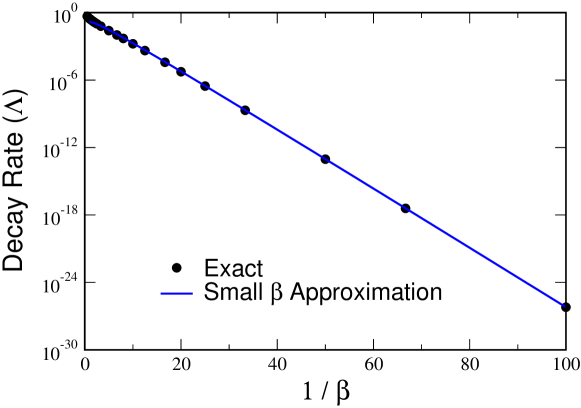
Figure 2: Decay rate vs. $1/\beta$, for the basic model, Eq. (1), with $\alpha=1$, together with the analytic approximation, Eq. (35). Here and in all other figures, the numerical calculation of the decay rate was performed using a quadruple-precision version of the sparse matrix eigenvalue solver ARPACK,arpack applied to the master equation transition matrix, with the absorbing state eliminated.

With this result for $Q_{n}$ in hand, we can finish the matching procedure. For $n\ll\alpha/\beta$, $\Lambda_{n}$ is large as we noted, and

$$Q_{n}\approx A\frac{\sqrt{2}\alpha}{\beta n}$$ (31)

Comparing to the recursion relation results, we have

$$A = P_{2}\frac{\beta^{2}}{2\alpha^{2}}$$ (32)

$$= P_{1}\sqrt{\frac{\beta^{3}}{4\pi\alpha^{3}}}$$

This fixes the ratio of $P_{1}$ to $P_{2}$, which is precisely that which makes $\ln(P_{n})$ a smooth function. About the maximum, $\Lambda_{n}\approx 1$, so that $Q_{n}\approx 4A/\sqrt{3}$, and

$$P_{n}\approx\frac{2}{\sqrt{3}}\left(\frac{\beta}{\alpha}\right)^{2}P_{2}e^{\Delta S}e^{-y^{2}/3}$$ (33)

The sum over $P_{n}$ is dominated by this FP Gaussian, and so, replacing the sum by and integral, we get

$$P_{\it tot}\approx 2\sqrt{\pi}\left(\frac{\beta}{\alpha}\right)^{3/2}P_{2}e^{\Delta S}$$ (34)

The decay rate $\Gamma$ is then

$$\Gamma=\beta\frac{P_{2}}{P_{\it tot}}\approx\sqrt{\frac{\alpha^{3}}{4\pi\beta}}e^{-2\alpha(1-\ln(2))/\beta}$$ (35)

This result is plotted in Fig. 2, where we see the agreement is excellent for small $\beta$. As $\Gamma$ varies by so many orders of magnitude over the scale of the graph, it is impossible to see from this the role of the prefactor. In Fig. 3, we plot the ratio of $\Gamma$ to $e^{\Delta S}$ as a function of $\beta$. We see the accuracy is quite good and gets better as $\beta$ gets smaller, as expected. This prefactor is, it should be noted, quite different from the factor $\alpha$ conjectured in Ref. ek . In Fig. 1, we present the graph of $P_{n}$ together with the WKB, Fokker-Planck, and low/intermediate $n$ approximations. We see that the WKB approximation is excellent everywhere, whereas the other approximations are more limited in their range of validity. In particular, the Fokker-Planck results is a serious overestimate of of the low $n$ probability, and an equally bad underestimate of the large $n$ probability. As the WKB and exact results cannot be distinguished on the scale of the figure, in Fig. 4 we present the ratio of the WKB to the exact result for $\alpha=1$, $\beta=0.01$. We see that the WKB approximation is good to the expected few percent level, with it degrading slightly for very small $n$. Given that the WKB approximation is a large-$n$ approximation, that it does as well as it does at low-$n$ is a undeserved present, and a consequence of the remarkable accuracy of Stirling’s formula down to $n=1$.

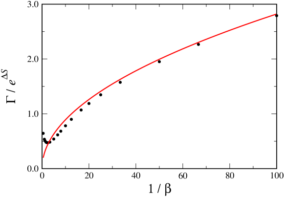
Figure 3: Ratio of $\Gamma$ to $e^{\Delta S}$, for the basic model, Eq. (1), compared to the WKB prediction, as a function of $\beta$, for $\alpha=1$.

Figure 4: Ratio of the WKB approximation for $P_{n}$ to the exact result for the basic model, Eq. (1) for $\beta=0.01$, $\alpha=1$.

For completeness, we note that it is possible to derive a large $\beta$ expansion of $\Gamma$ as well. This is easily done by truncating the master equation matrix and computing its determinant as a power series in $\alpha/\beta$, then solving for $\Gamma$ order by order. One finds

$$\Gamma\approx\alpha-2\frac{\alpha^{2}}{\beta}+\frac{10}{3}\frac{\alpha^{3}}{\beta^{2}}-\frac{38}{9}\frac{\alpha^{4}}{\beta^{3}}+\frac{242}{135}\frac{\alpha^{5}}{\beta^{4}}$$ (36)

It seems clear that this series has at best a finite radius of convergence. Both large and small $\beta$ limits are compared to the exact results in Fig. 5.

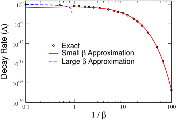
Figure 5: Decay rate vs. $1/\beta$ for the basic model, Eq. (1), with $\alpha=1$, together with the large $\beta$ approximation, Eq. (36), and the small $\beta$ approximation, Eq. (35).

II Parity-Preserving Model

In this section we will discuss the case where birth is to ”twins”, so that the even-odd parity of the number of particles is preserved. Here, a series of mathematical ”miracles” occur, which allow for a simple calculation of the extinction rate (for the case of an initial even number of particles) without recourse to the WKB method. Furthermore, we present a solution of the probability distribution to all orders in $\beta/\alpha$, so that the corrections are exponentially small. We also calculate the extinction rate to all orders in perturbation theory and manage to resum this divergent asymptotic series to obtain results correct to within exponentially small terms.

The model,

$$P \stackrel{{\scriptstyle\alpha/2}}{{\to}} 3P$$

$$P+P \stackrel{{\scriptstyle\beta}}{{\to}} 0$$ (37)

conserves the even/odd parity of the number of particles, so if the system is initialized with an odd number of particles it can never go extinct, instead reaching a steady-state. If the system is initialized with an even number of particles, on the other hand, the system can go extinct, with the survival probability decaying again as $e^{-\Gamma t}$, with $\Gamma$ exponentially small for small $\beta$. It should be noted that the mean-field equation for the model is the exact same as that of the original model above.

We again start with the master equation, which now reads:

$$\dot{P}_{n}=-\Gamma P_{n}=\frac{\alpha}{2}\left[-nP_{n}+(n-2)P_{n-2}\right]+\frac{\beta}{2}\left[-n(n-1)P_{n}+(n+2)(n+1)P_{n+2}\right]$$ (38)

As above, $\Gamma$ is exponentially small, and we may drop this term altogether. We again tackle the master equation by exploiting the fast growth of the $P_{n}$’s for not too large $n$. This observation allows us to drop the second $\alpha$ term and the first $\beta$ term, yielding the recursion relation

$$P_{n+2}=\left(\frac{\alpha}{\beta}\right)\frac{n}{(n+1)(n+2)}P_{n}$$ (39)

which, up to a factor of 2, is the same as the approximate recursion relation we previously encountered. Now, however, the parity conservation implies that only the even terms are nonzero, with the odd terms being exactly decoupled. The recursion relation has the solution

$$P_{2k}=\left(\frac{\alpha}{\beta}\right)^{k-1}\frac{(k-1)!2^{k}}{(2k)!}P_{2}$$ (40)

In principle, we should have to match this solution to the WKB solution, as we did in the nonparity case. The first miracle we encounter is that in fact the solution Eq. (40) is accurate throughout the Fokker-Planck region. To see this, note that for $n=\alpha/\beta+y\sqrt{\alpha/\beta}$, $y\sim O(1)$, the asymptotic expansion of $P_{n}$ is

$$P_{n}\approx\sqrt{2}\left(\frac{\beta}{\alpha}\right)^{2}e^{\alpha/2\beta}P_{2}e^{-y^{2}/4}$$ (41)

It is straightforward to verify that this is the solution of the Fokker-Planck equation:

$$0=\alpha\left(\frac{d}{dy}(yP)+2\frac{d^{2}}{dy^{2}}P\right)$$ (42)

It should be noted for the record that while Eq. (40) is an accurate representation of $P_{n}$ from $n=2$ till past the peak, the Fokker-Planck Gaussian is again only valid in the peak region.

Thus, we can use Eq. (40) to calculate $P_{\it tot}\equiv\sum_{k}P_{2k}$. We find

$$P_{\it tot}\approx P_{2}\sum_{k=1}^{\infty}\left(\frac{\alpha}{\beta}\right)^{k-1}\frac{(k-1)!2^{k}}{(2k)!}={}_{2}F_{2}(1,1;\frac{3}{2},2;\frac{\alpha}{2\beta})P_{2}$$ (43)

For the moment, what is important is the leading order asymptotics of this, which can be calculated directly by applying Laplace’s method to the sum. This is equivalent to integrating the Gaussian, and gives

$$P_{\it tot}\approx\sqrt{2\pi}\left(\frac{\beta}{\alpha}\right)^{3/2}e^{\alpha/2\beta}P_{2}$$ (44)

We are essentially done. The rate of probability flux out to the absorbing state is $\beta P_{2}$, which equals $\Gamma P_{\it tot}$. Thus,

$$\Gamma=\frac{\beta P_{2}}{P_{\it tot}}\approx\frac{\beta}{\sqrt{2\pi}\left(\frac{\beta}{\alpha}\right)^{3/2}e^{\alpha/2\beta}}=\sqrt{\frac{\alpha^{3}}{2\pi\beta}}e^{-\alpha/2\beta}$$ (45)

Note again that this is much smaller than the naive Fokker-Planck answer, which is proportional to $e^{-\alpha/4\beta}$.

We can actually proceed to compute the corrections to this formula. One source of corrections is using the asymptotics of ${}_{2}F_{2}$. The full asymptotics of ${}_{2}F_{2}$ for large argument are very beautiful:

$${}_{2}F_{2}(1,1;\frac{3}{2},2;x)\approx\sqrt{\frac{\pi}{4x^{3}}}e^{x}\left(1+\sum_{k=1}^{\infty}\frac{(2k-1)!!}{(2x)^{k}}\right)$$ (46)

This is obviously a divergent series, and alternatively represents a resummation of the series. This result is easily proven by substituting it in the Hypergeometric Differential Equation.

The second source of the corrections is the corrections to the $P_{n}$’s due to the terms we dropped in the master equation. The structure here is also strikingly beautiful. If we denote our zeroth-order approximation of $P_{n}$ by $P_{n}^{0}$, we find

$$P_{4} = P_{4}^{0}\left(1+\frac{\beta}{\alpha}\right)$$

$$P_{6} = P_{6}^{0}\left(1+\frac{\beta}{\alpha}+3\left(\frac{\beta}{\alpha}\right)^{2}\right)$$

$$P_{8} = P_{8}^{0}\left(1+\frac{\beta}{\alpha}+3\left(\frac{\beta}{\alpha}\right)^{2}+15\left(\frac{\beta}{\alpha}\right)^{3}\right)$$ (47)

The general trend is obvious:

$$P_{2k}=P_{2k}^{0}\left(1+\sum_{m=1}^{k-1}(2m-1)!!\left(\frac{\beta}{\alpha}\right)^{m}\right)$$ (48)

Plugging this into the master equation shows that this is an exact solution (for $\Gamma=0$, of course). Now, up to exponentially small corrections, $P_{\it tot}$ is just multiplied by the correction factor:

$$P_{\it tot} = P_{\it tot}^{0}\left(1+\sum_{m=1}^{\infty}(2m-1)!!\left(\frac{\beta}{\alpha}\right)^{m}\right)$$ (49)

$$= P_{\it tot}^{0}\sqrt{\frac{\alpha^{3}}{2\pi\beta^{3}}}e^{-\alpha/2\beta}{}_{2}F_{2}(1,1;\frac{3}{2},2;\frac{\alpha}{2\beta})$$

The final result for $\Gamma$ is

$$\Gamma\approx\frac{\sqrt{2\pi\beta^{5}/\alpha^{3}}}{\left[{}_{2}F_{2}(1,1;\frac{3}{2},2;\frac{\alpha}{2\beta})\right]^{2}}e^{\alpha/2\beta}$$ (50)

Even though this answer is a resummation of the full asymptotic series, it is nevertheless not exact. The correction terms however are exponentially small, (relative to the exponentially small extinction rate) going like $e^{-\alpha/\beta}$. This can be seen in the following graph, where we plot the relative error, comparing to an essentially exact numerical calculation (using extended precision arithmetic in Maple). Thus, for example, the error for $\alpha/\beta=100$ is six parts in $10^{21}$!

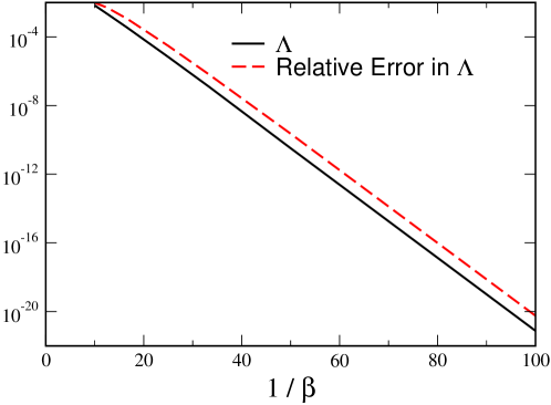
Figure 6: Extinction rate $\Gamma$ and the relative error between the approximation, Eq. (50), and the exact value as a function of $1/\beta$ for $\alpha=1$.

For completeness, we also briefly write down the WKB solution. Firstly,

$$n(\Lambda)=\frac{\alpha}{\beta\Lambda^{2}}$$ (51)

so that

$$\Delta S=\int_{1}^{\infty}\frac{n}{\Lambda}d\Lambda=\frac{\alpha}{2\beta}$$ (52)

Also,

$$S_{n}=\frac{n}{2}\left[\ln(\alpha/\beta)+1-\ln(n)\right]$$ (53)

The solution for $Q_{n}$ is the simple result

$$Q_{n}=A\Lambda^{2}$$ (54)

All this can be seen to agree with our recursion relation solution. In fact, it implies that the recursion relation solution is valid everywhere, even past the FP regime.

One can again calculate the large $\beta$ limit of the decay rate. The first few terms of this series are:

$$\Gamma=\beta-\frac{\alpha}{5}+\frac{12\alpha^{2}}{875\beta}-\frac{4\alpha^{3}}{21875\beta^{2}}-\frac{972\alpha^{4}}{58953125\beta^{3}}+\frac{24964\alpha^{5}}{95798828125\beta^{4}}$$ (55)

It would appear likely that this series is actually convergent. In any case, together with the small $\beta/\alpha$ results above, they cover the entire range of parameters, as can be seen in Fig. 7.

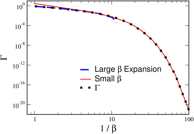
Figure 7: Decay rate $\Gamma$ for the parity conserving model, compared to the small $\beta$ result, Eq. (50), and the large $\beta$ power-series expansion, Eq. (55). The agreement between these analytical expressions and the exact results is so good in their respective spheres of validity, that the deviations are only visible quite far outside these areas.

III General Nonparity Model

Let us extend, now, our original, non-parity preserving, model to include a third process, the spontaneous death of particles at a rate $\gamma<\alpha$. Such a process appears naturally in many systems, from populations of animals (where $\gamma$ is the death rate of an individual) to the spread of a disease (where it correspond to a recovery of an infected agent, like in the SIR model 3 ). We present the physical optics solution for this case also, again confirming it by comparison to the direct numerical solution.

Adding the spontaneous decay of particles:

$$P\stackrel{{\scriptstyle\gamma}}{{\to}}0$$ (56)

to our basic model, Eq. (1), changes both the mean field and the fluctuations. At the mean-field level this is equivalent to a simple change of the effective growth rate, $\alpha$ of $\alpha_{\it eff}=\alpha-\gamma$, but this scaling is not true anymore if the fluctuations are taken into account. The master equation now reads:

$$\dot{P}_{n}=\alpha\left[-nP_{n}+(n-1)P_{n-1}\right]+\frac{\beta}{2}\left[-n(n-1)P_{n}+(n+2)(n+1)P_{n+2}\right]+\gamma\left[-nP_{n}+(n+1)P_{n+1}\right].$$ (57)

We start this time with the WKB solution. As before, the WKB ansatz yields an equation for $\Lambda_{n}$, namely

$$0 = \left(\frac{1}{2\Lambda_{n}}\right)\left[2\alpha\left(-\Lambda_{n}+1\right)+\beta n\left(-\Lambda_{n}+\Lambda_{n}^{3}\right)+2\gamma\left(-\Lambda_{n}+\Lambda_{n}^{2}\right)\right]$$ (58)

$$= \left(\frac{\Lambda_{n}-1}{2\Lambda_{n}}\right)\left[-2\alpha+\beta n\Lambda_{n}(\Lambda_{n}+1)+2\gamma\Lambda_{n}\right]$$

with the solution

$$\Lambda_{n}=\frac{\sqrt{(\beta n+2\gamma)^{2}+8\alpha\beta n}-2\gamma-\beta n}{2\beta n}$$ (59)

Now, $\Lambda$ approaches the finite limit, $\alpha/\gamma$ as $n$ goes to 0, in contrast to the previous cases. Thus, we cannot solve the low-$n$ recursion relation by assuming that the $P_{n}$ are increasing very rapidly. Rather, now $\beta$ is irrelevant for low $n$, and we have to solve the $\beta=0$ recursion. This is readily solved, for example by generating function techniques, and yields

$$P_{n}=\frac{\gamma}{n(\alpha-\gamma)}\left[\left(\frac{\alpha}{\gamma}\right)^{n}-1\right]P_{1}$$ (60)

Indeed, for large $n$ $P_{n}$ grows geometrically, with the ratio $\alpha/\gamma$, agreeing with the small $n$ WKB.

We can now proceed with the remainder of the WKB procedure. As before, it is more convenient to work with $n(\Lambda)$, given by

$$n(\Lambda)=\left(\frac{2}{\beta}\right)\frac{\alpha-\gamma\Lambda}{\Lambda(\Lambda+1)}$$ (61)

We see that in the mean-field regime, $\Lambda\approx 1$, the entire $\gamma$ dependence is through $\alpha_{\it eff}$. Away from this limit, however, the situation is more complicated.

Now, as before, $S_{n}$ is given by

$$S_{n} = S_{0}-\left[n(\Lambda)\ln(\Lambda)\rule{0.0pt}{12.0pt}\right]_{\Lambda}^{\alpha/\gamma}+\int_{\Lambda}^{\alpha/\gamma}\frac{n(\Lambda}{\Lambda}d\Lambda$$ (62)

$$= S_{0}+n\ln(\Lambda)+\frac{2(\alpha-\gamma\Lambda)}{\beta\Lambda}-\frac{2(\alpha+\gamma)}{\beta}\left(\ln\left(\frac{\Lambda+1}{\Lambda}\right)-\ln\left(\frac{\alpha+\gamma}{\alpha}\right)\right)$$

In particular,

$$\Delta S=\frac{2(\alpha-\gamma)}{\beta}+\frac{2(\alpha+\gamma)}{\beta}\ln\left(\frac{\alpha+\gamma}{2\alpha}\right)$$ (63)

We exhibit $\Delta S$ as a function of $\gamma$ for fixed $\alpha$ in Fig. 8. We see that $\Delta S$ decreases with increasing $\gamma$, vanishing quadratically as $\gamma$ approaches the threshold value of $\alpha$. Also interesting is the dependence of $\Delta S$ as a function of $\gamma$, for fixed $\alpha_{\it eff}$. This is show in Fig. 9. We see that as $\gamma$ increases, at fixed $\alpha_{\it eff}$, $\Delta S$ decreases, leading to a faster decay rate due to increased fluctuations. For large $\gamma$, in fact, $\Delta S$ vanishes as $\alpha_{\it eff}/(2\beta\gamma)$.

Figure 8: $2\beta\Delta S/\alpha$ as a function of $\gamma$, for fixed $\alpha$.

Figure 9: $2\beta\Delta S/\alpha_{\it eff}$ as a function of $\gamma$, for fixed $\alpha_{\it eff}$.

We now are in a position to continue to the calculation of $Q_{n}=e^{S_{1}(n)}$. The equation is

$$0 = \alpha\left[-n+\frac{n}{\Lambda_{n}}\left(1-S_{1}^{\prime}+\frac{1}{2}S_{0}^{\prime\prime}-\frac{1}{n}\right)\right]$$ (64)

$${}+\frac{\beta}{2}\left[-n^{2}+n+n^{2}\Lambda_{n}^{2}\left(1+2S_{1}^{\prime}+2S_{0}^{\prime\prime}+\frac{3}{n}\right)\right]$$

$${}+\gamma\left[-n+n\Lambda_{n}\left(1+S_{1}^{\prime}+\frac{1}{2}S_{0}^{\prime\prime}+\frac{1}{n}\right)\right]$$

which simplifies to, using $S^{\prime\prime}=1/(\Lambda n^{\prime}(\Lambda))$,

$$\left[\frac{\alpha}{\Lambda}-\beta n\Lambda^{2}-\gamma\Lambda\right]\frac{d}{d\Lambda}S_{1}=\frac{1}{2\Lambda}\left[\frac{\alpha}{\Lambda}+2\beta n\Lambda^{2}+\gamma\Lambda\right]+\frac{n^{\prime}(\Lambda)}{2n}\left[-\frac{2\alpha}{\Lambda}+\beta n+3\beta n\Lambda^{2}+2\gamma\Lambda\right]$$ (65)

This has the solution

$$Q_{n}=A\frac{\sqrt{\alpha^{3}\Lambda_{n}}(\Lambda_{n}+1)^{2}}{(\alpha-\gamma\Lambda_{n})\sqrt{\alpha(2\Lambda_{n}+1)-\gamma\Lambda_{n}^{2}}}$$ (66)

where we have inserted the factor $\sqrt{\alpha^{3}}$ so the definition of $A$ reduces to that used in the $\gamma=0$ case.

The last step is to match to the low-$n$ recursion relation solution. For $\beta n\ll 1$, the WKB solution reduces to

$$P_{n}\approx\frac{2A\sqrt{\alpha(\alpha+\gamma)}}{\beta n}\left(\frac{\alpha}{\gamma}\right)^{n}$$ (67)

Comparing this to Eq. (60), we get

$$A=\frac{\gamma\beta}{2(\alpha-\gamma)\sqrt{\alpha(\alpha+\gamma)}}P_{1}$$ (68)

We now need to calculate $P_{\it tot}$. Near the stable point, $n=(\alpha-\gamma)/\beta$,

$$P_{n}=4\sqrt{\frac{\alpha^{3}}{3\alpha-\gamma}}\frac{A}{\alpha-\gamma}e^{\Delta S}e^{-\frac{\beta}{3\alpha-\gamma}\left(n-\frac{\alpha-\gamma}{\beta}\right)^{2}}$$ (69)

which gives

$$P_{\it tot} = 4\sqrt{\frac{\pi\alpha^{3}}{\beta}}\frac{A}{\alpha-\gamma}e^{\Delta S}$$ (70)

$$= \sqrt{\frac{\pi\beta}{\alpha+\gamma}}\frac{2\alpha\gamma}{(\alpha-\gamma)^{2}}P_{1}e^{\Delta S}$$

The total probability flux out of the system is $\gamma P_{1}+\beta P_{2}$. Since $P_{2}$ is of order 1 relative to $P_{1}$, the $\beta$ contribution to the flux is negligible, and so

$$\Gamma=\frac{\gamma P_{1}}{P_{\it tot}}=\sqrt{\frac{\alpha+\gamma}{\pi\beta}}\frac{(\alpha-\gamma)^{2}}{2\alpha}e^{-\Delta S}$$ (71)

This result is tested against the exact numerical answer in Fig. 10. The results are again quite good, with the quality decreasing as $\gamma$ approaches $\alpha$ (for fixed $\beta$) as expected due to the decreasing equilibrium number of particles. The astute reader will note that our expression for $\Gamma$ reduces in the $\gamma\to 0$ limit to our $\gamma=0$ result above, even though some intermediate expressions (for example, the probability flux) do not correspond. We also note that the maximum value of $\Lambda$ is $\alpha/\gamma$, which approaches 1 as $\gamma$ approaches the threshold value of $\alpha$. Thus, near threshold, the Fokker-Planck equation and the WKB treatment coincide. Of course, this solution still has to be matched to the low/intermediate-$n$ solution to obtain the correct prefactor.

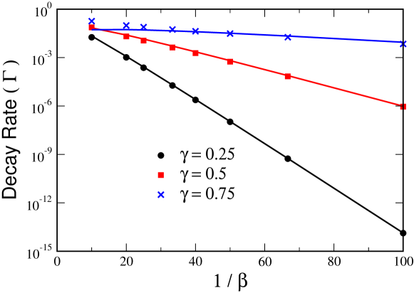
Figure 10: The calculated decay rate $\Gamma$ as a function of $1/\beta$, Eq. (71) for $\alpha=1$, $\gamma=0.25$, $0.5$, and $0.75$ (solid line) together with the exact numerical results (markers).

It should also be noted that Doering, et al.,b investigated a class of models wherein all transitions are single-particle transitions, as opposed to the models investigated herein, which include a 2 particle annihilation process. This entire class of models can also be easily treated via our WKB method, and yields identical results to those of Doering, et al. Writing the birth term in the master equation by $\alpha_{n}$ and the death term by $\gamma_{n}$, the WKB solution can be written down for a very broad class of models where $\alpha_{n}=(1/\beta)\tilde{\alpha}(\beta n)$ and $\gamma_{n}=(1/\beta)\tilde{\beta}(n)$, and $\tilde{\alpha}$, $\tilde{\beta}$ are smooth functions. In this case, the system admits a macroscopic metastable state with a large number of particles for small $\beta$. In particular, we find

$$\Lambda_{n}=\frac{\alpha_{n}}{\gamma_{n}}$$ (72)

so that

$$S_{n}=\int_{0}^{n}\ln(\Lambda_{n})dn$$ (73)

The $Q_{n}$ factor is:

$$Q_{n}=\frac{A}{\sqrt{\alpha_{n}\gamma_{n}}}$$ (74)

which, upon matching to the low/intermediate-$n$ result gives (up to an obvious typographical error) the result in Doering, et al. The advantage of the WKB method is that it generalizes to the multi-particle transition case.

IV Threshold case and the lifetime of a neutral mutation

In that section let us consider the threshold case, $\alpha=\gamma$. This case corresponds to the dynamics of a neutral mutation and has recently become the focus of extensive research, mainly in connection with Hubbell’s unified neutral theory of biodiversity and biogeography.4 Here, as we already saw for the near-threshold case, the $P_{n}$’s are smooth and allow for a Fokker-Planck treatment. However, in this case the decay rate $\Gamma$ is not exponentially small, and so cannot be ignored. First, let us consider what happens in the absence of $\beta$. This problem was worked out by Pechenik and Levine.PL They find that the mean number of particles is conserved and the variance grows linearly in time. Furthermore, the system exhibits a power-law ($1/t$) convergence to the empty state, and not an exponential dependence. This is indicative of a scale invariance in the problem. The $\beta$ term serves to break this scale invariance, and gives a well-defined scale for the number of particles (for those replicas which still survive). The original Fokker-Planck equation (ignoring boundary terms) was

$$\frac{\partial P}{\partial t}=\alpha\frac{\partial^{2}}{\partial n^{2}}(nP)$$ (75)

The $\beta$ process introduces two new terms into the FP equation, arising from the Taylor expansion of $\frac{1}{2}\beta\left(-n(n-1)P(n)+(n+2)(n+1)P(n+2)\right)$ in the master equation. The first of these terms is a drift term, $\beta\frac{\partial}{\partial n}(n^{2}P)$. This is responsible for the term in the mean-field equation. The second term is a diffusion term. If we assume $\beta$ small, then the additional diffusion induced by $\beta$ can be ignored, and we are left with only the drift term. The new FP equation now reads

$$\frac{\partial P}{\partial t}=-\Lambda P=\alpha\frac{\partial^{2}}{\partial n^{2}}(nP)+\beta\frac{\partial}{\partial n}(n^{2}P)$$ (76)

We have assumed the time dependence is exponential, and are looking for the smallest eigenvalue $\Lambda$. We shall see that $\Lambda$ vanishes in the $\beta\to 0$ limit, consistent with the power-law behavior found by P-L.

It is useful to transform the FP equation to Shroedinger form. The first step in this process is to change variables to $x\equiv\sqrt{n}$. This yields the equation

$$-\alpha P^{\prime\prime}-(\frac{3\alpha}{x}+2\beta x^{3})P^{\prime}-8\beta x^{2}P=4\Gamma P$$ (77)

The next step is a similarity transformation to eliminate the first derivative

$$P\equiv x^{-3/2}e^{-\beta x^{4}/4\alpha}Q$$ (78)

yielding the Schroedinger equation

$$-Q^{\prime\prime}+\left(\frac{3}{4x^{2}}-\frac{2\beta x^{2}}{\alpha}+\frac{\beta^{2}x^{6}}{\alpha^{2}}\right)Q=\frac{4\Gamma}{\alpha}Q$$ (79)

Clearly, in the absence of $\beta$ there is no bound state. Rather there is a continuum that starts at zero. The potential with $\beta$ has a single minimum, which is negative. Nevertheless, the ground state energy is positive, yielding a decay rate. The scaling of the decay rate is clear; by rescaling $y\equiv(\beta/\alpha)^{1/4}x$, $\beta$ and $\alpha$ disappear from the equation, with the decay rate scaling as $\sqrt{\alpha\beta}$. As advertised, we verify the vanishing of $\Lambda$ with $\beta$. The presence of $\beta$ has set the scale of (the surviving) $n$’s, namely $\sqrt{\alpha/\beta}$, which is large for small $\beta$. Lastly, the $1/x^{2}$ nature of the $\alpha$ potential is clearly a result of the scale-free nature of the $\beta=0$ problem. To get the prefactor multiplying the $\sqrt{\beta}$, we have to numerically solve the rescaled Shroedinger equation, (i.e., Eq. (79) with $\alpha=\beta=1$) yielding the result

$$\Gamma=1.111\sqrt{\alpha\beta}$$ (80)

The resulting scaled $P_{n}$ is shown in Fig. 11, together with the rescaled exact numerical solution of the master equation for $\beta=0.01$. We see that $P_{n}$ is strongly peaked at the origin, corresponding to the zero particle mean-field solution.

]

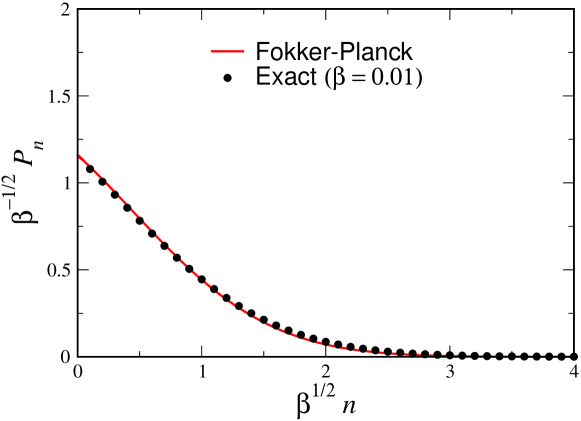
Figure 11: Rescaled probability distribution $\beta^{-1/2}P_{n}$ as a function of $\beta^{1/2}n$ for the case $\alpha=\gamma=1$, $\beta=0.01$, together with the numerical solution of the Fokker-Planck equation.

The scaling with $\beta$ we obtained is the same as found by Doering, et al. However, as opposed to the other cases examined herein, the prefactor is different as now the mean time to extinction is not simply the inverse of the decay rate. This is due to the fact that all the eigenvalues of the master equation scale as $\sqrt{\beta}$, whereas the other cases exhibited a single exponentially small eigenvalue.

V Conclusions

We have solved for the fluctuation-induced extinction rates of various models exhibiting a macroscopic metastable state. Our primary methodology is use the WKB method for difference equations to directly solve the master equation. This WKB solution then has to be matched to the low-$n$ $P_{n}$’s, since the WKB method is a large $n$ approximation. This technique is quite general and straightforward to implement, and produces quite accurate results as long as there are not too few particles in the metastable state. It reproduces the Doering, et al. results for the case of general one-particle transitions and generalizes to higher-order transitions. We have also shown the unique mathematical properties of the even/odd parity conserving model, where we are able to generate the full asymptotic expansion for the decay rate to all orders, and even to resum this divergent asymptotic series.

One interesting point which arises from this analysis is the sensitivity of the decay rate to the exact form of the microscopic dynamics. This is apparent in the very different dominant $e^{\Delta S}$ for the case of the parity and non-parity cases. This is also the case when one compares the logistic model with spontaneous decay studied in Section III, to the same model where the collision process $P+P\to 0$ is replaced by $P+P\to P$ at twice the rate. Even at the level of the Fokker-Planck dynamics valid near the metastable state, the widths of the distributions are different, with the variance $(3\alpha-\gamma)/2\beta$ being replaced by $\alpha/\beta$. The values of $\Delta S$ in the two cases are very different, where Eq. (63) for the two-particle annihilation should be compared to

$$\Delta S=\int_{0}^{(\alpha-\gamma)/\beta}\ln\left(\frac{\alpha}{\gamma+\beta n}\right)=\frac{\alpha-\gamma}{\beta}-\frac{\gamma}{\beta}\ln\left(\frac{\alpha}{\gamma}\right)$$ (81)

Thus, while the two expressions agree near threshold, where the Fokker-Planck description is sufficient, as $\gamma$ approaches 0, $\Delta S\to 2\alpha/\beta(1-\ln(2))$ for the two-particle annihilation case, as we saw in Section 1, whereas $\Delta S\to\alpha/\beta$, almost twice as large, for small $\gamma$ in the $P+P\to P$ case. Parenthetically, it should be noted that the small $\gamma$ limit is very singular in this latter case, as naively $\Gamma$ seems to diverge as $\gamma^{-1/2}$ for small $\gamma\ll\beta$. In general, for small $\beta$ and $\gamma$, the decay rate can be shown to be given by

$$\Gamma\approx\left(\frac{\alpha}{\beta}\right)^{\gamma/\beta}\frac{a}{\Gamma(\gamma/\beta)}e^{-\alpha/\beta}$$ (82)

as so indeed vanishes as $\gamma\to 0$, since there is no extinction in this case. In situations where the Fokker-Planck equation is valid all the way down to $n=0$, as we saw was the case at threshold, at least the problem is parameterized by only two parameters, the center and width of the Gaussian. However, in general, the entire function $n(\Lambda)$ is involved in the calculation of $\Delta S$. This should have important implications for the study of extinctions in the ecological community, for example, where reliable microscopic models are difficult if not impossible to obtain.

- (1) C.W. Gardiner, Handbook of Stochastic methods, Springer, Berlin 1985.
- (2) G.V. Grimm and C. Wissel, Oicos 105, 501 (2004)
- (3) P. Foley, Extinction models for local population, in Metapopulation Biology - Ecology, Genetics and Evolution, I.A. Hanski and M.E. Gilpin (Ed.) (Academic Press, London, 1997).
- (4) See, e.g., B. Drossel, Advances in Physics 50, 209 (2001) and references therein.
- (5) See, e.g., M. J. Keeling and B. T. Grenfell, Science 275, 65 (1997); M. Lipsitch et al., Science 300, 1966 (2003); J. O. Lloyd-Smith S. J. Schreiber, P. E. Kopp and W. M. Getz, Nature 438, 355 (2005); .
- (6) V. Elgart and A. Kamenev, Phys. Rev. E 70, 41106 (2004).
- (7) C.R. Doering, K.V. Sargsyan, and L.M. Sander, Multi- scale Model. and Simul. 3, 283 (2005).
- (8) M.I. Dykman, E. Mori, J. Ross, and P.M. Hunt, J. Chem. Phys. 100, 5735 (1994).
- (9) M. Assaf and B. Meerson, Phys. Rev. E 74, 041115 (2006).
- (10) S.P. Hubbell, The Unified Neutral Theory of Biodiversity and Biogeography. (Princeton University Press, Princeton, NJ, 2001).
- (11) M. Doi, J. Phys. A 9, 1465 (1976); L. Peliti, J. Physique 36, 1469 (1985).
- (12) J. L. Cardy and U. C. Tauber, Phys. Rev. Lett. 77, 4780 (1996); J. L. Cardy and U. C. Tauber, J. Stat. Phys. 90, 1 (1998).
- (13) C. M. Bender and S. A. Orszag, Advanced Mathematical Methods for Scientists and Engineers, (Springer, New York, 2005).
- (14) For details, see http://www.caam.rice.edu/software/ARPACK.
- (15) L. Pechenik and H. Levine, Phys. Rev. E 59, 3893 (1999).