Nucleotide Frequencies in Human Genome and Fibonacci Numbers

Abstract

This work presents a mathematical model that establishes an interesting connection between nucleotide frequencies in human single-stranded DNA and the famous Fibonacci’s numbers. The model relies on two assumptions. First, Chargaff’s second parity rule should be valid, and, second, the nucleotide frequencies should approach limit values when the number of bases is sufficiently large. Under these two hypotheses, it is possible to predict the human nucleotide frequencies with accuracy. It is noteworthy, that the predicted values are solutions of an optimization problem, which is commonplace in many nature’s phenomena.

$\Pi\rho\alpha\gamma\mu\alpha$ $\epsilon\iota\nu\alpha\iota$ $\alpha\rho\iota\theta\mu o\iota$

1 Introduction

The amount of available genome data is increasing very fast due the completion of a host of genome sequencing projects. The careful analysis of all these data is only beginning. The genome sequence by itself is meaningless, it is necessary to identify genes, proceed the annotation, and, if possible, get some understanding of the very process responsible by the sequence formation.

Less than $25\%$ of the fly genome is in coding regions, and the number falls to less than $3\%$ in humans [2]. It seems that the most part of eukaryotes genomes is “garbage” DNA. Nevertheless, recently, some evidences show that it is not the case. Mutations in noncoding regions were associated with cancer [7]. Consequently, the interest in noncoding regions has increased, and the role that those regions have in the whole genome demands a better comprehension.

The initial step in any genome analysis is to perform some simple statistical measures like frequencies and averages. These kind of research have been done even before the discovery of DNA structure, and allowed some striking scientific advances. For instance, in 1951, Chargaff [1] observed that, in any piece of double-stranded DNA, the frequencies of adenine and thymine are equal, and so are the frequencies of cytosine and guanine. In mathematical notation $P_{A}=P_{T}$ and $P_{C}=P_{G}$, where $P_{A},P_{C},P_{G}$ and $P_{T}$ denote the nucleotide frequencies of adenine, cytosine, guanine and thymine, respectively. This observation is known as Chargaff’s first parity rule. Watson and Crick, in 1953, were acquainted with Chargaff’s first parity rule, and used it to support their DNA double-helix model [8]. Furthermore, Chargaff also observed that the parity rule approximately holds in a single-stranded DNA, nonetheless the equality is not strict, but $P_{A}\cong P_{T}$ and $P_{C}\cong P_{G}$. This is known as Chargaff’s second parity rule. Possibly, the best explanation to this rule can be found in [4]. Chargaff’s second rule has been extensively tested [5] and proved to hold in the majority of the genome sequences.

A particular interesting case is found in human genome. We have tested the Chargaff’s second parity rule for each one of the 24 human chromosomes $(22+X+Y)$, and it is definitely valid. Moreover, notice that $P_{A}+P_{T}+P_{C}+P_{G}=1$ by definition (the sum of all frequencies must be equal to 1), and assuming Chargaff’s second parity rule, we get that $P_{A}+P_{C}\cong\frac{1}{2}$ or, equivalently, $P_{T}+P_{G}\cong\frac{1}{2}$, or any possible combination. If we plot the points $(P_{A},P_{C})$ for each human chromosome, we get another interesting fact: they are not evenly spread over the line $P_{A}+P_{C}=\frac{1}{2}$, but seem to be aggregated around some very precise values. In Figure 1, in red, the line $P_{A}+P_{C}=\frac{1}{2}$, and the green dots are the points $(P_{A},P_{C})$ for each human chromosome.

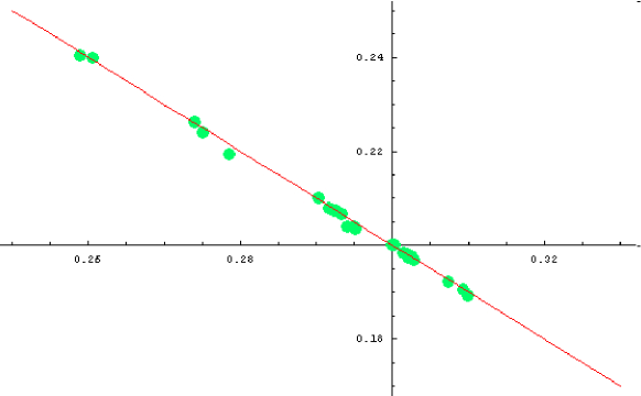
Figure 1: In red the line $P_{A}+P_{C}=\frac{1}{2}$, and in green the observed points $(P_{A},P_{C})$ for each human chromosome

Although this observation is not expected, it is not completely unusual. Many phenomena in nature show the same pattern, and some of them can be mathematically modeled. Usually, those mathematical models that describe nature’s phenomena involve optimization problems. It seems that nature is always trying to optimize itself in different contexts. Therefore, the following question emerges naturally: Is it possible to build a mathematical model that predicts or explain the observed frequencies?

Assuming that (i) the human nucleotide frequencies really tend to limit values when the number os bases is sufficiently large, and (ii) Chargaff’s second parity rule is valid, we derived a mathematical model that predicts the observed frequency values with accuracy.

2 Mathematical Model

In order to understand our model, it is necessary to introduce the Fibonacci numbers [3].

2.1 Fibonacci Numbers

In mathematics, one of the most famous integer sequence is without doubt the sequence $\{1,1,2,3,5,8,13,...\}$.

This sequence, called Fibonacci sequence, is obtained through the recurrence formula

$$F(n+2)=F(n+1)+F(n),$$ (1)

together with the initial conditions $F(1)=1$ and $F(2)=1$.

The Fibonacci sequence was first described, in the Occident, by Leonardo of Pisa, also known as Fibonacci, in his book Liber Abaci. The Fibonacci sequence appears in nature in different contexts: sea shell shapes, flower petals and seeds, etc.

It is related to the Golden Ratio, $\phi$, by the limit

$$\phi=\lim_{n\rightarrow\infty}\frac{F(n+1)}{F(n)}.$$ (2)

The Golden Ratio is associated to Beauty and Perfection, and for this reason it is conventional to find $\phi$ present in art (Leonardo da Vinci), architecture (Parthenon in Athens, for example) and music (notably in Bartók and Debussy). There is a plenty of written works about the Golden Ratio and the Fibonacci numbers.

2.2 Assumptions and Model

The main assumption of our model is that Chargaff’s second parity rule is valid in all human chromosomes. There are many different forms to state it mathematically. We’ve decided to do it in the following way: the division of the frequency of one nucleotide by the sum of the frequencies of the remaining nucleotides is in the proportion of three Fibonacci numbers. Of course, the choice of Fibonacci numbers were based in their generalized occurence in nature; although, we’ve also tried other sets of numbers, but with no success.

Consider the three Fibonacci numbers below

$$\left\{F(n),F(n+1),F(n+k)\right\}.$$ (3)

where $n$ is a sufficiently large number and $k=0,1,2,3,..,N$ ( $N$ is finite number).

Therefore, we can write the main assumption as

$$\frac{x(n)}{y(n)+z(n)+w(n)}\propto\frac{F(n)}{F(n+k)},$$ (4)

$$\frac{y(n)}{x(n)+z(n)+w(n)}\propto\frac{F(n+1)}{F(n+k)},$$ (5)

$$\frac{z(n)}{x(n)+y(n)+w(n)}\propto\frac{F(n)}{F(n+k)},$$ (6)

$$\frac{w(n)}{x(n)+y(n)+z(n)}\propto\frac{F(n+1)}{F(n+k)},$$ (7)

where $x(n),y(n),z(n)$ and $w(n)$ represent the nucleotide frequencies, without any a priori association, when the number of nucleotide bases is $n$, i. e., $x(n)=\frac{x_{n}}{n}$, where $x_{n}$ stands for the number of nucleotide $x$.

It is not straightforward to recognize Chargaff’s second parity rule in equations (4) - (7). One way to grasp the idea behind the formulas is to note that equations (4) and (6) are proportional to the same quotient $\left(\frac{F(n)}{F(n+k)}\right)$, and the same can be said about equations (5) and (7). In next section, we will show how to get Chargaff’s second parity rule from the above equations.

2.2.1 Limit Values

Now, lets impose our second assumption, i. e., that the nucleotide frequencies tend to limit values when $n$ is sufficiently large. Mathematically, it can be written as

$$x=\lim_{n\rightarrow\infty}\frac{x_{n}}{n}$$ (8)

$$y=\lim_{n\rightarrow\infty}\frac{y_{n}}{n}$$ (9)

$$z=\lim_{n\rightarrow\infty}\frac{z_{n}}{n}$$ (10)

$$w=\lim_{n\rightarrow\infty}\frac{w_{n}}{n}$$ (11)

It is also necessary to understand what happens with the quotients $\frac{F(n)}{F(n+k)}$ and $\frac{F(n+1)}{F(n+k)}$ when $n\rightarrow\infty$.

Using equation (1) recursively, it is easy to get the following recurrence formula

$$F(n+k)=F(k)F(n+1)+F(k-1)F(n).$$ (12)

We are particularly interested in the cases where $n$, the numbers of bases, is large, and the quotient of the Fibonacci numbers tends to a limit.

Mathematically, this can be obtained as follows. Dividing (12) by $F(n+k)$, we get

$$1=F(k)\frac{F(n+1)}{F(n+k)}+F(k-1)\frac{F(n)}{F(n+k)}.$$ (13)

Taking the limit as $n\rightarrow\infty$,

$$1=F(k)\lim_{n\rightarrow\infty}\frac{F(n+1)}{F(n+k)}+F(k-1)\lim_{n\rightarrow\infty}\frac{F(n)}{F(n+k)},$$ (14)

We define

$$\lambda_{1,k}=\lim_{n\rightarrow\infty}\frac{F(n+1)}{F(n+k)}$$ (15)

and

$$\lambda_{2,k}=\lim_{n\rightarrow\infty}\frac{F(n)}{F(n+k)}$$ (16)

Notice that $\lambda_{1,k}$ and $\lambda_{2,k}$ are linked to the Golden Ratio by

$$\lambda_{1,k}=\phi^{1-k}$$ (17)

and

$$\lambda_{2,k}=\phi^{-k},$$ (18)

respectively.

Thus, the equation (14) can be written as

$$1=F(k)\lambda_{1,k}+F(k-1)\lambda_{2,k}$$ (19)

Finally, our model can be rewritten as

$$\frac{x}{y+z+w}=\lambda_{1,k},$$ (20)

$$\frac{y}{x+z+w}=\lambda_{2,k},$$ (21)

$$\frac{z}{x+y+w}=\lambda_{1,k},$$ (22)

$$\frac{w}{x+y+z}=\lambda_{2,k},$$ (23)

As noted before, $x$, $y$, $z$ and $w$ are frequencies, so we have

$$x+y+z+w=1.$$ (24)

Using equation (24), the equations (20)-(23), we get

$$\frac{x}{1-x}=\lambda_{1,k},$$ (25)

$$\frac{y}{1-y}=\lambda_{2,k},$$ (26)

$$\frac{z}{1-z}=\lambda_{1,k},$$ (27)

$$\frac{w}{1-w}=\lambda_{2,k},$$ (28)

Equations (25) and (27) imply that

$$x=z$$ (29)

and, analogously, equations (26) and (28) imply that

$$y=w$$ (30)

Equations (29) and (30) are the Chargaff’s second parity rule.

Moreover, an immediate consequence of equations (29), (30) and(24) is

$$x+y=\frac{1}{2}$$ (31)

2.3 Optimization Problem

Now, we have three equations in two variables

$$\frac{x}{1-x} = \lambda_{1,k}$$ (32)

$$\frac{y}{1-y} = \lambda_{2,k}$$ (33)

$$x+y = \frac{1}{2}$$ (34)

which can be rewritten as

$$x = \frac{\lambda_{1,k}}{1+\lambda_{1,k}}$$ (35)

$$y = \frac{\lambda_{2,k}}{1+\lambda_{2,k}}$$ (36)

$$x+y = \frac{1}{2}$$ (37)

This is a linear system, and, using equations (19) and (31), it is not difficult to show that it is inconsistent, independently, of $k$. In fact, only when $k\rightarrow\infty$, the system is consistent, but we are dealing with the cases where $k$ is finite.

The equation (31) must be satisfied because $x$ and $y$ are frequencies and, by definition, the equation (24) must hold. Therefore, we should try to minimize the difference between $x$ and $\frac{\lambda_{1,k}}{1+\lambda_{1,k}}$, and the difference between $y$ and $\frac{\lambda_{2,k}}{1+\lambda_{2,k}}$ under the condition that $x+y=\frac{1}{2}$.

This is a classical optimization problem, and can be mathematically stated as

$$\min_{x+y=\frac{1}{2}}f_{k}(x,y),$$ (38)

where

$$f_{k}(x,y)=\left(x-\frac{\lambda_{1,k}}{1+\lambda_{1,k}}\right)^{2}+\left(y-\frac{\lambda_{2,k}}{1+\lambda_{2,k}}\right)^{2}$$ (39)

This minimization problem is sufficiently easy to solve, because its objective function is quadratic and the Jacobian of the constraint is full rank, therefore the solution exists and is unique [6].

In Table 1 we list the solutions to the first $8$ values of $k$. It is not difficult to show that $(x,y)\rightarrow(0.25,0.25)$ as $k\rightarrow\infty$.

k	$x$	$x\cong$	$y$	$y\cong$
0	$\frac{3+\sqrt{5}}{8+4\sqrt{5}}$	0.3090	$\frac{1+\sqrt{5}}{8+4\sqrt{5}}$	0.1909
1	$\frac{3+\sqrt{5}}{8+4\sqrt{5}}$	0.3090	$\frac{1+\sqrt{5}}{8+4\sqrt{5}}$	0.1909
2	$\frac{127+57\sqrt{5}}{420+188\sqrt{5}}$	0.3027	$\frac{83+37\sqrt{5}}{420+188\sqrt{5}}$	0.1972
3	$\frac{161+72\sqrt{5}}{550+246\sqrt{5}}$	0.2927	$\frac{114+51\sqrt{5}}{550+246\sqrt{5}}$	0.2072
4	$\frac{881+392\sqrt{5}}{3126+1398\sqrt{5}}$	0.2818	$\frac{682+305\sqrt{5}}{3126+1398\sqrt{5}}$	0.2181
5	$\frac{20583+9205\sqrt{5}}{75588+33804\sqrt{5}}$	0.2723	$\frac{17211+7697\sqrt{5}}{75588+33804\sqrt{5}}$	0.2276
6	$\frac{15908+7070\sqrt{5}}{59665+26683\sqrt{5}}$	0.2649	$\frac{3(9349+4181\sqrt{5})}{119330+53366\sqrt{5}}$	0.2350
7	$\frac{100793+45076\sqrt{5}}{388045+173539\sqrt{5}}$	0.2597	$\frac{186459+83387\sqrt{5}}{776090+347078\sqrt{5}}$	0.2402

Table 1: Solutions of the optimization problem for different values of $k$

The values of Table 1 are in agreement with the observed frequencies in human chromosomes. In the next section, we will present the data that supports this mathematical model.

3 Results

We’ve performed a simple experiment using the nucleotide frequencies in human genome. The human genome data were obtained at NCBI. From time to time new human genome releases are deposited. We’ve used Build 35.1. It is important to note that only partial data is available for each chromosome, i.e., there are still missing sections (for example, chromosome 1 is supposed to have about 263 million bases, but only about 220 million bases were available). This information is relevant because it can explain some minor deviations from the predicted values.

3.1 Human Nucleotide Frequencies

This experiment consisted in calculating the nucleotide frequencies in all 24 human chromosomes. The results are summarized in the following table.

Chromosome	$P_{A}$	$P_{C}$	$P_{G}$	$P_{T}$	$k$
Chrom 1	0.2916	0.2080	0.2080	0.2922	3
Chrom 2	0.3000	0.2003	0.2005	0.2997	2
Chrom 3	0.3019	0.1980	0.1980	0.3020	2
Chrom 4	0.3093	0.1905	0.1906	0.3094	1
Chrom 5	0.3020	0.1974	0.1975	0.3011	2
Chrom 6	0.3024	0.1975	0.1976	0.3023	2
Chrom 7	0.2950	0.2040	0.2040	0.2951	3
Chrom 8	0.3002	0.2001	0.2000	0.2999	2
Chrom 9	0.2933	0.2067	0.2067	0.2931	3
Chrom 10	0.2922	0.2074	0.2074	0.2928	3
Chrom 11	0.2925	0.2072	0.2075	0.2926	3
Chrom 12	0.2950	0.2040	0.2033	0.2956	3
Chrom 13	0.3072	0.1922	0.1922	0.3080	1
Chrom 14	0.2951	0.2034	0.2039	0.2974	3
Chrom 15	0.2903	0.2101	0.2099	0.2895	3
Chrom 16	0.2750	0.2040	0.2040	0.2750	4
Chrom 17	0.2740	0.2261	0.2258	0.2713	5
Chrom 18	0.3014	0.1982	0.1985	0.3017	2
Chrom 19	0.2588	0.2403	0.2409	0.2598	7
Chrom 20	0.2785	0.2194	0.2202	0.2817	5
Chrom 21	0.2940	0.2040	0.2039	0.2952	3
Chrom 22	0.2605	0.2398	0.2397	0.2598	6
Chrom X	0.3027	0.1968	0.1967	0.3033	2
Chrom Y	0.3098	0.1893	0.1889	0.3118	1

Table 2: Nucleotide Frequencies for all human chromosomes

The nucleotide frequencies are clustered around the predicted values of Table 1. In Figure 2, we have in red the solutions of the optimization problem for different values of $k$, and in green the points $(P_{A},P_{C})$ for each one of the human chromosomes. The red circles have their centers in the solutions of the optimization problem and they have the same radius equal to $0.005$.

It is interesting to note that all the points $(P_{A},P_{C})$ are near ( less than $0.005$) to the predicted values.

The average values are $\mu_{P_{A}}=0.292$, $\mu_{P_{C}}=0.207$, $\mu_{P_{G}}=0.207$ and $\mu_{P_{T}}=0.292$, which are close to the optimization’s solution when $k=3$.

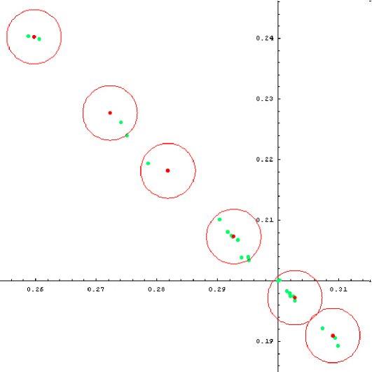
Figure 2: In red dots, the solutions of the optimization problem for different values of $k$. In green, the points $(P_{A},P_{C})$ for each one of the human chromosomes.

4 Conclusion

Using Chargaff’s second parity rule and assuming that the nucleotide frequencies tend to limit values when the number of nucleotide bases is sufficiently large, we’ve described a mathematical model that predicts the limit values of the human nucleotide frequencies with great accuracy. It is also interesting to note that the limit values are the results of an optimization problem, and it is commonly found in many phenomena in nature.

If our two hypotheses hold and our mathematical model is correct, then it is possible to make the following conjecture: the noncoding DNA regions play a major rule in the “optimization process” to reach the limit values predicted in our mathematical model. This conjecture is based on the fact that about $97\%$ of human genome is believed to be noncoding.

Acknowledgements

We are grateful to Dr. Bernard Maigret from Henry Poincaré University (Nancy - France), Dr. Robert Giegerich from Bielefeld University ( Bielefeld - Germany) and Dr. Nir Cohen from Campinas State University (Campinas - Brazil) for their valuable comments on our manuscript.

References

- [1] Chargaff, E. (1951);Struture and function of nucleic acids as cell constituents, Fed. Proc., 10, 654-659.
- [2] Do, J. H. and Choi D-K (2006); Computational Approaches to Gene Prediction, Journal of Microbiology, 44, 137-144.
- [3] Fibonacci, L. and Singler, L. E (Translator) (2002);Fibonacci’s Liber Abaci,New York, Ed. Springer-Verlag.
- [4] Forsdyke, D. R. and Bell, S. J. (2004);A discussion of the application of elementary principles to early chemical observations, Applied Bioinformatics,3,3-8.
- [5] Mitchell, D. and Bridge, R. (2006);A test of Chargaff’s second rule, BBRC, 340, 90-94.
- [6] Nocedal, J. and Wright, S. J. (2000);Numerical Optimization, Springer Series in Operations Research, New York, Ed. Springer-Verlag.
- [7] Schwartz, S., Alazzouzi, H. and Perucho M. (2006); Mutational dynamics in human tumors confirm the neutral intrinsic instability of the mitochondrial D-loop poly-cytidine repeat, Genes Chromosomes and Cancer, 8, 770-780.
- [8] Watson, J. D. and Crick, F. H. C. (1953); Molecular Structure of Nucleic Acids, Nature, 4356, 737.