Propagation of fluctuations in interaction networks governed by the law of mass action.

Abstract

Using an example of physical interactions between proteins, we study how perturbations propagate in interconnected networks whose equilibrium state is governed by the law of mass action. We introduce a comprehensive matrix formalism which predicts the response of this equilibrium to small changes in total concentrations of individual molecules, and explain it using a heuristic analogy to a current flow in a network of resistors. Our main conclusion is that on average changes in free concentrations exponentially decay with the distance from the source of perturbation. We then study how this decay is influenced by such factors as the topology of a network, binding strength, and correlations between concentrations of neighboring nodes. An exact analytic expression for the decay constant is obtained for the case of uniform interactions on the Bethe lattice. Our general findings are illustrated using a real biological network of protein-protein interactions in baker’s yeast with experimentally determined protein concentrations.

Equilibria in a broad class of microscopically reversible processes whose direct and reverse rates are proportional to the product of concentrations of participating substances is described by the Law of Mass Action (LMA). It has been rigorously proven that the unique steady state of such processes is completely defined by the set of initial concentrations and reaction constants [1]. Recently, it has become popular to visualize large sets of interacting substances as networks, where nodes and links correspond to the reactants and their propensity for pairwise interactions. One of the best-studied examples of such networks is that formed by all protein-protein physical interactions (pairwise bindings) in a given organism. The LMA determines the equilibrium free concentrations of individual proteins as well as those of hetero- and homo- dimers. A surprising feature observed in virtually all recent large-scale studies of these networks in a wide-ranging variety of biological organisms is their globally connected topology. Indeed, most pairs of protein nodes are linked to each other by relatively short chains of interactions. Total (bound plus unbound) concentrations of individual proteins are subject to both stochastic fluctuations due to the noise in their production and degradation as well as to systematic changes in response to external and internal stimuli. Such localized perturbation changes bound and free concentrations of immediate neighbors of the perturbed protein which in their turn influence their neighbors, etc. Thus a fluctuation in the total concentration of just one reactant to some degree affects free concentrations of all substances in the same connected component of the network. The propagation of fluctuations far away from their source presents a great threat of undesirable cross-talk between different functional processes, simultaneously taking place in an organism. Thus it is important to understand whether and how this propagation gets attenuated and under what conditions it is minimized. There also exist several anecdotal cases when changes in free concentrations propagating beyond the immediate neighbors of a perturbed protein are used for a meaningful biological regulation/signaling. Then a relevant question is under what conditions the propagation of the signal in a desirable direction is the least attenuated.

In this work we study how localized perturbations such as changes of concentrations of individual proteins affect the binding equilibrium at all nodes of a protein interaction network. Our main conclusion is that under a broad range of conditions such perturbations exponentially decay with the network distance away from the perturbed node. Luckily, this makes protein binding networks poor conduits for indiscriminately propagating fluctuations which would have led to undesirable cross-talk between biologically distinct pathways. On the other hand, under carefully selected conditions, a perturbation can propagate relatively far with a minimal attenuation. We first consider a general case of propagation of small perturbations in a network of an arbitrary topology, concentrations, and dissociation constants. Several simpler analytically tractable case studies follow.

Consider a network of pairwise interactions between $N$ distinct types of proteins (or any other molecules for that matter), where each protein corresponds to a vertex. The existence of a link between vertices $i$ and $j$ means that substances $i$ and $j$ interact to form a bound complex (hetero- or homo- dimer) $ij$. Throughout this paper we would consider only such dimers and ignore the existence of multi-protein complexes consisting of 3 or more proteins. However, we checked [2] that our main results could be easily extended to an arbitrary composition of complexes or even to a situation in which individual nodes combine with each other in reversible chemical reactions obeying the LMA.

The LMA dictates that free concentrations of proteins $F_{i}$ and those of dimers $D_{ij}$ obey

$${F}_{i}\;{F}_{j}=k_{ij}{D}_{ij},$$ (1)

where $k_{ij}$ is the corresponding dissociation constant. Adding the mass conservation one obtains the following system of equations that relates total concentrations $C_{i}$ of proteins to their free concentrations $F_{i}$,

$$C_{i}=F_{i}+\sum_{j\leftrightarrow i}D_{ij}=F_{i}+\sum_{j\leftrightarrow i}\frac{F_{i}F_{j}}{k_{ij}}\qquad.$$ (2)

Here and below the notation $\sum_{j\leftrightarrow i}$ means a sum over all vertices $j$ that are the network neighbors of the vertex $i$. In a general case of 4 or more interconnected interacting pairs this system of non-linear equations allows for only numerical solution. One particularly convenient computational method involves rewriting the Eq. (2) as

$$F_{i}=\frac{C_{i}}{1+\sum_{j\leftrightarrow i}F_{j}/k_{ij}}$$ (3)

and successively iterating it starting with $F_{i}=C_{i}$ until the LMA is satisfied with a desired precision. The proof presented in Ref. [1] guarantees the uniqueness of the solution found this way. Now consider a change in free concentrations $\delta F_{j}$ induced by a small perturbation of total concentrations $\delta C_{i}$. Linearization of Eq. (2) yields

$$\frac{\delta C_{i}}{C_{i}}=\sum_{j}\Lambda_{ij}\frac{\delta F_{j}}{F_{j}}\qquad,$$ (4)

with matrix $\hat{\Lambda}$ [3] given by

$$\Lambda_{ij}=A_{ij}\frac{D_{ij}}{C_{i}}+\delta_{ij}\qquad.$$ (5)

Here $A_{ij}$ is the adjacency matrix of the network. In case of multi-protein complexes consisting of more than 2 different proteins $D_{ij}$ should be replaced with the total concentration of all complexes containing both $i$ and $j$ among their constituents. It follows from Eqs. (4,5) that if the change in total concentration was limited to just one node $0$, the induced relative change of free concentration of any other node $i\neq 0$ satisfies

$$\frac{\delta F_{i}}{F_{i}}=-\sum_{j\leftrightarrow i}\frac{D_{ij}}{C_{i}}\frac{\delta F_{j}}{F_{j}}\qquad.$$ (6)

This equation shows that changes in free concentrations on nearest neighbors tend to be of the opposite sign. Also, since $\sum_{j\leftrightarrow i}D_{ij}/C_{i}=1-F_{i}/C_{i}<1$, the absolute magnitude of perturbation $|\delta F_{i}/F_{i}|$ on any node away from the source is less or equal than its maximal value among its neighbors: $\max_{j\leftrightarrow i}|\delta F_{j}/F_{j}|$. Bonds with higher $D_{ij}/C_{i}$ are better transmitters of perturbations from node $j$ to node $i$. Note, that this quantity is non-symmetric: The transmission along any particular edge is directional with preferred direction pointing from the higher total concentration to lower one.

Inverting (4) one obtains the desired expression for the linear response of any free concentration to an arbitrary perturbation in total concentrations:

$$\frac{\delta F_{i}}{F_{i}}=\sum_{j}\left({\hat{\Lambda}}^{-1}\right)_{ij}\frac{\delta C_{j}}{C_{j}}\qquad.$$ (7)

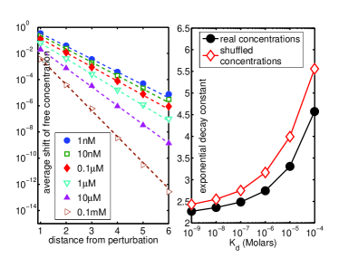
Figure 1: A) The average magnitude of normalized changes in free concentrations $|\delta F_{i}/F_{i}|$ per unit of $\delta C_{0}/C_{0}$ plotted as a function of the distance $l_{i0}$ from the perturbed node $0$. The propagation of perturbations (Eq. 7) was computed in a highly curated yeast PPI network [4] with real-life total concentrations of individual proteins [5] and dissociation constant $K_{d}$ increasing in 10-fold increments starting from $1$nM (or 34 molecules/cell) and up to 0.1mM (the steepest decaying curve).
B) The exponential decay constant $\gamma(K_{d})$ obtained from the best fit in the form $A\exp[-\gamma(K_{d})l_{i0}]$ to curves shown in the Panel A with the real-life concentrations (filled circles), and for randomly reshuffled concentrations (open diamonds).

As an application of the general theory outlined above we calculated the free concentrations $F_{i}$ and the linear response matrix ${\hat{\Lambda}}^{-1}$ in a realistic protein network of baker’s yeast Saccharomyces cerevisiae. A highly-curated set of protein-protein physical interactions from the BIOGRID dataset [4] was further restricted to include only interactions which were reported in at least two publications. Total concentrations of proteins for yeast grown in rich growth medium conditions were taken from a genome-wide experimental study [5]. The resulting dataset consists of 4185 interactions among 1740 proteins with total concentrations ranging between 50 and 1 million molecules/cell with median $\sim$ 3000 molecules/cell. In the absence of genome-wide information regarding the value of dissociation constants in our simulations we assume them all to be the same $k_{ij}=K_{d}$. We also tried simulations in which $k_{ij}$ are randomly drawn from a particular probability distribution. In all of our simulations we observed that the magnitude of relative changes in free concentrations exhibits a universally exponential decay with the network distance from the source of perturbation (Fig. 1A). That is to say, on average, matrix elements of $\left(\Lambda^{-1}\right)_{ij}$ exponentially decrease as a function of distance between $i$ and $j$. Further progress in experimental methods will evidently lead to discovery of new protein interactions and more precise values of protein concentrations and dissociation constants. However, such improvements will not affect our general conclusion about the exponential decay of perturbations.

While the linear response approximation (7) describes infinitesimally small perturbations, the response to a finite perturbation could be obtained numerically by repeating iterations of (3) with perturbed total concentrations and comparing the resulting free concentrations to the wild-type ones. We simulated the response of the system to a 20% decrease (which is roughly the range of intrinsic fluctuations [6]) as well as to a complete elimination (which is experimentally realizable as a gene knock-out or inactivation) for each of the proteins in our dataset. It was found that even in the latter extreme case the linear response approximation works rather well. The exponential decay of perturbation was found to be identical to that calculated using the Eq. (3) and the overall magnitude of changes in free concentration is comparable to that predicted from the linear response.

To develop a better understanding of this matrix formalism, we first consider the case when the underlying network is bipartite (but not necessarily acyclic). To take into account the natural sign-alternation of $\delta F_{i}/F_{i}$ on immediate neighbors in the network (see Eq. (6)), we introduce the new variables $\phi_{i}=(-1)^{x_{i}}\delta F_{i}/F_{i}$ where $x_{i}$ is 0 on one sublattice and 1 on the other. This allows us to rewrite the Eqs. (4,5) as

$$\delta\tilde{C}_{i}=\sum_{j}\sigma_{ij}\phi_{j}\qquad.$$ (8)

Here $\delta\tilde{C}_{i}=(-1)^{x_{i}}\delta C_{i}$ and $\hat{\sigma}$ is given by

$$\sigma_{ij}=-A_{ij}D_{ij}+\delta_{ij}\left(\sum_{k\leftrightarrow i}D_{ik}+F_{i}\right)\qquad.$$ (9)

In the situation when $\delta\tilde{C}_{i}=\delta_{i0}\delta C_{0}$ (i.e. when the perturbation is limited to a single node $0$), the Eqs.(8,9) can be interpreted as describing “electric potentials” $\phi_{i}$ in the network of resistors with resistances $R_{ij}=1/\sigma_{ij}=1/D_{ij}$ subject to the injection of the current $\delta C_{0}$ at the node $0$. Each node is also shunted to an auxiliary “ground node” with potential $\phi_{G}=0$ by the resistance $R_{iG}=1/F_{i}$. Potential gradients along edges $\phi_{i}-\phi_{j}=(-1)^{x_{i}}\delta F_{i}/F_{i}-(-1)^{x_{j}}\delta F_{j}/F_{j}=(-1)^{x_{i}}\delta D_{ij}/D_{ij}$ determine relative (dimensionless) changes in concentrations of heterodimers, while currents $I_{ij}=(\phi_{i}-\phi_{j})/R_{ij}=(-1)^{x_{i}}\delta D_{ij}$ – the absolute (dimensional) changes. Similarly, currents to the ground $I_{iG}=\phi_{i}/R_{iG}=(-1)^{x_{i}}\delta F_{i}$ are equal to changes in free concentrations of proteins. As in resistor networks, the Kirchoff Law here follows from the mass conservation which states that everywhere the total current flowing out of node $i$ - $I_{iG}+\sum_{j\leftrightarrow i}I_{ij}=(-1)^{x_{i}}(\delta F_{i}+\sum_{i\leftrightarrow j}\delta D_{ij})=(-1)^{x_{i}}\delta C_{i}=\delta\tilde{C}_{i}$ is equal to the external current $\delta\tilde{C}_{i}=\delta_{i0}\delta C_{0}$ of changes in total concentrations.

The interpretation of the free concentrations $F_{i}$ as “shunt conductivities” leaking the “current” to the ground means that the smaller they are, the weaker is the decay of both currents $\delta D$ and $\delta F$ with the distance. Since stronger binding generally decreases free concentrations of all proteins, it naturally reduces the rate of decay of perturbations (visible in the Fig. 1A). However, the exponential decay constant $\gamma(K_{d})$ appears to saturate around $2.25$ as $K_{d}\to 0$ (Fig. 1B).

This saturation is easy to understand. Indeed, consider the most ideal scenario in which all free concentrations $F_{i}$ are very small and thus the “current” $\delta D$ is approximately conserved (loss to the ground is negligible.) The exponential growth in the number of neighbors $N_{n}(l)\sim(\langle d(d-1)\rangle/\langle d\rangle)^{l}$ as a function of distance $l$ from the perturbation source means that even in this ideal setup the average current at distance $l$ would be proportional to $1/N_{n}(l)$ and thus exponentially small. The same rate of decay describes the “potentials” $\delta F_{i}/F_{i}$ as well.

However, it is important to emphasize that the ideal scenario outlined above is almost never realized with real-life concentrations. Indeed, the limit of infinitely strong binding $k_{ij}\to 0$ does not make all but only some of free concentrations $F_{i}$ to go to zero. One can see it clearly already for two interacting proteins. When their concentrations $C_{1}$ and $C_{2}$ are not equal to each other, in the strong binding limit $k_{12}\to 0$ the free concentration of the more abundant protein (say 1) remains nonzero $F_{1}\to C_{1}-C_{2}$, while the free concentration of its less abundant partner $F_{2}\to 0$. Consider another simple example of a chain of three proteins with initial concentrations $C_{1}$, $C_{2}$ and $C_{3}$ reacting to form dimers $1-2$ and $2-3$ with the same dissociation constant $k$. In this case one could still analytically calculate all free and bound concentrations. The logarithmic derivative $\mu_{1\to 3}=(\partial F_{3}/\partial C_{1})(C_{1}/F_{3})$ quantifies the propagation of perturbation of the node $1$ through this 3-node channel and in the strong binding limit has a maximum around $C_{2}=C_{1}+C_{3}$ (see Fig.2) i.e. when all three substances are completely bound: $F_{1},F_{2},F_{3}\to 0$.

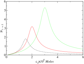
Figure 2: The propagation ratio $\mu_{1\to 3}$ defined in the text in a linear chain $C_{1}\to C_{2}\to C_{3}$ with strong binding ($k=1$nM) as a function of concentration of the intermediate substance $C_{2}$. All curves have the same concentration of the target protein $C_{3}=1\mu$M and different concentrations of the source of the signal $C_{1}=2\mu$M (dashed line), $C_{1}=1\mu$M (solid line), and $C_{1}=0.5\mu$M (dot-dashed line). In the strong binding limit the propagation ratio reaches its maximum when all three substances are completely bound, $C_{2}=C_{1}+C_{3}$. It also follows that the peak propagation is better from high to low total concentration i.e. when $C_{1}>C_{3}$.

In a general case of a PPI network of arbitrary topology the only situation in which free concentrations of all proteins would approach zero as $k_{ij}\to 0$ is when their total concentrations $C_{i}$ are proportional to their degrees $d_{i}$. For a given topology of the network such concentration setup has the slowest decay of perturbations.

Most real-life PPI networks are characterized by a positive correlation between total concentrations of interacting proteins. In the yeast network used in this study we observed this effect to be present and highly statistically significant: (the Spearman rank correlation coefficient of 0.27 with P-value of $10^{-54}$.) Such correlation improves the balance between total concentrations of interacting nodes and thus somewhat lowers the average free concentration of proteins compared to a case where this correlation is absent. Based on this we expect that real protein-protein networks would be more prone to propagating perturbations than their counterparts in which concentrations of proteins are randomly reshuffled and thus the correlation between concentrations of interacting nodes is destroyed. This theoretical expectation was indeed verified in Fig. 1B (compare filled circles and open diamonds for the network with real concentrations and the reshuffled ones).

Most real-life PPI networks are not bipartite. Fortunately, due to a relative sparsity of links the number of odd-length loops in them is small and our resistor network analogy provides a reasonable approximation. For any starting point of perturbation $0$ the optimal way to define sign-alteration in variables $\phi_{i}=(-1)^{x_{i}}\delta F_{i}/F_{i}$ is by using $x_{i}=l_{i0}$ (here $l_{i0}$ is the distance from the source of perturbation $0$ to the node $i$.) The majority of links would connect nodes with opposite ’parities’, while the remaining non-bipartite links could be treated as a small but important correction to the ideal case. Like shunt conductivities to the ground, they contribute to the dissipation of the “current”. Indeed, if a link $i\leftrightarrow j$ is of this anomalous kind, its contribution to the current leaving nodes $i$ and $j$ are equal to each other and given by $D_{ij}(\phi_{i}+\phi_{j})$. One example of such anomalous (non-bipartite) links is given by homodimers (see [3].) In general, these anomalous links lead to the loss of the total current from the system and thus tend to dampen the propagation of perturbations.

In what follows we analytically investigate a simple example of a bipartite network – the Bethe lattice – where all dissociation constants are the same, $k_{ij}=k$, and each vertex has the same number of interaction partners (degree) $d_{i}=d$. When total concentrations of all proteins are also identical $C_{i}=C$, their equilibrium free concentrations are given by

$$F_{i}=F=\frac{k}{2d}\left(\sqrt{1+\frac{4dC}{k}}-1\right).$$ (10)

Small deviations $\delta F_{l}$ at distance $l$ from the perturbation source at node $0$ should satisfy the Eq. (6), which in this case could be rewritten as

$$-(d+\frac{k}{F})\delta F_{l}=(d-1)\delta F_{l+1}+\delta F_{l-1}\qquad.$$ (11)

This equation has an exponentially decaying solution $\delta F_{l}=\delta F_{0}\;\lambda^{l}$, where

$$\lambda=-\frac{1}{d-1}\left(\frac{d+k/F}{2}-\sqrt{\left(\frac{d+k/F}{2}\right)^{2}-(d-1)}\right).$$ (12)

As expected, $-1<\lambda<0$ which means that perturbations sign alternate and exponentially decay as a function of $l$. In a strong binding limit the combination of Eqs. (12,10) yields

$$\lambda=-\frac{1}{d-1}\left(1-\frac{1}{d-2}\sqrt{\frac{dk}{C}}\right)+{\cal O}(\frac{dk}{C}),\qquad.$$ (13)

For a linear chain of proteins ($d=2$), the complete solution in terms of $C$ and $k$ looks particularly elegant:

$$\lambda_{L}=-\frac{(1+8C/k)^{1/4}-1}{(1+8C/k)^{1/4}+1}.$$ (14)

In the limit of strong binding, a perturbation in a linear chain propagates indefinitely, $|\lambda_{1D}|\rightarrow 1$. Using this approach, it also turns possible to find the exact solution for the decay exponent in the linear chain ($d=2$) with oscillating total concentrations of proteins: $C_{i}=C[1+(-1)^{i}a]$. Response of the even- and odd-numbered vertices has different amplitudes yet decays with the same exponential coefficient $\lambda_{\pm}=-[4\chi\sqrt{1-a^{2}}-\sqrt{2f(1+4\chi)-2f^{2}}]/[1+4\chi-f],$ where $\chi=C/k$ and $f=\sqrt{16a^{2}\chi^{2}+8\chi+1}$. Evidently, $|\lambda_{\pm}(C/k,a)|\leq\lambda_{L}(C/k)$ with equality being achieved only for $a=0$. Thus, as was argued in a general case, any variation in $C_{i}/d_{i}$ results in a larger average unbound concentrations $F_{i}$ and thus in a faster decay of perturbations.

This work was supported by 1 R01 GM068954-01 grant from the NIGMS. Work at Brookhaven National Laboratory was carried out under Contract No. DE-AC02-98CH10886, Division of Material Science, U.S. Department of Energy. Work at the NBI was supported by the Danish National Research Foundation. II and KS thank Theory Institute for Strongly Correlated and Complex Systems at BNL for financial support during their visits.

References

- [1] D. B. Shear, J. Chem. Phys., 48, 4144 (1968).
- [2] S. Maslov and I. Ispolatov, in preparation.
- [3] Above we implicitly assumed that every protein enters every dimer in one copy. That is obviously not true for homodimers (as well as possibly for some heterodimers). For proteins forming homodimers the conservation law 2 changes to and thus the diagonal term is given by .
- [4] C. Stark, B.-J. Breitkreutz, T. Reguly,L. Boucher,A. Breitkreutz, and M. Tyers, Nucl. Acids Res. 34, D535 (2006).
- [5] S. Ghaemmaghami, W.-K. Huh, K. Bower, R.W. Howson, A. Belle, N. Dephoure, E.K. O’Shea, and J. S. Weissman, Nature, 425, 737 (2003).
- [6] J.R.S. Newman, S. Ghaemmaghami, J. Ihmels, J., D. K. Breslow, M. Noble, J. L. DeRisi, and J.S Weissman, Nature, 441, 840 (2006).