Phylogenetic tree constructing algorithms fit for grid computing with SVD

Abstract.

Erikkson showed that singular value decomposition(SVD) of flattenings determined a partition of a phylogenetic tree to be a split ([7]). In this paper, based on his work, we develop new statistically consistent algorithms fit for grid computing to construct a phylogenetic tree by computing SVD of flattenings with the small fixed number of rows.

1. Introduction

Phylogenetic analysis of a family of related nucleic acid or protein sequences is to determine how the family could have been derived during evolution. Assume that evolution follows a tree model with evolution acting independently at different sites of genome. Let the transition matrices for this model be the general Markov model which is more general than any other in the Felsenstein hierarchy. How to reconstruct evolutionary trees is one of the main objects in phylogenetics.

Since statistical models are algebraic varieties, we are interested in defining polynomials called phylogenetic invariants for varieties. Many authors have studied phylogenetic invariants for different models ([1], [4], [9], [13], [16]). Phylogenetic invariants have been used for phylogenetic tree reconstruction ([5]).

Procedures for phylogenetic analysis are linked to those for sequence alignment. We can easily organize a group of similar sequences with a small variation into a phylogenetic tree. On the other hand, as sequences become more different through evolutionary change, as they can be more difficult to be aligned. A phylogenetic analysis of very different sequences is also hard to do since there are many possible evolutionary paths that could have been followed to produce the observed sequence variation. To solve these difficulties and complexities many phylogenetic analysis programs have been invented. The main ones in use are PHYLIP (phylogenetic inference package, [8]) available from Dr. J. Felsestein and PAUP ([17]) available from Sinauer Associates, Sunderland, Massachusetts. Nowadays these programs provide three methods for phylogenetic analysis - Parsimony, distance, and maximum likelihood methods - and also give many evolutionary models for sequence variation.

Note that splits in a phylogenetic tree play an important role in reconstructing the phylogenetic tree ([15]). Recall that Erikkson suggested a phylogenetic tree building algorithm using SVD of flattenings in Chapter 19 ([7]) of [10]. In that article, he tried to build a phylogenetic tree without concerning the notion of distance by concentrating on the phylogenetic invariants which are given by rank conditions of flattenings. On the other hand, he had difficulty in dealing with the phylogenetic tree having a large number of leaves since he had to compute SVD of flattenings of huge size. In this paper, we construct algorithms with SVD of flattenings of fixed number of rows, i.e., 16. We will present tree building algorithms (Algorithm 1 and Algorithm 2) in section 3,4 using SVD to calculate how close a matrix is to be a certain rank. In section 5, we use the program seq-gen ([12]) to simulate data of various lengths for the phylogenetic tree. After that we build a phylogenetic tree using Algorithm 1, Algorithm 2 and Neighbor joining algorithm (NJ). It turns out that our algorithms are efficient to construct the phylogenetic tree involving $n\geq 15$ species for DNA sequences with respect to the numerical stability. Also we compare our algorithms to NJ using simulated and real Encode data. Our algorithms are suitable to construct phylogenetic trees for general Markov models, i.e. models coming from real data.

Acknowledgements

We would like to thank Lior Pachter, Bernd Sturmfels and Seth Sullivant for discussing tree building algorithm and encouraging us to write this paper. Also first author thanks organizers and participants of Summer school “Algebraic statistics, Tropical geometry, Computational biology” in Norway for warm hospitality and helpful discussion about these areas during he attended in the school.

2. Notations and Preliminaries

In this section we explain known results by Erikkson and basic concepts in the book: Algebraic statistics for computational biology ([10]) for the later use. We will present basic theorem which plays an important role in this paper.

A phylogenetic $X$-tree $T$ is a tree with leaf set $X$ and no vertices of degree two. If every interior vertex of a $X$-tree has degree three, then $T$ is called a trivalent tree. A split $A|B$ of $X$ in a tree $T$ is a partition of the leaves into two non-empty blocks, $A$ and $B$. Removing an edge $e$ from a phylogenetic $X$-tree $T$ divides $T$ into two connected components, which induces a split of the leaf set $X$. We will call this the split associated with $e$. The collection of all the splits associated with the edges of $T$ is called the splits of $T$ denoted by $\mathcal{S}(T)$. Two splits $A_{1}|B_{1}$ and $A_{2}|B_{2}$ of $X$ are compatible if at least one of the four intersections $A_{1}\cap A_{2},A_{1}\cap B_{2},B_{1}\cap A_{2},$ and $B_{1}\cap B_{2}$ is empty. Also note that a collection $\mathcal{S}$ of splits of $X$ is compatible if it is contained in the splits of some tree $T$ ([2]). We adopt all of these notations in [3].

Theorem 2.1 ([10]).

A collection $\mathcal{S}$ of splits of $X$ is pairwise compatible if and only if there exists a tree $T$ such that $\mathcal{S}=\mathcal{S}(T)$.

Let $X=[n]:=\{1,\cdots,n\}$ and $m$ be the number of states in the alphabet,

$$m=|\Sigma|=\begin{cases}2,\quad\Sigma=\{0,1\}\\ 4,\quad\Sigma=\{A,C,G,T\}.\end{cases}$$

Set $p_{i_{1}\cdots i_{n}}$ is the joint probability that leaf $j$ is observed to be in state $i_{j}$ for all $j\in\{1,\cdots,n\}$. Write $P$ for the entire probability distribution.

Definition 2.2.

A flattening along a partition $A|B$ is the $m^{|A|}$ by $m^{|B|}$ matrix where the rows are indexed by the possible states for the leaves in $A$ and the columns are indexed by the possible states for the leaves in $B$. The entries of this matrix are given by the joint probabilities of observing the given pattern at the leaves. We write $\mbox{Flat}_{A|B}(P)$ or shortly $F_{A|B}(P)$ for this matrix.

Next we define a measurement that a general partition of the leaves is close to a split. If $A$ is a subset of the leaves of $T$, then let $T_{A}$ be the subtree induced by the leaves in $A$. That is, $T_{A}$ is the minimal set of edges needed to connect the leaves in $A$.

Definition 2.3.

Suppose that $A|B$ is a partition of $[n]$. The distance between the partition $A|B$ and the nearest split, written $e(A,B)$, is the number of edges that occur in $T_{A}\cap T_{B}$.

Notice that $e(A,B)=0$ exactly when $A|B$ is a split. Consider $T_{A}\cap T_{B}$ as a subtree of $T_{A}$. Color the nodes in $T_{A}\cap T_{B}$ red, the nodes in $T_{A}\setminus(T_{A}\cap T_{B})$ blue. Say that a node is monochromatic if it and all of its neighbors are of the same color. We let $\text{mono}(A)$ be the number of monochromatic red nodes.

Definition 2.4.

Define $\text{mono}(A)$ as the number of nodes in $T_{A}\cap T_{B}$ that do not have a node in $T_{A}\setminus(T_{A}\cap T_{B})$ as a neighbor.

The following theorem shows how close a partition is to being a split with the rank of the flattening associated to that partition. Originally this theorem is proved for the case that $T$ is a trivalent tree. On the other hand, we have the same result for the non-trivalent tree $T$ whose proof is almost same as original one in [7].

Theorem 2.5.

Let $A|B$ be a partition of $[n]$, $T$ be an unrooted tree which is not necessarily trivalent with leaves labeled by $[n]$, and assume that the joint probability distribution $P$ comes from a Markov model on $T$ with an alphabet with $m$ letters. Then the generic rank of the flattening $\mbox{F}_{A|B}(P)$ is given by

$$\min(m^{e(A,B)+1-\mbox{mono}(A)},m^{e(A,B)+1-\mbox{mono}(B)},m^{|A|},m^{|B|}).$$

Proof.

Refer to [7], Theorem 19.5. ∎

Using Theorem 2.5 we have the following corollaries.

Corollary 2.6.

If $A|B$ is a split in the tree, the generic rank of $F_{A|B}(P)$ is m.

Corollary 2.7.

If $A|B$ is not a split in a trivalent tree and we have $|A|,|B|\geq 2$ then the generic rank of $\mbox{F}_{A|B}(P)$ is at least $m^{2}$.

For the non-trivalent tree case we have a different result comparing to Corollary 2.7, i.e., generic rank of ${F}_{A|B}(P)$ is at least $m$. The reason for the different result comes from considering the following 4-valent tree with $A=\{1,2\},B=\{3,4,5,6,7,8\}$. Actually, in this case we have $R=\{v_{1}\}$, $e(A,B)+1-\mbox{momo}(A)=1,e(A,B)+1-\mbox{momo}(B)=1$ for non-split $A|B$. Hence we get $\mbox{rank}F_{A|B}(P)=m$.

Figure 1. Non-trivalent tree

A singular value decomposition of a $m\times n$ matrix $A$ (with $m\geq n$) is a factorization $A=U\Sigma V^{T}$ where $U$ is $m\times n$ and satisfies $U^{T}U=I$, $V$ is $n\times n$ and satisfies $V^{T}V=I$ and $\Sigma=\mbox{diag}(\sigma_{1},\sigma_{2},\cdots,\sigma_{n})$, where $\sigma_{1}\geq\sigma_{2}\geq\cdots\geq\sigma_{n}\geq 0$ are called the singular values of $A$.

We need the following theorem to define svd distance in the next section.

Theorem 2.8 ([6], Theorem 3.3).

The distance from $A$ to the nearest rank $k$ matrix is $\displaystyle\min_{\mbox{rank}(B)=k}\|A-B\|_{F}=\sqrt{\sum^{n}_{i=k+1}\sigma^{2}_{i}}$ in the Frobenius norm.

3. Algorithm for constructing a phylogenetic tree

In this section, we have an algorithm for constructing a phylogenetic tree using SVD of flattenings which improves Erikkson’s algorithm in view of numerical stability (cf. [7]). First we define a function called svd-cherry as follows.

Definition 3.1.

For each distinct pair $(s_{i},s_{j})$ in the $k$ species $\mathcal{S}_{k}=\{s_{1},s_{2},\cdots,s_{k}\}$, svd distance $d_{F}(s_{i},s_{j},\mathcal{S}_{k})$ between $s_{i}$, and $s_{j}$ in $\mathcal{S}_{k}$ is defined by the distance from the flattening $F_{\{s_{i},s_{j}\}|\{s_{1},\cdots,s_{k}\}\backslash\{s_{i},s_{j}\}}(P)$ to the nearest rank $m$ matrix in the Frobenius norm.

Definition 3.2.

For given $k$ species $\mathcal{S}_{k}=\{s_{1},s_{2},\cdots,s_{k}\}$, Define

$$\text{\rm svd-cherry}(s_{1},s_{2},\cdots,s_{k}):=(s_{i^{*}},s_{j^{*}},v)$$

so that the pair $(s_{i^{*}},s_{j^{*}})$ in $\mathcal{S}_{k}$ and their svd distance $v$ in $\mathcal{S}_{k}$ satisfies that

$$v:=d_{F}(s_{i^{*}},s_{j^{*}},\mathcal{S}_{k})=\displaystyle\min\{d_{F}(s_{i},s_{j},\mathcal{S}_{k})~{}|~{}(i,j)\\ \in[k]\times[k],~{}i\neq j\}.$$

Using Definition 3.2, we have the following algorithm.

Algorithm 1 (Building a phylogenetic tree using SVD of flattenings)

Input: A multiple alignment of genomic data from $n$ species from the alphabet $\Sigma$ with $m$ states.

Output: An unrooted phylogenetic tree $T$ with $n$ leaves labeled by the species.

Initialization: Partition $n$ species $s_{1},s_{2},\cdots,s_{n}$ into $n$ singletons as $C_{1,1},C_{1,2},\cdots,C_{1,n}$.

Loop: For $k$ from $1$ to $n-3$, perform the following steps.

Step 1: For each $n-k+1$ species $s_{1},s_{2},\cdots,s_{n-k+1}$ where $s_{l}\in C_{k,l}$ is a representative of $C_{k,l}$, $1\leq l\leq n-k+1$, find a distinct pair of clusters $(C_{k,i^{*}},C_{k,j^{*}})$ such that $\text{\rm svd-cherry}(s_{1},s_{2},\cdots,s_{n-k+1}):=(s_{i^{*}},s_{j^{*}},v)$ for $s_{i^{*}}\in C_{k,i^{*}},s_{j^{*}}\in C_{k,j^{*}}$.

Step 2: Choose the pair of clusters $(C_{k,i^{\diamond}},C_{k,j^{\diamond}})$ which occurs most frequently in Step 1.

Step 3: Join $C_{k,{i^{\diamond}}}$ and $C_{k,{j^{\diamond}}}$ together in the tree and consider this as a new cluster $C_{k+1,1}$. After that rename the remaining $C_{k,l}$’s as $C_{k+1,2},\cdots,C_{k+1,n-k}$.

Proposition 3.3.

Algorithm 1 needs to compute SVD at most $\sum^{n}_{k=4}[(\frac{n}{k})^{k}]{k\choose 2}$ times. Here $[(\frac{n}{k})^{k}]$ is the maximum possible integer not greater than $(\frac{n}{k})^{k}$.

Proof.

If we have $k$ clusters $C_{1},C_{2},\cdots,C_{k}$, then the number of possible representatives for each clusters is $\prod^{k}_{1}|C_{i}|$. Since $\sum^{k}_{1}|C_{i}|=n,$ $\prod^{k}_{1}|C_{i}|$ has maximum $(\frac{n}{k})^{k}$ where $|C_{1}|=|C_{2}|=\cdots=|C_{k}|=\frac{n}{k}$. Here $|C_{i}|$ is the cardinality of $C_{i}$. Thus we manipulate SVD at most $\sum^{n}_{k=4}[(\frac{n}{k})^{k}]{k\choose 2}$ times in total for the flattenings with fixed number of rows, i.e., $m^{2}$. ∎

Each cluster $C_{k,l},~{}1\leq k\leq n-2,~{}1\leq l<n-k+1$ in Algorithm 1 means a split in the tree. In Algorithm 1 we have the following hierarchy of $C_{k,l}$’s. In the Initialization, $C_{1,l}~{}(1\leq l\leq n)$ mean $n$ trivial splits, in other words, outer edges in tree $T$. At the end of the first loop, there is one new cluster among $C_{2,l}~{}(1\leq l\leq n-1$), which means one new split in $T$. At the end of each $k$-th loop from $k=1$ up to $k=n-3$, we obtain one new edge in $T$. In total we have the exact $2n-3$ splits in $T$.

$$k=1:~{}~{}\quad\qquad\qquad~{}~{}~{}C_{1,1}~{}~{}C_{1,2}~{}~{}C_{1,3}~{}~{}\cdots\cdots\cdots~{}~{}C_{1,n-2}~{}~{}C_{1,n-1}~{}~{}C_{1,n}$$

$$k=2:~{}~{}\quad\qquad\qquad~{}~{}~{}C_{2,1}~{}~{}C_{2,2}~{}~{}C_{2,3}~{}~{}\cdots\cdots\cdots~{}~{}C_{2,n-2}~{}~{}C_{2,n-1}$$

$$k=3:~{}~{}\quad\qquad\qquad~{}~{}~{}C_{3,1}~{}~{}C_{3,2}~{}~{}C_{3,3}~{}~{}\cdots\cdots\cdots~{}~{}C_{3,n-2}$$

$$\qquad\quad\quad\qquad\qquad\vdots\qquad\vdots\qquad\vdots\qquad\vdots~{}~{}$$

$$k=n-3:\quad\quad C_{n-3,1}~{}~{}C_{n-3,2}~{}~{}C_{n-3,3}~{}~{}C_{n-3,4}$$

$$k=n-2:\quad\quad C_{n-2,1}~{}~{}C_{n-2,2}~{}~{}C_{n-2,3}$$

The matrix size $m^{2}\times m^{k-2}$ of flattenings may be large where $k$ varies from $n$ to 4, on the other hand flattenings are very sparse. Thus, it is faster to compute the eigenvalues of $A^{T}A$ of fixed size $m^{2}\times m^{2}$ for every flattening $A$ than singular values of $A$ itself of size $m^{2}\times m^{k-2}$. Erikkson computed singular values of flattenings of various huge size $m^{|A|}\times m^{|B|}$ where $A|B$ is a partition of $[n]$. That must cause numerical instability. We, however, avoid computational difficulties which come from numerical instability since we only deal with $A^{T}A$ of fixed size $m^{2}\times m^{2}$ for every flattening $A$. Although we also have difficulty in computing lots of SVD of matrices of fixed size $m^{2}\times m^{2}$, if the number of species grows, Algorithm 1 is fit for parallel computing, especially, grid computing which arranges lots of volunteer computing resources to do distributed computing.

Theorem 3.4.

Algorithm 1 is statistically consistent.

Proof.

By Corollary 2.6, we can see that $d_{F}(s_{i},s_{j},\mathcal{S}_{k})$ goes to 0 if $\{s_{i},s_{j}\}|\{s_{1},\cdots,s_{k}\}\\ \backslash\{s_{i},s_{j}\}$ is a true split of $\mathcal{S}_{k}=\{s_{1},\cdots,s_{k}\}$. While Corollary 2.7 shows that $d_{F}(s_{i},s_{j},\mathcal{S}_{k})$ does not go to 0 if $\{s_{i},s_{j}\}|\{s_{1},\cdots,s_{k}\}\backslash\{s_{i},s_{j}\}$ is a partition which is not a split of $\mathcal{S}_{k}$. Hence, as the empirical distribution approaches the true one, the distance of a split from rank $m$ will go to zero while the distance from rank $m$ of a non-split will not. Therefore Algorithm 1 picks a correct split at each loop. ∎

Figure 2. Model tree for 6 species.

Example

We begin with an alignment of DNA data of length 1000 for 6 species, labeled $1,\cdots,6,$ simulated from the tree in Figure 2 with all branch lengths equal to 0.1. For the loop ($k=1$), let $C_{1,1}=\{1\},C_{1,2}=\{2\},C_{1,3}=\{3\},C_{1,4}=\{4\},C_{1,5}=\{5\},C_{1,6}=\{6\}$ and consider all pairs of the 6 species. In the following results, the svd-val($s_{1},s_{2}|s_{3},\cdots,s_{k}$) is the distance from the flattening $F_{\{s_{1},s_{2}\}|\{s_{3},\cdots,s_{k}\}}(P)$ to the nearest rank $4$ matrix in the Frobenius norm as in Theorem 2.8

loop: k = 1

svd-val( 1, 2 | 3, 4, 5, 6 ) = 0.0188

svd-val( 1, 3 | 2, 4, 5, 6 ) = 0.2102

svd-val( 1, 4 | 2, 3, 5, 6 ) = 0.2103

svd-val( 1, 5 | 2, 3, 4, 6 ) = 0.4297

svd-val( 1, 6 | 2, 3, 4, 5 ) = 0.4298

svd-val( 2, 3 | 1, 4, 5, 6 ) = 0.2095

svd-val( 2, 4 | 1, 3, 5, 6 ) = 0.2096

svd-val( 2, 5 | 1, 3, 4, 6 ) = 0.4298

svd-val( 2, 6 | 1, 3, 4, 5 ) = 0.4297

svd-val( 3, 4 | 1, 2, 5, 6 ) = 0.0128

svd-val( 3, 5 | 1, 2, 4, 6 ) = 0.4779

svd-val( 3, 6 | 1, 2, 4, 5 ) = 0.4779

svd-val( 4, 5 | 1, 2, 3, 6 ) = 0.4779

svd-val( 4, 6 | 1, 2, 3, 5 ) = 0.4779

svd-val( 5, 6 | 1, 2, 3, 4 ) = 0.0076

min value cherry = ( 5, 6 )

After first loop, since svd-cherry($1,2,3,4,5,6$)=(5, 6, 0.0076), we have a new cluster $C_{2,1}=\{5,6\}$ and rename $C_{2,2}=\{1\},C_{2,3}=\{2\},C_{2,4}=\{3\},C_{2,5}=\{4\}$.

loop: k = 2

svd-val( 1, 2 | 3, 4, 5 ) = 0.0216

svd-val( 1, 3 | 2, 4, 5 ) = 0.2104

svd-val( 1, 4 | 2, 3, 5 ) = 0.2105

svd-val( 1, 5 | 2, 3, 4 ) = 0.0214

svd-val( 2, 3 | 1, 4, 5 ) = 0.2094

svd-val( 2, 4 | 1, 3, 5 ) = 0.2095

svd-val( 2, 5 | 1, 3, 4 ) = 0.0290

svd-val( 3, 4 | 1, 2, 5 ) = 0.0127

svd-val( 3, 5 | 1, 2, 4 ) = 0.2101

svd-val( 4, 5 | 1, 2, 3 ) = 0.2099

min value cherry = ( 3, 4 )

--------------------------------------------------

svd-val( 1, 2 | 3, 4, 6 ) = 0.0169

svd-val( 1, 3 | 2, 4, 6 ) = 0.2090

svd-val( 1, 4 | 2, 3, 6 ) = 0.2091

svd-val( 1, 6 | 2, 3, 4 ) = 0.0213

svd-val( 2, 3 | 1, 4, 6 ) = 0.2084

svd-val( 2, 4 | 1, 3, 6 ) = 0.2085

svd-val( 2, 6 | 1, 3, 4 ) = 0.0257

svd-val( 3, 4 | 1, 2, 6 ) = 0.0127

svd-val( 3, 6 | 1, 2, 4 ) = 0.2090

svd-val( 4, 6 | 1, 2, 3 ) = 0.2089

min value cherry=( 3, 4 )

For the loop ($k=2$), first take 5 as a representative of $C_{2,1}=\{5,6\}$ and get svd-cherry($1,2,3,4,5$) =(3, 4, 0.0127). Next choose 6 as a representative of $C_{2,1}=\{5,6\}$ and get svd-cherry($1,2,3,4,6$) =(3, 4, 0.0127). Most frequent pair of clusters in $C_{2,1},\cdots,C_{2,5}$ is $(C_{2,4},C_{2,5})$. We obtain a new cluster $C_{3,1}=\{3,4\}$ and rename $C_{3,2}=\{5,6\},~{}C_{3,3}=\{1\},~{}C_{3,4}=\{2\}$.

loop: k = 3

svd-val( 1, 2 | 5, 3 ) = 0.0213

svd-val( 1, 5 | 2, 3 ) = 0.0208

svd-val( 1, 3 | 2, 5 ) = 0.0285

min value cherry=( 1, 5 )

--------------------------------------------------

svd-val( 1, 2 | 6, 3 ) = 0.0167

svd-val( 1, 6 | 2, 3 ) = 0.0207

svd-val( 1, 3 | 2, 6 ) = 0.0252

min value cherry=( 1, 2 )

--------------------------------------------------

svd-val( 1, 2 | 5, 4 ) = 0.0214

svd-val( 1, 5 | 2, 4 ) = 0.0221

svd-val( 1, 4 | 2, 5 ) = 0.0295

min value cherry=( 1, 2 )

--------------------------------------------------

svd-val( 1, 2 | 6, 4 ) = 0.0168

svd-val( 1, 6 | 2, 4 ) = 0.0219

svd-val( 1, 4 | 2, 6 ) = 0.0262

min value cherry=( 1, 2 )

For the loop ($k=3$), first take 3 as a representative of $C_{3,1}=\{3,4\}$, 5 as a representative of $C_{3,2}=\{5,6\}$, then we get svd-cherry($3,5,1,2$)=(1, 5, 0.0208). Next choose 3 as a representative of $C_{3,1}=\{3,4\}$, 6 as a representative of $C_{3,2}=\{5,6\}$, get svd-cherry($3,6,1,2$)=(1, 2, 0.0167). By the same manner we have svd-cherry($5,4,1,2$)=(1, 2, 0.0214), svd-cherry($6,4,1,2$)=(1, 2, 0.0168). Most frequent pair of clusters in $C_{3,1},\cdots,C_{3,4}$ is $(C_{3,3},C_{3,4})$. We obtain a new cluster $C_{4,1}=\{1,2\}$ and rename $C_{4,2}=\{5,6\},~{}C_{4,3}=\{3,4\}$. We can join these three clusters $C_{4,1},C_{4,2},C_{4,3}$ to make an unrooted tree.

4. Simplified tree constructing algorithm

In Algorithm 1, if we can reduce the number of feasible representative of each cluster $C_{k,l}$ using some available a priori information, then computational cost can be saved. In this section, for example, we choose the unique feasible representative of each cluster which has the smallest distance from species outside the cluster.

Algorithm 2 (Simplified tree constructing algorithm)

Input: A multiple alignment of genomic data from $n$ species from the alphabet $\Sigma$ with $m$ states.

Output: An unrooted phylogenetic tree $T$ with $n$ leaves labeled by the species.

Initialization: Partition $n$ species $s_{1},s_{2},\cdots,s_{n}$ into $n$ singletons as $C_{1,1},C_{1,2},\cdots,C_{1,n}$.

Loop: For $k$ from $1$ to $n-3$, perform the following steps.

Step 1: For each cluster $C_{k,j},~{}1\leq j\leq n-k+1$, choose the representative $s_{j}^{R}\in C_{k,j}$ by the following;

For all $s\in C_{k,j}$, calculate $v_{s}={\sum_{s^{\prime}\in[n]\backslash C_{k,j}}p(s,s^{\prime})}$ where $p(s,s^{\prime})$ is the

proportion of different nucleotides between two species $s,s^{\prime}$. Choose $s_{j}^{R}\in C_{k,j}$

which has the smallest value $v_{s}$ for all $s\in C_{k,j}$.

Step 2: For $(s^{R}_{1},s^{R}_{2},\cdots,s^{R}_{n-k+1})$ where $s^{R}_{l}\in C_{k,l},1\leq l\leq n-k+1$, find a distinct pair of clusters $(C_{k,i^{*}},C_{k,j^{*}})$ such that $\text{\rm svd-cherry}(s_{1}^{R},s_{2}^{R},\cdots,s^{R}_{n-k+1}):=(s_{i^{*}},s_{j^{*}},v)$ for $s_{i^{*}}\in C_{k,i^{*}},s_{j^{*}}\in C_{k,j^{*}}$.

Step 3: Join $C_{k,{i^{*}}}$ and $C_{k,{j^{*}}}$ together in the tree and consider this as a new cluster $C_{k+1,1}$. After that rename the remaining $C_{k,l}$’s as $C_{k+1,2},\cdots,C_{k+1,n-k}$.

Note that Algorithm 2 is much faster to construct phylogenetic trees with many leaves since it uses only one representative for each cluster $C_{k,l}$.

5. Performance analysis of tree constructing algorithms

5.1. Building phylogenetic trees with simulated data

We chose phylogenetic tree models as in Figure 3 and simulated DNA sequence data on these trees using the program seq-gen ([12]). Figure 3 shows variables $a,b,c$ in the trees. These trees were chosen as difficult trees in [14]. Next, we built trees using Algorithm 1,2 and neighbor joining algorithm with Jukes-Cantor distance from these data, respectively. For each algorithm, we plotted percent of tree reconstructed among 1000 DNA data set for various sequence lengths.

Figure 4 shows the results for the case of $a=.01,b=.04,c=.07$ for both model trees in Figure 3. The results for the case of $a=.02,b=.13,c=.19$ are shown in Figure 5. Algorithm 1 shows better performance than Algorithm 2, but, worse than the neighbor joining algorithm. It might be expected because the used DNA data were simulated by distance based algorithm.

Figure 3. Model trees (A)(left) and (B)(right).

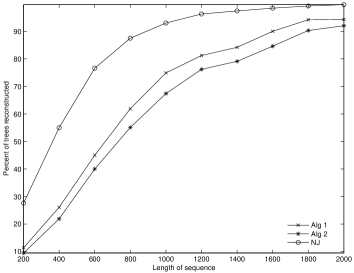
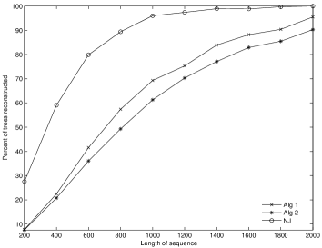
Figure 4. Simulation results of tree construction methods for Model trees A(left) and B(right) in the case $a=.01,~{}b=.04,~{}c=.07$.

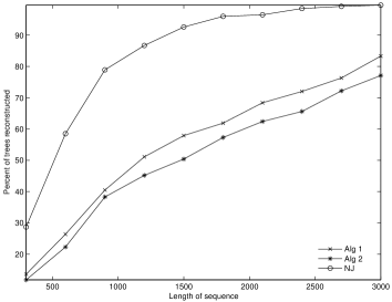
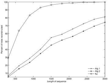
Figure 5. Simulation results of tree construction methods for Model trees A(left) and B(right) in the case $a=.02,~{}b=.13,~{}c=.19$.

Figure 6. Phylogenetic tree with 32 leaves whose all of the edges have branch length .1.

We tested Algorithm 1,2 to reconstruct a tree with many species, for example 32 species. We simulated 100 DNA data sets of length 1000 for 32 species from the tree in Figure 6 with all branch lengths equal to .1. We got 94 % of reconstruction rate using Algorithm 2, whereas 99 % of reconstruction rate with neighbor joining algorithm. For the Algorithm 1, we tested only 1 data set using parallel cluster machine with 10 Athlon 2600 CPUs. It took about 3 hours for 1 data set. The loop number which took longest time was 19. Algorithm 1 did $2^{16}{14\choose 2}$ SVD computations in 19-th loop. The important point is that we change the type of difficulty in dealing with rebuilding tree of many species from time and numerical instability to time only. Furthermore, the difficulty in time can be overcome in various ways.

5.2. Building phylogenetic trees with real data

For data, we use the September 2005 freeze of the ENCODE alignments. We restrict our attention to the problem of constructing phylogenetic tree for 8 species: human, chimp, galago, mouse, rat, cow, dog, and chicken, which is called rodent problem. We processed each of the 44 ENCODE regions to obtain data sets which have ungapped columns greater than 100 bps in length. We obtain 75 data sets in manually chosen 14 Enm regions and 301 data sets in all 44 Encode regions.

Recall that the Robinson-Foulds metric which is also called the partition metric was proposed by [11] is one of the simplest metrics on trees. The distance between two trees $T_{1}$ and $T_{2}$ is defined by

$$d_{RF}(T_{1},T_{2})=\frac{1}{2}(|\mathcal{S}(T_{1})-\mathcal{S}(T_{2})|+|\mathcal{S}(T_{2})-\mathcal{S}(T_{1})|).$$

Here $\mathcal{S}(T)$ is the set of splits in $T$ and $|\mathcal{S}(T_{i})-\mathcal{S}(T_{j})|$ is the cardinality of the set $\mathcal{S}(T_{i})-\mathcal{S}(T_{j})$. The symmetric distance $d_{s}(T_{1},T_{2})$ is twice of $d_{RF}(T_{1},T_{2})$.

Rodents have very different morphological features, although their molecular data is similar to that of the primates. Thus, lots of biologists pay attention to rodents. Tree construction algorithms using genomic data usually misplace the rodents, mouse and rat, on the tree, with respect to other mammals. According to fossil records and molecular data, we have the biologically correct tree that is not sure whether it is correct. In this tree we have the primate clade with human and chimpanzee and then the galago as an outgroup to these two. The rodent clade (mouse and rat) is a sister group to the clade (human, chimpanzee and galago) and the clade (dog and cow) is the outgroup to former 5 species. The chicken is an outgroup to all of these as a root of this phylogenetic tree. On the other hand, usual tree reconstruction algorithm mislocate the rodents and so locate them as an out group to the clade (human, chimpanzee and galago) (See Figure 7).

Figure 7. Biologically correct tree(left) and the tree which is obtained by usual algorithm(right).

method	Algorithm 1	Algorithm 2	NJ
All ($P_{c}$)	11.9	10.6	11.6
All ($d_{s}$)	2.57	2.85	2.77
Enm($P_{c}$)	12.0	12.0	14.6
Enm ($d_{s}$)	2.14	2.52	2.45

Table 1. Comparing results for algorithms on data from Encode project. $P_{c}$ is percent of trees reconstructed and $d_{s}$ is symmetric distance.

The reasons for this are not entirely known, but it could be since tree construction methods generally assume the existence of a global rate matrix for all the species. However, rat and mouse have mutated faster than the other species. Our algorithms does not assume anything about the rate matrix ([10], Chapter 21).

In fact, Table 1 shows that our algorithms performs quite well on the ENCODE data sets comparing to NJ(neighbor joining algorithm with Jukes-Cantor distance) algorithm. Algorithm 1 constructs the correct tree similar to NJ (cf. [7], p.357), but, has shorter symmetric distance $d_{s}$ on average than NJ algorithm.

References

- [1] Allman, ES. and Rhodes, JA., Phylogenetic invariants for the general Markov model of sequence mutation, Mathematical Biosciences, 186(2): 113-144, 2003.
- [2] Buneman, P., The recovery of trees from measures of dissimilarity, Mathematics in the Archaeological and Historical Sciences, Edinburgh University Press, 387-395, 1971.
- [3] Bryant, D., The Splits in the Neighborhood of a Tree, Annals of Combinatorics, 8: 1-11, 2004.
- [4] Cavender, J. and Felsenstein, J., Invariants of phylogenies in a simple case with discrete states, Journal of Classification, 4:57-71, 1987.
- [5] Casanellas, M. and Fernandez, J. Efficiency of a new phylogenetic reconstruction method based on invariants, preprint, 2006.
- [6] Demmel, JW., Applied Numerical Linear Algebra, SIAM, 1997.
- [7] Eriksson, N., Tree construction using singular value decomposition, Chapter 19, Algebraic statistics for computational biology, Cambrige University Press, 2005.
- [8] Felsenstein, J., PHYLIP, Phylogeny Inference Package Version 3.6 distributed by the author: http://evolution.genetics.washington.edu/phylip. html, Department of Genomic Sciences University of Washington, Seattle, 2004.
- [9] Lake, JA., A rate dependent technique for analysis of nucleic acid sequences: evolutionary parsimony, Molecular Biology and Evolution, 4;167-191, 1987.
- [10] Patchter, L. and Sturmfels, B., Algebraic statistics for computational biology, Cambrige University Press, 2005.
- [11] Robinson, DF. and Foulds, LR., Comparison of weighted labelled trees, Combinatorial Mathematics, VI, Proc. Sixth Austral. Conf., Lecture Notes in Mathematics, Vol 748, Springer-Verlag, 119-126, 1979.
- [12] Rambaut, A. and Grassly, NC., Seq-gen: An application for the Monte Carlo simulation of DNA sequence evolution along phylogenetic trees, Comput. Appl. Biosci., 13: 235-238, 1997.
- [13] Sankoff, D. and Blanchette N., Comparative genomics via phylogenetic invariants for Jukes-Cantor Semigroups, Proceedings of the International Conference on Stochastic models, American Mathematical Society, 399-418, 2000.
- [14] Saitou, N. and Nei, M., The Neighbor-joining Method: A New Method for Reconstructing Phylogenetic Trees, Molecular Biology and Evolution, 4:406-425, 1987.
- [15] Sturmfels, B., Can biology lead to new theorems?, preprint, 2006.
- [16] Sturmfels, B. and Sullivant, S., Toric ideals of phylogenetic invariants, Journal of Computational Biology, 12: 204-228, 2005.
- [17] Swofford, DL., PAUP. http://www.lms.si.edu/PAUP, Phylogenetic Analysis using Parsimony, Sunderland Mass, 1998.