Heterogeneous Cell Population Dynamics:
Equation-Free Uncertainty Quantification Computations

ABSTRACT

We propose a computational approach to modeling the collective dynamics of populations of coupled heterogeneous biological oscillators. In contrast to Monte Carlo simulation, this approach utilizes generalized Polynomial Chaos (gPC) to represent random properties of the population, thus reducing the dynamics of ensembles of oscillators to dynamics of their (typically significantly fewer) representative gPC coefficients. Equation-Free (EF) methods are employed to efficiently evolve these gPC coefficients in time and compute their coarse-grained stationary state and/or limit cycle solutions, circumventing the derivation of explicit, closed-form evolution equations. Ensemble realizations of the oscillators and their statistics can be readily reconstructed from these gPC coefficients. We apply this methodology to the synchronization of yeast glycolytic oscillators coupled by the membrane exchange of an intracellular metabolite. The heterogeneity consists of a single random parameter, which accounts for glucose influx into a cell, with a Gaussian distribution over the population. Coarse projective integration is used to accelerate the evolution of the population statistics in time. Coarse fixed-point algorithms in conjunction with a Poincaré return map are used to compute oscillatory solutions for the cell population and to quantify their stability.

INTRODUCTION

Autonomous oscillations are observed in biological systems ranging in complexity from microorganisms to human beings (1). Often these oscillations are generated at the cellular level through positive feedback loops embedded in gene regulatory or metabolic networks (2). Robust strategies have evolved, based on intracellular coupling of multiple oscillators (rather than on a single cellular oscillator subject to degradation and failure). A fundamental feature of such multicellular systems is the synchronization of individual oscillators to produce a coherent overall rhythm (3). Synchronized oscillators are responsible for rhythm generation at second (heartbeat generation), daily (circadian timekeeping) and monthly (menstrual cycles) time scales. Malfunctioning of these interconnected oscillators can produce disastrous consequences such as sudden heart attacks and epileptic seizures.

The development of mathematical models to study the synchronization of coupled oscillators has a long and beautiful history (1). Seminal contributions to the fundamental understanding of synchronization have been made by rigorous mathematical analysis of simple model systems (4, 5). The study of mechanistic models of multicellular biological systems typically involves computational approaches such as dynamic simulation and numerical bifurcation analysis. Difficulties in applying such scientific computing tools are largely determined by population model complexity, which in turn is determined by the complexity of the individual cell model and the number of cells included in the population. Certain applications require both a detailed single cell model and a large ensemble of single cells for meaningful computational study. For instance, a single mammalian circadian oscillator contains multiple interconnected feedforward and feedback loops that have been modeled with up to 73 coupled differential equations (6). Meanwhile, the mammalian circadian system is comprised of approximately 10,000 individual oscillators that communicate via neurotransmitter mediated coupling (7). The development of stochastic simulations to generate meaningful population statistics is possible only if the model ensemble size is sufficiently large. Therefore, there is considerable motivation to develop efficient simulation and bifurcation analysis techniques for large, heterogeneous ensembles of coupled, complex biological oscillators. Previous studies of heterogeneity (8, 9) used idealized phase models (a single “phase” equation for each oscillator); in this work, we show how the approach can be applied to ensembles of realistic limit cycle oscillator models.

Among traditional techniques employed in the study of ensemble statistics of stochastic systems, the most popular one is Monte Carlo simulation (10) (or the cell-ensemble method (11) in the biological context). This approach, however, becomes extremely time-consuming when the number of simulation realizations is large, as in the case of multicellular coupled oscillator populations. As an alternative, the stochastic Galerkin method for uncertainty quantification (UQ) has been widely used in recent years for solving stochastic ODEs or PDEs. Pioneering work along these lines (12) studied stochastic systems with Gaussian random variables: by viewing randomness as an additional dimension, beyond the space and time dimensions, the dependence of system responses on random parameters is represented in terms of orthogonal polynomial expansions of random variables. In this context (see Appendix A) all orthogonal polynomials of a given order are called Polynomial Chaoses or Homogeneous Chaoses of that order; projections of the system responses onto the Polynomial Chaos (PC) coefficients evolve deterministically, and equations for their evolution can in principle be obtained, and then solved, by applying a Galerkin projection. The method has been applied for uncertainty quantification purposes in various physical and engineering systems including structures with random properties (12), porous media (13), fluid dynamics (14) and chemical reactions (15). In (16), the method was extended: generalized Polynomial Chaos (gPC), applicable to a variety of continuous and discrete probability measures, was proposed based on the Askey scheme. In addition to representations of orthogonal polynomials, this method was also improved in other directions, in the form of piecewise (h-refinement) representations (17) and wavelet expansions (18).

One advantage of the stochastic Galerkin method, as compared to direct Monte Carlo simulation, is that it can reduce a stochastic system to a deterministic one with (often significantly) fewer degrees of freedom, thus accelerating computation and saving data storage space. In order to apply the stochastic Galerkin method, however, one must derive equations for the temporal evolution of gPC coefficients either explicitly or through a pseudospectral approach (e.g. (19)) and develop a new code for the solution of these equations. To circumvent this additional effort, Equation-Free (EF) methods (20, 21, 22) have been utilized recently to quantify propagation of uncertainty in a stochastic system by evolving gPC coefficients of random solutions using the system dynamic simulator in a nonintrusive way, that is, without deriving the corresponding explicit gPC evolution equations (23). Within this multiscale equation-free framework, the original stochastic dynamics code is viewed as a fine-level simulator, while the (unavailable) ODEs for the time-evolution of the gPC coefficients are viewed as a coarse-grained system model. These equation-free algorithms are built based on protocols that enable communication between different levels of system description; the lifting protocol translates coarse-grained initial conditions to one or more consistent fine scale initial conditions; the restriction protocol computes the coarse-grained description (values of the coarse variables, “observables”) of fine scale system configurations. The success of this class of methods relies on the assumption that closed evolution equations for the dominant (low-order) gPC coefficients exist in principle, even if they are not explicitly available.

The purpose of this paper is to demonstrate that efficient simulation strategies for large populations of coupled biological oscillators can be developed by utilizing these equation-free uncertainty quantification (EF-UQ) based methods. A six-dimensional cellular model of yeast glycolytic oscillations (24, 25) is used to study synchronization of 1,000 heterogeneous cells in a well mixed environment. The random variable (which characterizes the cell population heterogeneity) is chosen as the glucose influx for each cell. In the context of EF-UQ, we demonstrate coarse projective integration, which accelerates temporal simulation of the cell population dynamics, and coarse fixed-point computation combined with Poincaré return maps to efficiently converge on limit cycle solutions, corresponding to synchronous population oscillations. Limits of the applicability of the procedure are discussed, including an extension of the basic methodology to handle loss of synchronization when isolated outlier cells “detach” from the main coherent population and develop individual oscillatory characteristics.

A MECHANISTIC SYNCHRONIZATION MODEL FOR YEAST GLYCOLYTIC OSCILLATIONS

The yeast Saccharomyces cerevisiae exhibits autonomous oscillations with a period of approximately one minute when grown under anaerobic conditions (26, 27, 28). Similar oscillations have been observed in other yeast strains (29, 30) as well as algae (31), muscle (32), heart (33) and tumor (34) cells. Yeast studies suggest that an autocatalytic reaction involving the glycolytic enzyme phosphofructokinase is the main cause of oscillations at the single cell level. Therefore, the observed limit cycle behavior has been termed glycolytic oscillations. Additional experimental work has focused on characterizing the intercellular mechanisms involved in the synchronization of individual yeast cell oscillations (35). Typically, oscillations at the cell population level are observed by continuous monitoring of the average intracellular NADH concentration using fluorometry. Experiments with Saccharomyces cerevisiae grown in anaerobic stirred cuvettes suggest that secreted acetaldehyde is the key signaling molecule in the synchronization mechanism (36, 37).

A number of simple cell models have been developed to capture the glycolytic oscillation mechanism in yeast (38, 39, 40, 41). Cell models based on more detailed descriptions of the glycolytic reaction pathway also have been proposed (42, 43). Small ensembles of single cell models have been used to investigate the synchronization phenomenon (38, 41, 43). In this paper, we use a single cell model of intermediate complexity (25) to demonstrate our computational framework for simulating large populations of coupled biological oscillators. Our cell ensemble model is based on an intracellular coupling mechanism involving the transport of acetaldehyde across the cell membrane (24, 25).

A single cell in the population is described by the following differential equations:

$$\!\!\!\!\!\!\!\!\!\frac{dS_{1,i}}{dt}\!\!\! = \!\!\!J_{0,i}-v_{1,i}=J_{0,i}-k_{1}S_{1,i}A_{3,i}\left[1+\left(\frac{A_{3,i}}{K_{I}}\right)^{q}\right]^{-1}$$ (1)

$$\!\!\!\!\!\!\!\!\!\frac{dS_{2,i}}{dt}\!\!\! = \!\!\!2v_{1,i}-v_{2,i}-v_{6,i}=2k_{1}S_{1,i}A_{3,i}\left[1+\left(\frac{A_{3,i}}{K_{I}}\right)^{q}\right]^{-1}-k_{2}S_{2,i}(N-N_{2,i})-k_{6}S_{2,i}N_{2,i}$$ (2)

$$\!\!\!\!\!\!\!\!\!\frac{dS_{3,i}}{dt}\!\!\! = \!\!\!v_{2,i}-v_{3,i}=k_{2}S_{2,i}(N-N_{2,i})-k_{3}S_{3,i}(A-A_{3,i})$$ (3)

$$\!\!\!\!\!\!\!\!\!\frac{dS_{4,i}}{dt}\!\!\! = \!\!\!v_{3,i}-v_{4,i}-J_{i}=k_{3}S_{3,i}(A-A_{3,i})-k_{4}S_{4,i}N_{2,i}-J_{i}$$ (4)

$$\!\!\!\!\!\!\!\!\!\frac{dN_{2,i}}{dt}\!\!\! = \!\!\!v_{2,i}-v_{4,i}-v_{6,i}=k_{2}S_{2,i}(N-N_{2,i})-k_{4}S_{4,i}N_{2,i}-k_{6}S_{2,i}N_{2,i}$$ (5)

$$\!\!\!\!\!\!\!\!\!\frac{dA_{3,i}}{dt}\!\!\! = \!\!\!-2v_{1,i}+2v_{3,i}-v_{5,i}=-2k_{1}S_{1,i}A_{3,i}\left[1+\left(\frac{A_{3,i}}{K_{I}}\right)^{q}\right]^{-1}+2k_{3}S_{3,i}(A-A_{3,i})-k_{5}A_{3,i}$$ (6)

where the index $i$ denotes the cell. The pathway model accounts for glucose flux into the cell ($J_{0}$), metabolism of glucose to produce intracellular glycerol, ethanol and a combined acetaldehyde/pyruvate pool (hereafter called acetaldehyde), acetaldehyde flux out of the cell ($J$), and degradation of extracellular acetaldehyde by cyanide. Glycolytic intermediates modeled are intracellular glucose ($S_{1}$), the glyceraldehyde-3-phosphate/ dihydroxyacetonephosphate pool ($S_{2}$), 1,3-bisphosphoglycerate ($S_{3}$) and intracellular acetaldehyde ($S_{4}$). Each co-metabolite pair is assumed to be conserved with $A$ and $N$ denoting the constant concentrations of the ADP/ATP and NAD⁺/NADH pools, respectively. Therefore, only the NADH ($N_{2}$) and ATP ($A_{3}$) concentrations are treated as independent variables. The intracellular reaction rates $v_{2}$–$v_{6}$ depend linearly on the metabolite and co-metabolite involved in each reaction, while the acetaldehyde degradation rate, denoted $v_{7}$, depends linearly on the extracellular acetaldehyde concentration. Individual cell oscillations are attributable to the nonlinear term in the reaction rate $v_{1}$ that accounts for ATP inhibition.

The net flux of acetaldehyde from the $i$-th cell into the extracellular environment is modeled as $J_{i}=\kappa(S_{4,i}-S_{4,ex})$ where $S_{4,ex}$ is the extracellular acetaldehyde concentration and $\kappa$ is a coupling parameter related to the cell permeability. A mass balance on extracellular acetaldehyde is derived under the assumption that the volume fraction of cells relative to the total medium volume ($\varphi$) remains constant as the total number of cells $M$ is varied:

$$\frac{dS_{4,ex}}{dt}=\frac{\varphi}{M}\sum_{i=1}^{M}J_{i}-v_{7}=\frac{\varphi}{M}\sum_{i=1}^{M}\kappa(S_{4,i}-S_{4,ex})-kS_{4,ex}$$ (7)

where $k$ is the kinetic constant of the acetaldehyde degradation reaction. The chosen parameter values (24) produce an asymptotic solution in which all cells are synchronized regardless of the cell number. The total number of differential equations ($n$) in the cell ensemble model increases linearly with the number of intracellular metabolites (6) and the number of cells ($M$): $n=6M+1$. Unless otherwise stated, the following simulations involve 1000 cells: $n=6001$.

APPLICATION OF EF-UQ COMPUTATION TO YEAST GLYCOLYTIC OSCILLATIONS

Polynomial chaos representation of cell properties

Our cell ensemble model of yeast population dynamics consists of a large set of coupled nonlinear ODEs. The intracellular metabolite concentrations in such problems are in general random variables; many different sources of randomness exist, from intrinsic kinetic fluctuations, to population heterogeneity, to randomness in the initial conditions. In our particular case we consider the randomness arising from population heterogeneity; there is a single random parameter, the glucose flux $J_{0}$: $J_{0}=\bar{J}_{0}+\sigma_{J}\xi(\omega)$, where $\xi$ is normal over the sampling space $\Omega$. This simple choice of a normally distributed uncertainty is made for illustration/validation purposes; the procedure is directly applicable to different distributions of uncertainty, as we will discuss below. As our heterogeneous population evolves, each intracellular concentration evolves, and so therefore do the corresponding concentration distributions over the population. The “obvious” collective variables for evolving distributions are the first few moments of the distribution: mean, variance etc.; it might, at first sight, appear that good coarse-grained observables of our population state would be these first few moments of the individual intracellular concentration distributions. These moments, however, do not take into account correlations across the distributions (8); in our heterogeneous population it is not enough to know how many cells have a certain intracellular metabolite concentration – we must also know which cells have this concentration: the cells with higher or with lower intrinsic values of $J_{0}$ ?

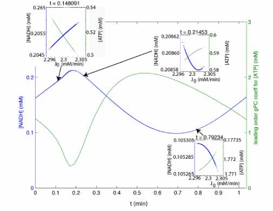
Figure 1: (color online) One period of the oscillation of [NADH] for an ensemble of yeast cells is shown (blue, left axis); one oscillation of the leading order gPC coefficient [ATP] is shown (green, right axis). The relationship of two intracellular concentrations, [NADH] (blue) and [ATP] (green), with respect to the heterogeneity of the glucose influx ($J_{0}$) is shown in the inset figures. Note the continuous dependence of the intracellular concentration on the parameter $J_{0}$.

We have observed in our simulations (and the same phenomenon has been documented in different heterogeneous coupled oscillator contexts (9)) that, after a typical initialization, two distinct phases are observed in the dynamics. During an initial, relatively fast phase, strong correlations develop between the distributions of the various intracellular concentration values; this is followed by a second, long term phase, during which the distributions evolve, but with the correlations “locked in”. In effect, these correlations appear to be strongly related to the heterogeneity of the population - cells with different $J_{0}$ exhibit systematically different concentration patterns. Figure 1 shows the dependence of concentrations of NADH and ATP on the population heterogeneity parameter (the random variable $J_{0}$) at three instantaneous states. There is clearly a relation/dependence between the intracellular metabolite concentrations and the “identity” of the cell (the value of $J_{0}$).

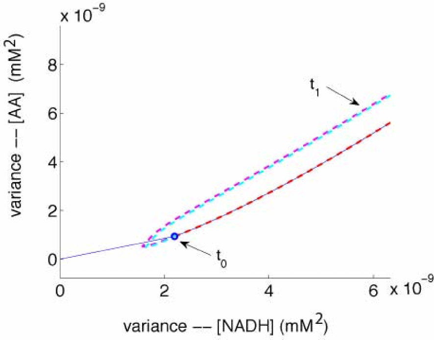
Figure 2: (color online) Phase maps for variances of [NADH] and [AA] in the initial stage. Blue curves: variances computed from realizations located on the fine-level limit cycle. Red curves: variances computed from realizations initialized with the fully correlated lifting from a “blue” coarse initial conditions. The blue circle indicates the location of this initial condition. Magenta and cyan dashed curves: variances computed from realizations initialized with two random liftings from the same coarse initial conditions as above. Note that blue and red curves almost coincide with each other.

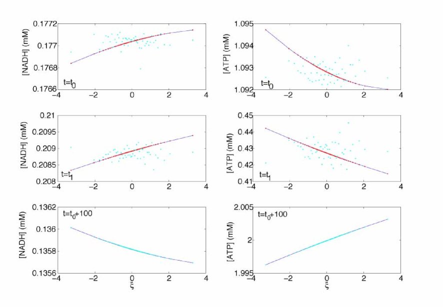
Figure 3: (color online) If the correlations of metabolites within a cell are not incorporated in the lifting (top: cyan dots at time $t_{0}$), then these wrong correlations remain (middle, $t_{1}$) until a sufficiently long amount of time elapses (bottom, $t_{1}+100$). The blue line shows the mature, or natural, correlation. The red dots have been correctly initialized; the cyan points have been initialized with wrong initial correlations. For consistent computations, the relationships between the different metabolites in a cell must be replicated when an ensemble of cells is constructed (in the lifting step).

If the simulation is continued from the exact state where it was interrupted, these correlations remain in place (see the red curves in Figures 2 and 3). If we now create new, artificial initial conditions, where leading moments of the distributions of individual intracellular concentrations are retained but in which the correlations are deliberately scrambled then the system will quickly move away from the synchronized oscillation in a violent transient (see the cyan curves in Figures 2 and 3), and will take a long time to return to it, rebuilding the correlations in the process. These numerical experiments suggest that strong correlations between cell heterogeneity and cell behavior get established during initial stages of the population response, and are then retained in the long term dynamics. Based on this observation, and on the functional dependence of intracellular concentrations on our random variable $\xi$ clearly apparent in Figure 1, we will assume that all intracellular concentrations across the population can, in the long-term dynamics, be expressed as (unknown) functions of the same random variable.

Denoting

$${\bm{x}}(\xi(\omega),t)=(S_{1}(\xi(\omega),t),S_{2}(\xi(\omega),t),S_{3}(\xi(\omega),t),S_{4}(\xi(\omega),t),N_{2}(\xi(\omega),t),A_{3}(\xi(\omega),t))^{T},$$

we will represent ${\bm{x}}$ in terms of a truncated Polynomial Chaos expansion of $\xi$

$${\bm{x}}(\xi,t)=\sum_{j=0}^{P}{\bm{x}}_{c}^{j}(t)\Psi_{j}(\xi).$$ (8)

The fine scale state is the $6001$-long vector of dependent variables (the $6000$ intracellular concentrations plus one extracellular one) in our detailed set of coupled ODEs. Our coarse-grained observables are the gPC truncation coefficients, ${\bm{x}}_{c}^{j}(t)=(x_{1,c}^{j},x_{2,c}^{j},x_{3,c}^{j},x_{4,c}^{j},x_{5,c}^{j},x_{6,c}^{j})^{T}$. The lifting step, the construction of ensemble realizations of intracellular concentrations (fine-level states) consistent with a particular set of values of gPC coefficients (coarse-level observables) is performed through

$${\bm{x}}(\xi_{i},t)=\sum_{j=0}^{P}{\bm{x}}_{c}^{j}(t)\Psi_{j}(\xi_{i}),\quad i=1,2,\cdots,M.$$ (9)

Here $M(=1000)$ is the total number of cells, the truncation level $P$ is set to $3$, and $\{\Psi_{j}\}$ are orthonormal Hermite polynomials (44) for the case of normally distributed $\xi$ . We reiterate that different types of polynomials can be used for random variables obeying different distributions. The total number of our coarse model states is thus $4\times 6+1=25$ (the deterministic extracellular concentration $S_{4,ex}$ is counted here as a single coarse observable); this is clearly much less than the number of internal states, $6M+1$, in the original cell dynamics.

Obtaining the coarse grained observables from a detailed state constitutes the restriction step; our restriction protocol consists of the inner product, Eq. 12, which can be performed in one of two ways: (i) we can discretize the integral to approximate the inner product, i.e., $<{\bm{x}},\Psi_{i}>=1/M\sum_{j=1}^{M}{\bm{x}}(\xi_{j})\Psi_{i}(\xi_{j})$; (ii) we can perform a simple least squares fitting to find ${\bm{x}}_{c}^{j}$ such that an $L^{2}$ norm $||{\bm{x}}(\xi,t)-\sum_{j=0}^{P}{\bm{x}}_{c}^{j}(t)\Psi_{j}(\xi)||$ is minimized. We used the second implementation to obtain gPC coefficients in this work.

In what follows, we will demonstrate two distinct ways of using the EF-UQ methodology in order to accelerate population computations for our model problem. We will first demonstrate direct simulation acceleration through coarse projective integration. We will then demonstrate the accelerated computation and coarse-grained stability analysis of synchronized population oscillations through matrix-free fixed point computation and eigenvalue approximation; these synchronized limit cycles will be computed as fixed points of a coarse Poincaré map. By doing so, we demonstrate that our multiscale toolkit provides a generally applicable and computationally efficient framework for dynamic simulation and analysis of heterogeneous populations of cellular oscillators.

Full direct simulation and coarse projective integration

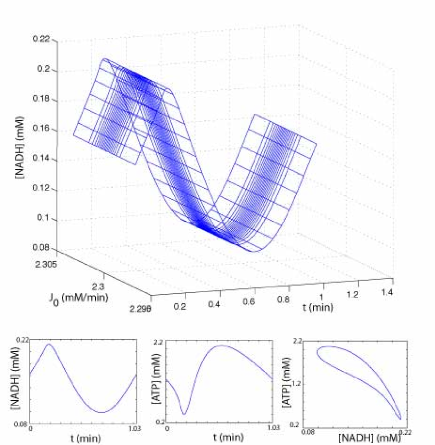
Figure 4: Top: The time series of [NADH] in cells of the ensemble are plotted against time $t$ and the random parameter $J_{0}$ (glucose influx) over one oscillation. The lines transverse to the time series curve are equal-time curves. Bottom left: Time series of the leading order gPC coefficients of [NADH] Bottom right: A projection of the coarse limit cycle onto the leading order [NADH] and [ATP] gPC coefficient plane. The distribution of the glucose influx parameter $J_{0}$ has mean $2.3$ and standard deviation $0.001$.

The full direct simulation consists of integrating of $6M+1$ differential equations ($M$ is the number of cells, 6 internal states for each cell, and 1 extracellular variable). The package ODETools is used in Matlab for this simulation, with variable step-size chosen for relative error tolerance of $1\times 10^{-9}$ and absolute error tolerance of $1\times 10^{-12}$. Figure 4 shows the time history of such a full simulation of an ensemble of cells over one complete period for the distribution of parameter $J_{0}$ having mean $2.3$ and standard deviation $1\times 10^{-3}$. At discrete moments in time, the values of the full ensemble are projected to the gPC basis (the full state is restricted onto coarse observables), also shown in Figure 4. At the fine scale, the concentration of each intracellular metabolite oscillates and, at the end of an oscillation, returns exactly to its starting value. At the coarse, macroscopic level, it is the gPC coefficients that return to themselves. This is, in effect, saying the distributions of the species concentrations return to their initial values.

We now explain the projective integration procedure and compare its results to the direct simulation. Starting at $t=t_{0}$ from a given coarse initial condition (values of the first few gPC coefficients, the observables), we generate fine-level model states by the lifting procedure Eq. 9. We use the original, full dynamic simulation code to evolve the fine-level description for an initial time interval $t_{heal}$; we continue the full direct simulation over three successive time intervals of time $\delta t$. At the end of each of these intervals, the coarse observables are obtained by restriction. The temporal derivatives of the coarse observables can then be estimated (here for convenience we use least squares, but maximum-likelihood based methods are more appropriate (45)); these local time derivatives are then used to project the values of the coarse variables at a time $5\delta t$ further in the future. Using these predicted values we begin the same cycle of brief healing, detailed simulation observed by restriction, estimation of local time derivatives and projection of the coarse behavior into the future. Depending on the coarse projection algorithm used in the forward-in-time projection, more (or fewer) restrictions from the short burst of full simulation may be needed. The particular values of $t_{heal}$ and $\delta t$ can also vary from those used here ($t_{heal}=5\times 10^{-3},\delta t=5\times 10^{-3}$), and their on-line optimal selection is problem-dependent.

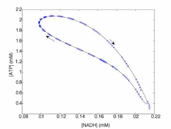
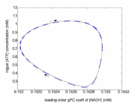
Figure 5: Projective integration in coarse variables (blue) and natural evolution (black). Projective integration accelerates computation of the evolution of a cell population. Top: An ensemble of size $M=1000$ with the distribution of the glucose influx parameter having mean $2.3$ and standard deviation $0.001$. Bottom: An ensemble of $50$ cells, with the distribution of the glucose influx parameters having mean $2.1$ and standard deviation $0.08$. In this regime, there is one free cell, which oscillates at an amplitude relatively larger than the others. For each cell population subplot, the horizontal axis is the leading order gPC coefficient for [NADH]. Top: the vertical axis is the leading order gPC coefficent for [ATP]. Bottom: the vertical axis is [ATP] of the “rogue” cell.

Figure 5 demonstrates the acceleration of the full simulation through a coarse projective forward Euler algorithm. Note that for every $4\delta t$ of full direct simulation, we project $5\delta t$ into the future – only $44.44\%$ of the work is necessary this way. This type of computational savings enables the simulation of larger cell ensembles, allowing more accurate reconstructions of population statistics. As discussed in (46) the method can provide significantly larger savings if a separation of time scales exists in the problem; for linear problems this can be readily seen as a gap between a few leading, slow, and the remaining many, fast eigenvalues of the system. Different coarse projective algorithms (e.g. projective Runge-Kutta, or even implicit projective algorithms) can also be used; linking them to modern estimation techniques and extending them to account for adaptive projective step size selection is the subject of ongoing research (see (47) as well as (48)).

Coarse-grained limit cycle computations

Limit cycle computation. Beyond direct simulation, which asymptotically approaches stable limit cycles, periodic orbits are located by solving boundary value problems in time. In particular, they can be located as fixed points of a Poincaré map (see, for example, the textbook (49)). A Poincaré Section, $S$, is a hypersurface (often a hyperplane) crossing a limit cycle transversely at an (isolated) point. The Poincaré map, $P:S\rightarrow S$, is a return map defined by

$$P({\bm{x}})=\phi_{t}({\bm{x}})\in S,$$

for ${\bm{x}}\in S$, $t$ the smallest positive time for which $\phi_{t}({\bm{x}})\in S$, and $\phi_{t}$ the time $t$ flow map. Note that it is not necessary to know a priori the period of the limit cycle when defining the Poincaré map. Let $P_{f}$ be the Poincaré map for the full simulation and $P_{c}$ be the Poincaré map for the coarse simulation. The two maps are related by

$$P_{c}=R\circ P_{f}\circ L$$

for $R,L$ the restricting and lifting operators and $\circ$ is composition. We use the Newton-Krylov GMRES method to find solutions of $P_{c}({\bm{X}}_{c})={\bm{X}}_{c}$ (50). This implementation of Newton iteration does not explicitly require the computation of the Jacobian of the equation to be solved (often computed in shooting methods through integration of the variational equations). The action of this Jacobian along sequentially selected directions (directional derivatives) is estimated from the results of simulations starting at appropriately chosen nearby initial conditions. Since this only requires simulations of the problem, and the linear equations are solved without ever assembling the relevant Jacobian, this is a matrix-free implementation.

Note that the Poincaré return map can be constructed, not only by direct simulation, but also by projective integration. That is, projective integration can be implemented to accelerate the computations of the Poincaré map itself. The limit cycle in Figure 5 was found by solving this fixed point problem.

Limit cycle stability. For multiscale problems with limit cycles, we can discuss stability at the fine-scale and also at the coarse-grained level. We describe here limit cycle stability computations at both levels, and it is interesting that the results are essentially the same – the coarse-grained stability computations reveal the same information as the (computationally intensive) fine-scale computations.

Let $T$ be the period of the limit cycle, and let ${\bm{x}}_{0}$ be a point on the limit cycle. The time $T$ flow map is $\phi_{T}({\bm{x}}_{0})=x(t;{\bm{x}}_{0})$. Eigenvalues (Floquet multipliers) of the matrix $D\phi_{T}({\bm{x}}_{0})$ (the Jacobian of $\phi_{T}$ at ${\bm{x}}_{0}$, the so-called monodromy matrix) quantify the linearized stability of the limit cycle. The time $T$ coarse flow map is $\Phi_{T}=\Phi_{T}({\bm{X}}_{c})$, see Eq. 18. The matrix $D\Phi_{T}({\bm{X}}_{c})$ can be approximated by finite differences,

$$\left[\frac{\Phi_{T}({\bm{X}}_{c}+\varepsilon e_{1})-{\bm{X}}_{c}}{\varepsilon},\frac{\Phi_{T}({\bm{X}}_{c}+\varepsilon e_{2})-{\bm{X}}_{c}}{\varepsilon},...\right]$$

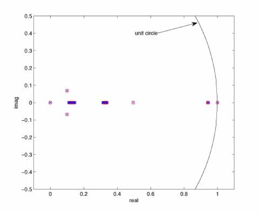
Figure 6: (color online) Leading eigenvalues of $D\phi_{t}^{f}$ (blue, $\times$) and $D\phi_{t}$ (red, $\circ$). The leading eigenvalues are essentially the same, as expected. the unit circle is shown (black curve); note the eigenvalues at 1, and all other eigenvalues are inside the unit circle. analyzing stability of the coarse problem gives insight into the stability of the full cell ensemble.

for $\varepsilon<<1$. The eigenvalues of $D\Phi_{T}({\bm{X}}_{c})$ are shown in Figure 6, and the leading ones are listed in Table 1. Note that the number $1$ is an eigenvalue (corresponding to time translational invariance along the limit cycle at the point $y_{0}$). This invariance gives rise to a neutrally stable direction; all limit cycles possess this neutral eigenvalue at $1$. The magnitudes of the remaining leading eigenvalues of the limit cycle are less than 1 (they lie inside the unit circle). Therefore, the limit cycle is stable.

Eigenvalues of the fine-scale monodromy matrix reveal the stability of the full limit cycle. Divided differences could in principle be used to approximate the full $6001\times 6001$ Jacobian of the fine scale problem; instead, to obtain this matrix we integrated the variational equations (see, for example, the textbook (49)). Let $\dot{\bm{x}}=f({\bm{x}})$; then the variational equations along the solution $x(t,{\bm{x}}_{0})$ are

$$U^{\prime}(t,{\bm{x}}_{0})=Df\left({\bm{x}}(t,{\bm{x}}_{0})\right)\cdot U(t,{\bm{x}}_{0}),$$

where $U(t)$ is a $(6M+1)\times(6M+1)$ matrix and the initial condition $U(0)$ is the identity matrix. This gives

$$D\phi_{T}^{f}({\bm{x}}_{0})=U(T,{\bm{x}}_{0}).$$

The “fine” eigenvalues are shown in Figure 6, and the leading ones are in Table 1.

It can be shown that eigenvalues of the coarse and fine-scale monodromy matrices are theoretically the same (if sufficiently many gPC coefficients are kept), and the coincidence of the eigenvalues is seen in the table. Analysis of the fine-scale model considered here is computationally tractable; for larger problems, however, a full analysis may not be possible, and the coarse stability analysis suffices to characterize stability of the fine-scale limit cycles. For instance, these methods could be profitably applied to large models of coupled biological oscillators involved in yeast respiratory oscillations (51) and mammalian circadian rhythm generation (52).

When coarse-graining fails: “rogue” oscillators

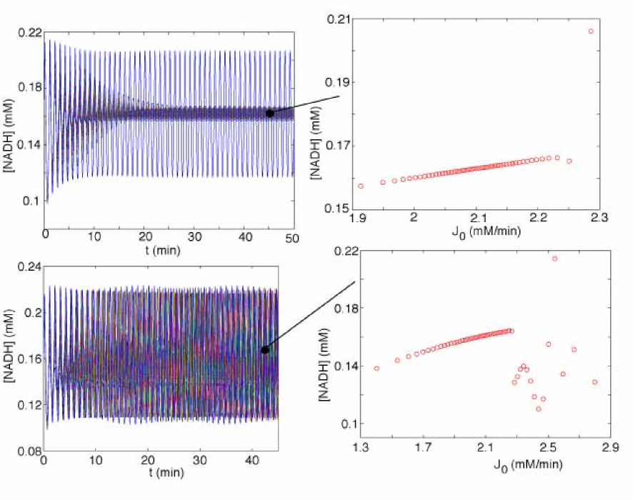
Figure 7: (color online) The discontinuity in the relationship between [NADH] and the parameter $J_{0}$ is shown for distributions with “rogue” oscillators. Top: $J_{0}$ has a Gaussian distribution with mean and standard deviation being 2.1 and 0.08, respectively; bottom: mean $2.1$ and standard deviation $0.3$. The figures on the left show the time history of [NADH] for all 50 cells. The figures on the right show [NADH] as a function of $J_{0}$ at a snapshot in time ($t=45$). Equation-free computations can be applied in these regimes by using more and different coarse variables: gPC coefficients for the “bulk” of the oscillating cells and either gPC coefficients for the other cells or using all the state variables of the other cells.

When the variance of $J_{0}$ is small, NADH concentrations ($N_{2}$) in the cells across the population are narrowly distributed; an overall synchronized solution for the entire population prevails, and our coarse-graining methods are successful. When the variance of $J_{0}$ increases, however, the amplitudes of the $N_{2}$ oscillations across the cell population will separate significantly. For certain combinations of mean and variance of $J_{0}$, one or more cells will appear to oscillate “freely” in amplitude. An illustration of this, using a 50 cell ensemble as the full direct simulation, and setting the mean and standard deviation of $J_{0}$ to 2.1 and 0.08, respectively is seen in Figure 7. The cause of this single “free, oscillating” cell can be clearly rationalized based on the relatively large variance of $J_{0}$: the values of $J_{0}$ across the population spread beyond the parameter point at which the single cell dynamics undergoes a Hopf bifurcation. The strong correlation between individual cell $J_{0}$ values and their detailed states (intracellular concentrations) is retained for most of the cells, but lost for the outlying “rogue” oscillatory cell. As $\sigma_{J}$ continues increasing, the strong correlations that allowed us to use a gPC expansion for the collective behavior fail even more dramatically - see Figure 7, which is quite representative of dynamics in populations with large variance of the glucose influx. We expect that such strong discontinuities in the relation between heterogeneity and detailed state (reminiscent, at some level, of Gibbs phenomena) will, in general, be encountered in probabilistic problems involving strong nonlinearity and bifurcations of the single oscillator behavior as the heterogeneity parameter(s) is varied. Clearly, a few gPC coefficients are no longer good observables of the collective system state. The recent literature includes some efforts in resolving such cases using a wavelet-based chaos expansion (18) or piecewise Polynomial Chaos (17); yet the problem remains an open subject for future research.

Here we will limit ourselves to the case of a single rogue oscillator, shown above. A simple and rational way to tackle this problem is to employ gPC coefficients to describe the oscillators that are “clumped together” with smaller oscillation amplitudes, and use an additional, different set of variables to describe intracellular metabolite concentrations for the single “freely oscillating” cell. More specifically, for a total number $M$ of cells which include one “free” cell, the coarse observables are comprised of $\bm{x}^{0}_{c},\bm{x}^{1}_{c},\cdots,\bm{x}^{P}_{c}$ (obtained by restricting intracellular concentrations of $M-1$ clumped cells through the least-square fitting method mentioned earlier), the extracellular concentration $S_{4,ex}$ and six intracellular concentrations $S_{1},S_{2},S_{3},S_{4},N_{2},A_{3}$ representative of the free cell. When lifting is now implemented, only intracellular concentrations of $M-1$ cells are generated from $\bm{x}^{0}_{c},\bm{x}^{1}_{c},\cdots,\bm{x}^{P}_{c}$ through Eq. 9. The intracellular concentrations $S_{1},S_{2},S_{3},S_{4},N_{2},A_{3}$ for the free cell are part of the coarse-grained description. Therefore, the full direct simulation is again characterized by $6M+1$ variables, but the number of observables of the reduced, coarse-grained problem increases to $4\times 6+1+6=31$ if the first four leading order gPC coefficients are retained ($P=3$).

The initial condition on coarse observables for the projective integration is found by using the equation-free fixed-point algorithm in conjunction with the Poincaré map on the 31-dimensional space. Coarse projective integration for this new, $31$-dimensional coarse grained system is illustrated in Figure 5. Our coarse initial condition is the restriction of a point on the detailed, fine-scale limit cycle solution; starting there, we use short bursts of full direct simulation to estimate the time derivatives of our $31$ coarse observables, and then coarse projective forward Euler to project their values forward in time.

The phase portrait of the coarse-grained limit cycle, projected on the leading order gPC coefficient of the concentration of NADH of the $M-1$ clumped cells and the concentration of ATP in the free cell, is shown in Figure 5. Reasonable numerical agreement with the full direct oscillation (observed on the same variables) prevails; even in the presence of one (more generally, of a few) free cell(s), choosing a good set of coarse-grained variables allows us to accelerate the computations of the long-term system dynamics. Of course, this approach requires a priori identification of the rogue oscillating cells to construct the coarse variables. Clearly more research is needed towards the selection of good coarse observables for such problems.

SUMMARY and CONCLUSIONS

Equation-Free Uncertainty Quantification methods were used in this paper to accelerate the computer-aided analysis of the dynamics of heterogeneous ensembles of coupled biological oscillators; in particular, coarse-grained computations of synchronized population-wide limit cycles and their stability was demonstrated for an ensemble of yeast glycolytic oscillators coupled by membrane exchange of intracellular acetaldehyde. The feasibility of the EF UQ in describing certain particular situations (where one –or a few– oscillator(s) move freely in amplitude, distinguished from the “bulk” of the population) was also demonstrated.

This paper contains only representative “proof of concept” computations. There is a clear necessity for extensive numerical analysis of the schemes illustrated, including adaptive step-size selection, error estimation and control. Different restriction schemes need to be devised when the relation between heterogeneity and behavior becomes nonsmooth or discontinuous in the “randomness direction(s)”. Different lifting schemes (53) exploiting a non-explicit separation of time scales may reduce the number of gPC coefficients required for an accurate reduced description. Furthermore, a wealth of data-mining techniques currently under development (and, in particular, the diffusion map approach (54, 55)) holds the promise of extracting low-dimensional parameterizations of high-dimensional data based on graphs constructed on simulation data and the eigenfunctions of diffusion operators on these graphs. It would be interesting to explore the performance of such techniques when simple gPC observables fail, as in the case of the discontinuities and “multiple oscillator clumps” mentioned above.

APPENDIX A: SOME BASIC UNCERTAINTY QUANTIFICATION (UQ) AND EQUATION FREE UNCERTAINTY QUANTIFICATION (EF-UQ) ISSUES

On polynomial chaos expansion of random variables and processes

Orthogonal polynomials of random variables with an arbitrary probability measure (Gaussian, uniform, Poisson, binomial, …) are called generalized Polynomial Chaos (gPC) (16). Any functional vector, ${\bm{x}}(\omega)$, of random variables, ${\bm{\xi}}(\omega)$ ($=(\xi_{1}(\omega),\cdots,\xi_{n}(\omega))^{T}$), defined over a probability space $(\Omega,{\cal F},P)$, can be expressed in terms of a gPC expansion,

$${\bm{x}}(\omega)=\sum_{i=0}^{\infty}{\bm{x}}_{c}^{i}\Psi_{i}({\bm{\xi}}(\omega)),$$ (10)

where $\Psi_{i}({\bm{\xi}}(\omega))$ is the $i$th generalized Polynomial Chaos which admits the following orthogonality properties,

$$<\Psi_{i},\Psi_{j}>=\left\{\begin{array}[]{ll}<\Psi_{i}^{2}>,&{\rm if\quad i=j},\\ 0,&{\rm if\quad i\neq j},\end{array}\right.$$ (11)

and ${\bm{x}}_{c}^{i}$ is the corresponding coefficient of $\Psi_{i}({\bm{\xi}}(\omega))$, determined by

$${\bm{x}}_{c}^{i}={{<{\bm{x}}(\omega),\Psi_{i}({\bm{\xi}}(\omega))>}\over{<\Psi_{i}^{2}>}}.$$ (12)

In the above equations, the inner product $<\cdot,\cdot>$ is defined by

$$<f({\bm{\xi}}),g({\bm{\xi}})>=\int_{\Gamma}f({\bm{\xi}})g({\bm{\xi}})p({\bm{\xi}})d{\bm{\xi}},\quad{\bm{\xi}}=(\xi_{1}(\omega),\cdots,\xi_{n}(\omega))^{T},$$ (13)

where $p({\bm{\xi}})$ is the joint probability measure of ${\bm{\xi}}$ and $\Gamma$ the support of $p({\bm{\xi}})$.

In the case that ${\bm{x}}$ is a random field or process having the form ${\bm{x}}(\omega,s)$ or ${\bm{x}}(\omega,t)$ where $s$ and $t$ are, respectively, spatial and time coordinates, the projections of ${\bm{x}}$ onto the Polynomial Chaos, ${\bm{x}}_{c}^{i}$, must admit a form that depends on these spatial or time coordinates as well. In our illustrative example the gPC coefficients evolve in (and thus also depend on) time.

On the stochastic Galerkin method

The stochastic Galerkin method aims at quantifying propagation of uncertainty in dynamical systems. In this method, solutions of stochastic systems are first expressed in terms of a finite linear combination of generalized Polynomial Chaos. The error resulting from the finite-term expansion is then required to be orthogonal to test functions, which are normally chosen to be the same as the generalized Polynomial Chaos. A coupled system of equations for the gPC coefficients can thus be derived and solved (12). Probability distributions and statistical moments of the solutions can be computed from the gPC coefficients subsequently.

In particular, let the states of a stochastic system be represented by a vector ${\bm{x}}(\omega,t):\Omega\times\mathbb{R}\rightarrow\mathbb{R}^{N}$, where $\omega$ is an element in the sampling space $\Omega$. This system state is governed by the differential equation

$${{d{\bm{x}}}\over{dt}}={\bm{f}}({\bm{x}},{\bm{\xi}}(\omega)),\quad{\bm{x}}(\omega,0)={\bm{x}}_{0}(\omega).$$ (14)

The solution of the above equation can be approximated by a finite expansion in the form of Eq. 10,

$${\bm{x}}(\omega,t)=\sum_{i=0}^{P}{\bm{x}}_{c}^{i}(t)\Psi_{i}({\bm{\xi}}(\omega)).$$ (15)

By applying a Galerkin projection, equations governing the gPC coefficients ${\bm{x}}_{c}^{i}(t)$ are obtained as

$${{d{\bm{x}}_{c}^{i}}\over{dt}}={1\over{<\Psi_{i}^{2}({\bm{\xi}})>}}<{\bm{f}}(\sum_{i=0}^{P}{\bm{x}}_{c}^{i}(t)\Psi_{i}({\bm{\xi}})),\Psi_{i}({\bm{\xi}})>,\quad i=0,1,\cdots,P,$$ (16)

with ${\bm{x}}_{c}^{i}(0)={{<{\bm{x}}_{0},\Psi_{i}({\bm{\xi}})>}\over{<\Psi_{i}^{2}({\bm{\xi}})>}}$. The above equation can be rewritten as

$${{d{\bm{X}}_{c}}\over{dt}}={\bm{H}}({\bm{X}}_{c}).$$ (17)

Here ${\bm{X}}_{c}=({\bm{x}}_{c}^{0},{\bm{x}}_{c}^{1},\cdots,{\bm{x}}_{c}^{P})^{T}$ and ${\bm{H}}=({\bm{h}}_{0},{\bm{h}}_{1},\cdots,{\bm{h}}_{P})^{T}$, where

$${\bm{h}}_{i}({\bm{X}}_{c})={1\over{<\Psi_{i}^{2}({\bm{\xi}})>}}<{\bm{f}}(\sum_{i=0}^{P}{\bm{x}}_{c}^{i}(t)\Psi_{i}({\bm{\xi}})),\Psi_{i}({\bm{\xi}})>,\quad i=0,1,\cdots,P.$$

If ${{d{\bm{X}}_{c}}\over{dt}}={\bm{0}}$ in the long-time limit, then Eq. 17 has a steady state, which can then be used to recover the probability distribution of the random steady state of Eq. 14. The stochastic Galerkin method can provide an effective reduction of a stochastic model if a relatively small truncation in Eq. 15 above is sufficiently accurate. The corresponding deterministic model will then be considerably easier to simulate and analyze than large numbers of realizations in a Monte Carlo simulation of the original dynamics.

On Equation-Free methods and their application in uncertainty quantification

The basic building block of equation-free methods (20, 21, 22) is the coarse time-stepper, which consists essentially of three components: lifting, micro-simulation, and restriction. Lifting is a procedure to transform a coarse-level state to its fine-level counterpart and restriction the converse of lifting. By employing the model states ${\bm{x}}(t)$ in Eq. 14 as the fine-level system state vector, and their low-order gPC coefficients ${\bm{X}}_{c}$ as the coarse-level observables, Equation-Free methods can be used to numerically study the behavior of gPC coefficients without needing closed form ODEs for their evolution, Eq. 17 (23). The lifting and restriction protocols in our context are then Eq. 15 and Eq. 12, respectively. The micro-simulation is just the simulation of the original large coupled ODE system Eq. 14. Assuming that the long-term coarse-grained dynamics in gPC space lie on a low-dimensional, attracting slow manifold, one can use coarse projective integration to accelerate the computation of successive coarse-level system states, i.e., low-order gPC coefficients ${\bm{x}}_{c}^{i}(t_{j}),i=0,1,\cdots,P,j=0,1,\cdots,M$, through restriction of (one or more) short bursts of fine scale simulation as follows: Temporal derivatives ${d{\bm{x}}_{c}^{i}}\over{dt}$ at $t_{M}$ are estimated by least-squares fitting of the short-time gPC coefficient evolution ${\bm{x}}_{c}^{i}(t_{j}),j=M-k,M-k+1,\cdots,M,k<M$. These gPC coefficients in conjunction with their locally estimated temporal derivatives are then used to extrapolate (in effect, integrate the gPC coefficients numerically in time) over a relatively large coarse time interval $T$. For instance, if the coarse forward Euler projective integration is used, then the predicted gPC coefficients at a later time $t_{M}+T$ are obtained by

$${\bm{x}}_{c}^{i}(t_{M}+T)\approx{\bm{x}}_{c}^{i}(t_{M})+{{d{\bm{x}}_{c}^{i}}\over{dt}}(t_{M})T,\quad i=0,1,\cdots,P.$$

These projected in time gPC coefficients ${\bm{x}}_{c}^{i}(t_{M}+T)$ are lifted again to the full fine state level, and a new short burst of micro-simulation is initiated. The procedure is repeated until a desired time limit is reached. Issues of time-step selection, estimation and error control are important, and often “the devil lies in these details”; discussing these numerical analysis issues, however, is not the aim of this brief exposition, and we refer the reader to (46, 47, 56, 21).

If equation Eq. 17 possesses a steady state ${\bm{X}}_{c}^{s}$, then ${\bm{X}}_{c}^{s}$ must satisfy an integral form of Eq. 17 given by

$${\bm{X}}_{c}^{s}={\bm{X}}_{c}^{s}+\int_{t_{0}}^{t_{0}+T}{\bm{H}}({\bm{X}}_{c})dt$$ (18)

where ${\bm{X}}_{c}(t_{0})={\bm{X}}_{c}^{s}$. The right-hand side of Eq. 18 can be viewed as a time flow $\Phi_{T}:\mathbb{R}^{N\times(1+P)}\times\mathbb{R}\rightarrow\mathbb{R}^{N\times(1+P)}$. Therefore, the steady state ${\bm{X}}_{c}^{s}$ is the fixed-point of the equation

$${\bm{X}}_{c}=\Phi_{T}({\bm{X}}_{c}).$$ (19)

When the above equation is not explicitly available, we can use the coarse time-stepper to approximate the time flow $\Phi_{T}$. Newton’s method or other iterative algorithms, often in matrix-free implementations, can be readily employed to compute steady-state gPC coefficients, which can be used to reconstruct random stable/unstable steady states of the original system, Eq. 14. It is also possible to compute limit cycles of the gPC coefficients through Poincaré return maps, thus linking EF methods with the analysis on random limit cycles.

ACKNOWLEDGEMENTS This work was partially supported by DARPA, and by an NSF Graduate Research Fellowship to K.B.

Leading eigenvalues
coarse eigenvalues	full eigenvalues
1.000004	1.000219
0.942622	0.9426798
0.496275	0.4962654
0.328651	0.3273728
$0.100267\pm 0.068410i$	$0.100250\pm 0.0683621i$
0.126292	0.126075

Table 1: Selected, leading eigenvalues from the computations of the coarse level and of the fine level are shown. The eigenvalue at 1 corresponds to a neutrally stable direction along the limit cycle.

References

- Winfree (2001) Winfree, A. T. 2001. The geometry of biological time. volume 12 of Interdisciplinary Applied Mathematics. Springer-Verlag, New York. second edition.
- Goldbeter (1996) Goldbeter, A. 1996. Biochemical Oscillations and Cellular Rhythms: The Molecular Bases of Periodic and Chaotic Behaviour. Cambridge University Press, Cambridge, UK.
- Strogatz (2003) Strogatz, S. H. 2003. Sync: The Emerging Science of Spontaneous Order. Hyperion, New York, NY.
- Acebrón et al. (2005) Acebrón, J. A., L. L. Bonilla, C. J. Pérez Vicente, F. Ritort, and R. Spigler. 2005. The kuramoto model: A simple paradigm for synchronization phenomena. Rev. Mod. Phys. 77:137–185.
- Strogatz (2000) Strogatz, S. H. 2000. From Kuramoto to Crawford: exploring the onset of synchronization in populations of coupled oscillators. Physica D 143:1–20. Bifurcations, patterns and symmetry.
- Forger and Peskin (2003) Forger, D. B., and C. S. Peskin. 2003. A detailed predictive model of the mammalian circadian clock. PNAS 100:14806–14811.
- Michel and Colwell (2001) Michel, S., and C. S. Colwell. 2001. Cellular communication and coupling within the suprachiasmatic nucleus. Chronobiol. Int. 18:579–600.
- Moon and Kevrekidis (2006) Moon, S. J., and I. G. Kevrekidis. 2006. An equation-free approach to coupled oscillator dynamics: the kuramoto model example. International Journal of Bifurcations and Chaos 16:2043–2052.
- Moon et al. (2006) Moon, S. J., R. Ghanem, and I. G. Kevrekidis. 2006. Coarse-graining the dynamics of coupled oscillators. Phys. Rev. Lett. 96.
- Fishman (1996) Fishman, G. 1996. Monte Carlo: concepts, algorithms, and applications. Springer-Verlag, New York.
- Schuler and Domach (1983) Schuler, M. L., and M. Domach. 1983. Mathematical models of the growth of individual cells. In Foundations of Biochemical Engineering, American Chemical Society 93–133.
- Ghanem and Spanos (1991) Ghanem, R. G., and P. D. Spanos. 1991. Stochastic Finite Elements: A Spectral Approach. Springer-Verlag, New York.
- Ghanem (1998) Ghanem, R. 1998. Probabilistic characterization of transport in heterogeneous porous media. Computer Methods in Applied Mechanics and Engineering 158:3–4.
- Maitre et al. (2001) Maitre, O. L., O. Knio, M. Reagan, H. Najm, and R. Ghanem. 2001. A stochastic projection method for fluid flow. i: Basic formulation. J. Comp. Phys. 173:481–511.
- Reagan et al. (2004) Reagan, M., H. Najm, B. Debusschere, O. L. Maitre, O. Knio, and R. Ghanem. 2004. Spectral stochastic uncertainty quantification in chemical systems. Combustion Theory and Modelling 8:607–632.
- Xiu and Karniadakis (2002) Xiu, D. B., and G. E. Karniadakis. 2002. The wiener-askey polynomial chaos for stochastic differential equations. SIAM J. Sci. Comput. 24:619–644.
- Deb et al. (2001) Deb, M. K., I. M. Babuška, and J. T. Oden. 2001. Solution of stochastic partial differential equations using Galerkin finite element techniques. Comput. Methods Appl. Mech. Engrg. 190:6359–6372.
- Maitre et al. (2004) Maitre, O. L., O. Knio, H. Najm, and R. Ghanem. 2004. Uncertainty propagation using Wiener-Haar expansions. J. Comp. Phys. 197:28–57.
- Reagan et al. (2003) Reagan, M., H. Najm, O. Knio, R. Ghanem, and O. Lemaitre. 2003. Uncertainty propagation in reacting-flow simulations through spectral analysis. Combustion and Flame 132:545–555.
- Theodoropoulos et al. (2000) Theodoropoulos, C., Y.-H. Qian, and I. G. Kevrekidis. 2000. Coarse stability and bifurcation analysis using time-steppers: A reaction-diffusion example. PNAS 97:9840–9843.
- Kevrekidis et al. (2003) Kevrekidis, I. G., C. W. Gear, J. M. Hyman, P. G. Kevrekidis, O. Runborg, and C. Theodoropoulos. 2003. Equation-free, coarse-grained multiscale computation: enabling microscopic simulators to perform system-level analysis. Commun. Math. Sci. 1:715–762.
- Kevrekidis et al. (2004) Kevrekidis, I. G., C. W. Gear, and G. Hummer. 2004. Equation-free: the computer-assisted analysis of complex, multiscale systems. AIChE J. 50:1346–1354.
- Xiu et al. (2005) Xiu, D. B., R. Ghanem, and I. G. Kevrekidis. 2005. An equation-free approach to uncertain quantification in dynamical systems. IEEE Computing in Science and Engineering Journal (CiSE) 7:16–23.
- Henson et al. (2002) Henson, M. A., D. Muller, and M. Reuss. 2002. Cell population modeling of yeast glycolytic oscillations. Biochem. J. 368:433–446.
- Wolf and Heinrich (2000) Wolf, J., and R. Heinrich. 2000. Effect of cellular interaction on glycolytic oscillations in yeast: A theoretical investigation. Biochem. J. 345:321–334.
- Aon et al. (1992) Aon, M. A., S. Cortassa, H. V. Westerhoff, and K. van Dam. 1992. Synchrony and mutual stimulation of yeast cells during fast glycolytic oscillations. J. General Microbiology 138:2219–2227.
- Dano et al. (1999) Dano, S., P. G. Sorensen, and F. Hynne. 1999. Sustained oscillations in living cells. Nature 402:320–322.
- Das and Busse (1991) Das, J., and H. G. Busse. 1991. Analysis of the dynamics of relaxation type oscillation in glycolysis of yeast extracts. Biophys. J. 60:363–379.
- Betz and Chance (1965) Betz, A., and B. Chance. 1965. Phase relationship of glycolytic intermediates in yeast cells with oscillatory metabolic control. Archives of Biochemistry and Biophysics 109:585–594.
- Das and Busse (1985) Das, J., and H.-G. Busse. 1985. Long term oscillations in glycolysis. J. Biochem. 97:719–727.
- Kreuzberg and Martin (1984) Kreuzberg, K., and W. Martin. 1984. Oscillatory starch degradation and fermentation in the green algae chlamydomonas reinhardii. Biochem. Biophys. Acta. 799:291–297.
- Tornheim (1988) Tornheim, K. 1988. Fructose 2,6-bisphosphate and glycolytic oscillations in skeletal muscle extracts. J. Biol. Chem. 263:2619–2624.
- Chance et al. (1965) Chance, B., J. R. Williamson, D. Jamieson, and B. Schoener. 1965. Properties and kinetics of reduced pyridine nucleotide fluorescence of the isolated and in vivo rat heart. Biochem. J. 341:357–377.
- Ibsen and Schiller (1967) Ibsen, K. H., and K. W. Schiller. 1967. Oscillations of nucleotides and glycolytic intermediates in aerobic suspensions of Ehrlich ascites tumor cells. Biochem. Biophys. Acta. 799:291–297.
- Ghosh et al. (1971) Ghosh, A. K., B. Chance, and E. K. Pye. 1971. Metabolic coupling and synchronization of NADH oscillations in yeast cell populations. Archives of Biochemistry and Biophysics 145:319–331.
- Richard et al. (1996) Richard, P., B. M. Bakker, B. Teusink, K. van Dam, and H. V. Westerhoff. 1996. Acetaldehyde mediates the synchronization of sustained glycolytic oscillations in populations of yeast cells. Eur. J. Biochem. 235:238–241.
- Richard et al. (1994) Richard, P., J. A. Diderich, B. M. Bakker, B. Teusink, K. van Dam, and H. V. Westerhoff. 1994. Yeast cells with a specific cellular make-up and an environment that removes acetaldehyde are prone to sustained glycolytic oscillations. FEBS Letters 341:223–226.
- Bier et al. (2000) Bier, M., B. M. Bakker, and H. V. Westerhoff. 2000. How yeast cells synchronize their glycolytic oscillations: A perturbation analytic treatment. Biophys. J. 78:1087–1093.
- Goldbeter and Lefever (1972) Goldbeter, A., and R. Lefever. 1972. Dissipative structures for an allosteric model. Application to glycolytic oscillations. Biophys. J. 12:1302–1315.
- Selkov (1975) Selkov, E. E. 1975. Stabilization of energy charge, generation of oscillation and multiple steady states in energy metabolism as a result of purely stoichiometric regulation. Eur. J. Biochem. 59:151–157.
- Wolf and Heinrich (1997) Wolf, J., and R. Heinrich. 1997. Dynamics of two-component biochemical systems in interacting cells: Synchronization and desynchronization of oscillations and multiple steady states. Biosystems 43:1–24.
- Hynne et al. (2001) Hynne, F., S. Dano, and P. Sorensen. 2001. Full-scale model of glycolysis in . Biophys. Chem 94:121–163.
- Wolf et al. (2000) Wolf, J., J. Passarge, O. J. G. Somsen, J. L. Snoep, R. Heinrich, and H. L. Westerhoff. 2000. Transduction of intracellular and intercellular dynamics in yeast glycolytic oscillations. Biophys. J. 78:1145–1153.
- Abramowitz and Stegun (1970) Abramowitz, M., and I. Stegun. 1970. Handbook of Mathematical Functions. Dover Publications, Inc., New York.
- Aït-Sahalia (2002) Aït-Sahalia, Y. 2002. Maximum likelihood estimation of discretely sampled diffusions: a closed-form approximation approach. Econometrica 70:223–262.
- Gear and Kevrekidis (2002) Gear, C. W., and I. G. Kevrekidis. 2002. Projective methods for stiff differential equations: Problems with gaps in their eigenvalue spectrum. SIAM Journal of Scientific Computing 24:1091–1106.
- Gear and Kevrekidis (2003) Gear, C. W., and I. G. Kevrekidis. 2003. Telescopic projective methods for parabolic differential equations. J. Comput. Phys. 187:95–109.
- Lee and Gear (2005) Lee, S. L., and C. W. Gear. 2005. Second-order accurate projective integrators for multiscale problems. UCRL-JRNL-212640 .
- Hirsch et al. (2004) Hirsch, M. W., S. Smale, and R. L. Devaney. 2004. Differential equations, dynamical systems, and an introduction to chaos. volume 60 of Pure and Applied Mathematics (Amsterdam). Elsevier/Academic Press, Amsterdam. second edition.
- Kelley (1995) Kelley, C. T. 1995. Iterative Methods for Linear and Nonlinear Equations. SIAM.
- Henson (2004) Henson, M. A. 2004. Modeling the synchronization of yeast respiratory oscillations. Journal of Theoretical Biology 231:443–458.
- To et al. (accepted for publication) To, T.-L., M. A. Henson, E. D. Herzog, and F. J. Doyle III. accepted for publication. A computational model for intercellular synchronization in the mammalian circadian clock. Biophys. J. .
- Gear et al. (2005) Gear, C. W., T. J. Kaper, I. G. Kevrekidis, and A. Zagaris. 2005. Projecting to a slow manifold: singularly perturbed systems and legacy codes. SIAM J. Appl. Dyn. Syst. 4:711–732 (electronic).
- Belkin and Niyogi (2003) Belkin, M., and P. Niyogi. 2003. Laplacian eigenmaps for dimensionality reduction and data representation. Neural Computation 15:1373–1396.
- Nadler et al. (2006) Nadler, B., S. Lafon, R. R. Coifman, and I. G. Kevrekidis. 2006. Difusion maps, spectral clustering and reaction coordinates of dynamical systems. Appl. Comput. Harmon. Anal. 21:113–127.
- Gear et al. (2002) Gear, C. W., I. G. Kevrekidis, and C. Theodoropoulos. 2002. Coarse integration/bifurcation analysis via microscopic simulators: Micro-Galerkin methods. Computers and Chemical Engineering 26:941–963.